Abstract
The International Maritime Organization (IMO) Decarbonization Roadmap for curbing and eliminating Greenhouse Gas (GHG) emissions by 2030 and 2050, respectively, is a “herculean” task in its own respect. If it is now combined with fundamental changes in trade dynamics, volatile market conditions, tighter shipping financing platforms with sustainability-linked interest rates and international safety regulations setup, a completely new framework for commercial ship design characterized by strict and often contradicting requirements emerge In parallel, zero carbon fuels available (readily or in the future) require extensive technological modifications and technical leaps in the current arrangements ship propulsion plants (with little to no existing reference) characterized by elevated consumption figures due to low energy density leading to an overshoot in voyage expense costs and the Total Cost of Ownership (TCO), respectively. Considering such a tight design space, holistic approaches with lifecycle considerations aiming at robust designs are deemed necessary. Pursuant to this roadmap, the authors have developed a design methodology fully integrated within the CAE software CAESES™ that encompass all aspects of ship design (stability, strength, powering and propulsion, safety, economics) and has an inherent dynamic voyage simulation module, enabling the user to simulate the response in variations of the geometrical, design variables of the vessel under uncertainty. The methodology has been extended to model the design and propulsion plant of an Ammonia powered Large Bulk carrier and deployed in global ship design optimization studies and utility-based ranking and selection process.
1. Introduction
The International Maritime Organization (IMO), which is the primary international and inter-governmental regulatory for maritime matters, has developed several regulations in the past two decades focusing on marine safety (through its Marine Safety Committee—MSC) as well as protection of the marine environment (through its Marine Environmental Protection Committee—MEPC). In April 2018 and during the session of MEPC72 (followed by the session of MEPC73), the International Maritime Organization pledged a 50% reduction of the shipping-generated GHGs by year 2050 when compared to the emission levels of 2008, with the intention to reduce more than 70% by the end of the century [1]. In the meantime, the global trade relations that evolved from the first and second decade of the 21st century have resulted in alternating periods of growth and economic recession triggering an unprecedented volatility in shipping freight rates (due to supply/demand imbalance), posing considerable threats to the fiscal and commercial sustainability of numerous shipping companies. Such an ambitious decarbonization roadmap coupled with multiple threats and challenges in the economic sector require the re-evaluation of not only the current design templates for major commercial vessels but also the entire Preliminary and Basic Ship Design Process. It is the authors’ belief that this process should be shifted and evolved to simulation-based methods that integrate advanced prediction analytical tools as well as numerical methods from the early stages of the ship design spiral [2], especially when weighing in the increasing costs of net zero carbon fuels [3], as well the equipment and machinery costs for handling such fuels and their impact on both the CAPEX and OPEX. Among the different net zero carbon fuels currently studied in the industry is ammonia (NH3). On the one hand, the latter has low energy density (due to its low calorific value) [4], which corresponds to a threefold increase in fuel consumption with subsequent effects on the increased capacity requirements for the cryogenic storage of ammonia. On the other hand, the complete absence of carbon from its molecule corresponds to a drastic decrease in shipborne CO2 emissions without the need of exhaust aftertreatment (e.g., carbon capturing), equivalency measures (biofuels being carbon zero on a net basis) or expensive production techniques (electro-fuels). Combined with a potential for industrial scalability, ammonia is a strong candidate for large, ocean-going vessels such as tankers and bulk carriers with some preliminary design concept renderings. However, in order for such concepts to be commercially viable, a simulation-driven optimization approach instead of the traditional single-point hull optimization approaches is necessary.
In the context of the above challenges and tasks, the present paper focuses on presenting the application of a Robust Holistic Optimization Design Approach (RHODA) which is applied on the optimization of the design of ammonia-powered, zero-emission Capesize bulk carriers and Very Large Ore Carriers (VLOC) through systematic optimization utilizing a power computational framework and design methodology. The already proven RHODA method that is holistic, robust through extensive modelling of multiple layers of uncertainty and based on voyage simulation is deployed for the basic ship design of zero emission bulk carriers. The voyage simulation module aims at simulating the vessel’s operation over its entire lifecycle and under real voyage conditions with the addition of advanced uncertainty of environmental and market conditions, focusing on the minimization of all operating costs and maximization of income, as best expressed by the Required Freight Rate (RFR) on the one hand and the minimization of the energy footprint of the vessel and associated CO2-equivalent lifecycle emissions on the other. New metrics are also introduced in the form of the Maximum Ammonia Price (MAP) index and Required Carbon Tax (RCT) to provide regulatory and market guidance on the sustainable levels of zero emission fuel pricing.
The paper’s structure contains four sections. In Section 2, the Robust Holistic Optimization Design Approach (RHODA) is briefly described along with the adaptations required for modeling Zero Emission Vessels. In Section 3, the systematic global optimization studies for zero emission bulk carriers (of large size) are presented along with the results, dominant variants and post-processing studies followed by a comprehensive discussion of findings in Section 4, which features, apart from a systematic dissemination of the results, a projection and a more generic discussion on the design, economic and environmental performance of ZEVs and offers the “lessons learned” for future design studies.
2. Robust Holistic Optimization Design Approach (RHODA)
The effects of uncertainty during all stages of ship design as well as its implications in optimization studies is an already well-studied topic in the literature with notable examples, such as works [5,6] examining two methods of uncertainty modeling for ship design optimization, those of robust optimization and reliability-based optimization. An example of a reliability-based design use of uncertainties in a ship design multi-disciplinary optimization model is presented in [7]. A two-stage stochastic programming for robust ship design optimization under uncertainty was developed in [8,9]. A stochastic design methodology to account for uncertainties in the early ship design process was examined by Plessas and Papanikolaou [10]. This study was subsequently expanded by Plessas et al. [11]. The weather uncertainties of the route, including sea currents, are not considered, nor is any variation introduced in local hull form characteristics and cargo tank arrangement parameters. Furthermore, the methodology focuses on solving a predefined route with a “static approach” to the self-propulsion equilibrium, not considering the engine loading limitations (torque limiters) and specific responses. The embedding of a vessel’s operation simulation within the early design process has not been adequately studied in the literature, with only a handful of relevant examples available. Within the topic of simulation in early ship design, Tillig et al. [12,13] proposed a generic ship energy systems model that can predict the ship’s energy consumption during different operational conditions, without, however, taking into account variation in the vessel’s RPM, heavy running and potential limitations from the engine’s torque (fuel) limit. In [14], an event-based simulation model was utilized in order to reduce the simulation cost using an event-based operational profile instead of a time-domain simulation of vessel operation, using discrete event simulation for analyzing system performance. A quasi-static discrete-event simulation model to replicate and assess the voyage of a general cargo vessel was proposed in [15]; a prescribed route was used based on real-time (15 min) data and a constant speed assumption; it could be potentially integrated in a design environment. However, such approaches are “decoupled” from the propeller and main engine. More specifically, the actual operating point of the propeller and shift of self-propulsion equilibrium and advance coefficient are not considered in applications that try to introduce voyage simulation in ship design optimization. Furthermore, the codes are static and do not follow an approach of voyage legs and dynamic conditions but instead use a more static calculation. In view of this, the authors introduce a new method called Robust Holistic Optimization Design Approach (RHODA).
The method belongs in the holistic ship design approaches. The term holism originates from the Greek word ὅλος (meaning all, entire, total). This philosophical notion asserts that all the properties of a given system (biological, chemical, social, economic, mental, linguistic, etc.) cannot be determined or explained by the sum of its component parts alone. Instead, the system as a “whole” determines an important way in which the parts behave. Aristotle in Metaphysics (H-6, 1045a8–10) [16] examines the problem of the unity of definition and offers a new solution based on the concepts of potentiality and actuality. Holistic ship design approaches have been introduced in [17,18,19], where the generic ship design optimization problem is defined and presented in its holistic nature. The typical process flow of computational methodologies for performing all the necessary computations included in the different design aspects is also defined within the same context of the holistic ship design theory [20,21] aimed at the systematic, risk-based optimization of AFRAMAX tankers, focusing on the cargo carrying capacity, steel weight and accidental oil outflow.
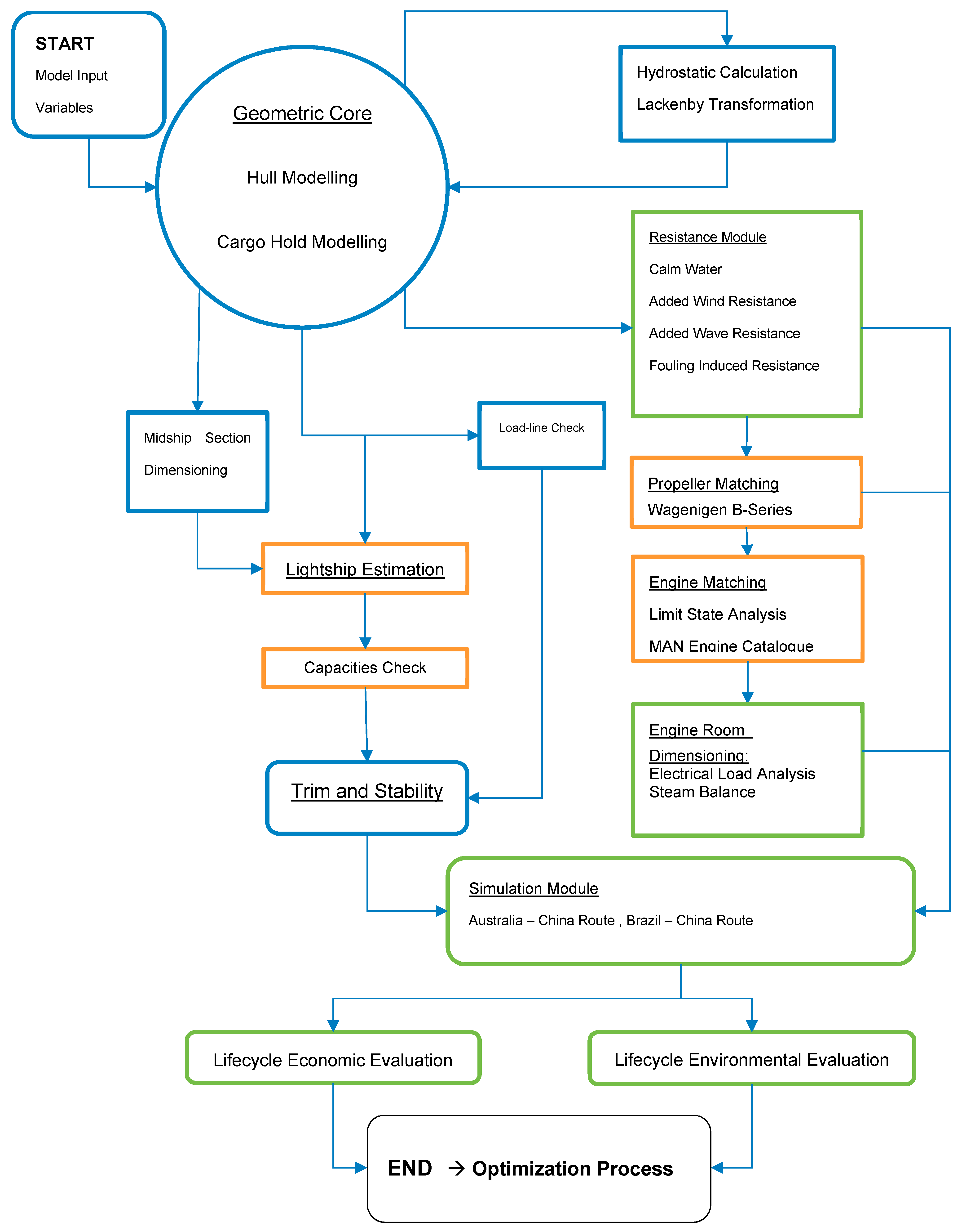
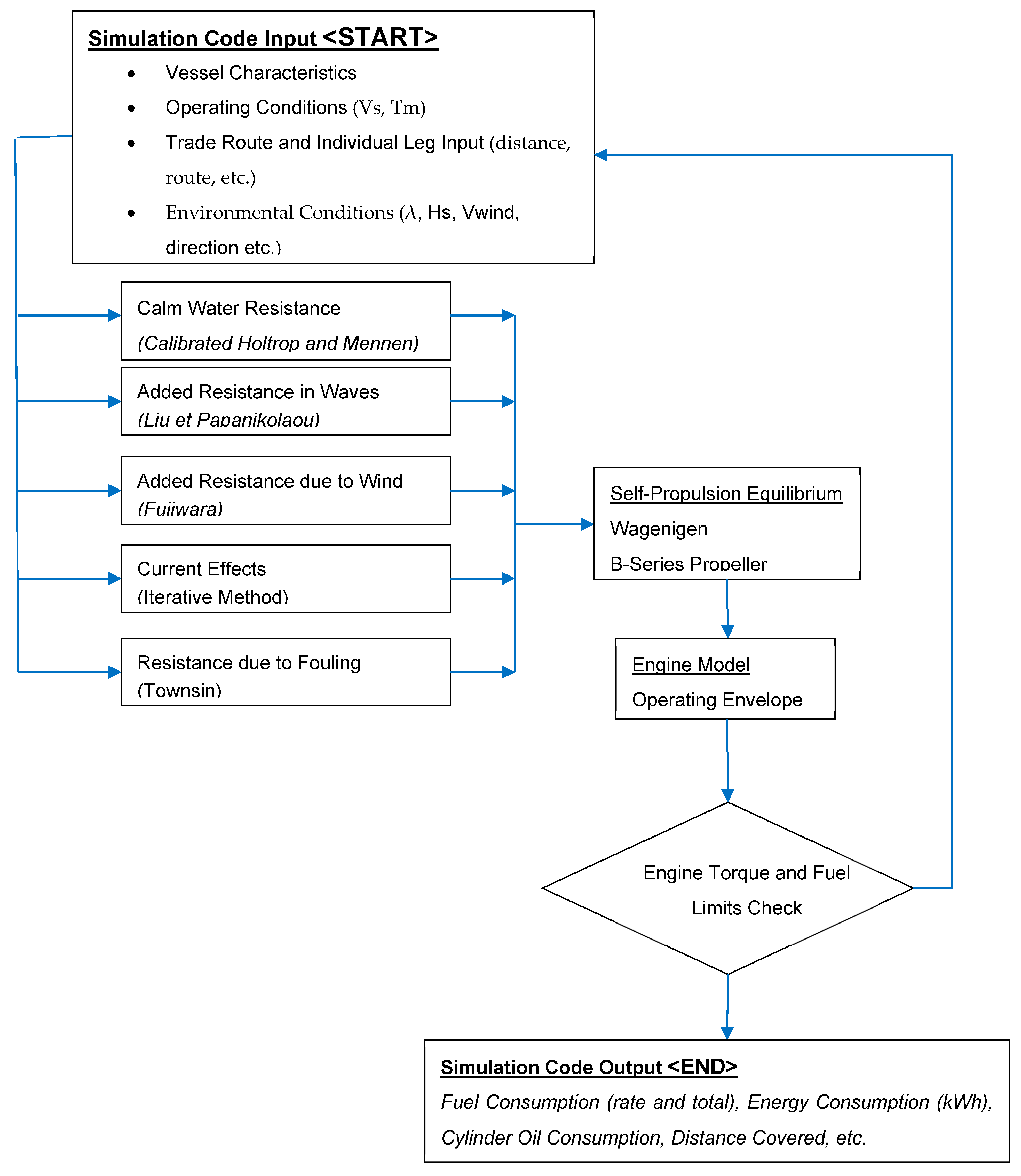
Using the above work and the previous work of the authors and development of such design methodologies within the ship design laboratory of the National Technical University of Athens, the authors herein present an evolved and further enhanced method fully incorporated in the CAESES® CAD/CAE environment. The methodology is holistic, in the sense that all of the critical aspects of the design are addressed under a common framework that takes into account the lifecycle performance of the ship in terms of safety efficiency and economic performance, the internal system interactions as well as the parameter correlations, design trade-offs and sensitivities. The workflow of the methodology has the same tasks as the traditional design spiral; the difference is that the approach is not sequential but concurrent. The primary novelty of the herein presented methodology is that it is simulation-driven in the sense that the assessment of the key design attributes for each variant is derived after the simulation of the vessel’s operation under different voyage profiles for its entire lifecycle instead of using a prescribed loading condition and operating speed [22,23]. The environment in which the methodology is programmed and is responsible for the generation of the fully parametric hull surfaces is the CAESES CAE. The proposed RHODA methodology has the workflow depicted in Figure 1, with the RHODA process taxonomy described in Table 1.
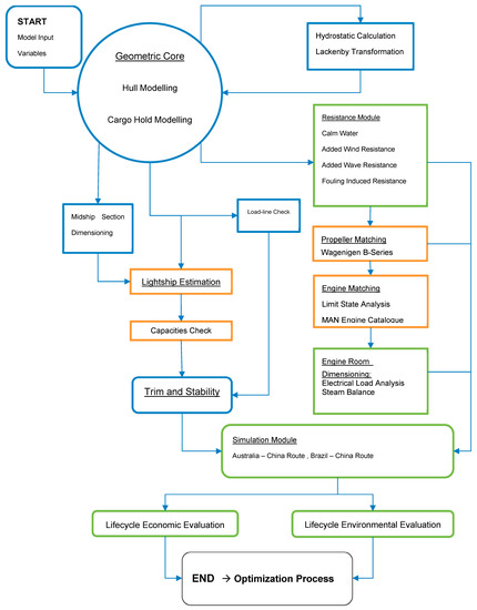
Figure 1.
Overview of the Robust Holistic Optimization Design Approach (RHODA) the study is based on.

Table 1.
List of RHODA Processes and Taxonomy.
2.1. Voyage Simulation Module
One of the novel aspects of the deployed RHODA methodology is the voyage simulation module applicable for each design variant based on big data and the statistical analysis of the latter with the IBM SPSS® (v. 23) toolkit and various statistical and mathematical models embedded. The “big data” in question are key parameters and onboard data collected from an automated high-frequency data acquisition system, Vessel Performance Monitoring System (VPMS). The latter collects and logs real-time data recorded on a 30 s basis. The 30 s recording entries are automatically averaged into 5 min bundles that are accessible and transmitted three times per day ashore. The big data captured onboard are used for the following functions:
- Creation of voyage profile that is input in simulation module.
- Creation of Probability Distribution Functions (PDF) for environmental conditions (Wind, Wind Direction, Wave, Wave Direction, Current and Current Direction, etc.) with either data captured onboard or coordinate-matched satellite hindcast.
- Creation of PDFs for operating speed per voyage profile leg.
For each one of the voyage legs (given distance in nautical miles), the vessel’s particulars, ordered leg speed and calm water resistance curves are input, as well as the loading of the generators and the maneuvering time. If the leg includes a discharging, loading or bunkering port, the port stay in hours is also used. Based on this profile, the voyage-associated costs, together with the fuel costs, are calculated on a much more accurate and realistic basis. Each voyage is broken into distinct geographical legs for which a separate voyage profile is modelled and adjusted. The operating speed is calculated using the average leg speed and determining the probability of a +/−20% deviation resulting in a probabilistic ordered speed (speed over ground/SoG). As the input for each resistance calculation module is Speed Through Water (StW), the current calculation model is in turn activated. Current effects are captured using the iterative method of ISO 15016-2016 [24] on the ordered, SoG value. The correction to the operating speed is positive for the cases of astern current and negative for the cases of ahead current. All currents are considered for arbitrary directions, both in the ahead and astern term and trigonometrically split in an active current (longitudinal axis) and drift current (transverse axis) that only yields deviation rather than speed loss. The final resulting StW with current effects is then used as input in the next simulation sub-routines. From the above-mentioned two corrections, the probabilistic ship speed is derived and based on this the calm water resistance, delivered power and added resistance and power calculations take place. First, the Calm Water Resistance for the corrected Ordered Speed is calculated from Calm Water Resistance-developed curves (for ballast and laden conditions) in the corresponding module of the RHODA. The added resistance module is called from within the operational simulation module on a user-defined time-step (continuous model) with the final estimation calculated on a probabilistic and spectral basis for different wave directions, wave heights and wave lengths, resulting in a single figure for a developed seaway determined from the environmental model deployed. Depending on the months since the last dry dock (input variable), the increase in hull roughness and corresponding hull frictional resistance is calculated using the sub-routines of the corresponding RHODA module. After this assessment, a total resistance module for each time step in each voyage leg is calculated. For this given speed resistance value (kN) and considering the chosen (optimized) propeller characteristic curves (Kt, Kq), the propeller operating point per time stamp and leg is derived. A parallel check is also run with regard to the derived operating point of the propeller and its relevant position in the engine envelope in order to ensure that the (RPM, Power) point does not exceed the torque limits of the engine. In such a case, the RPMs are controlled with the same PI controller philosophy as in a modern two-stroke marine diesel engine governor with involuntary loss of speed as a result. The final determination of the operating point of the hull–propeller–main engine results in the final value of delivered power, as well as the resulting consumption and efficiency figures which are summed for the entire voyage as well as on annual and lifecycle bases. The above are summarized in Figure 2 below.
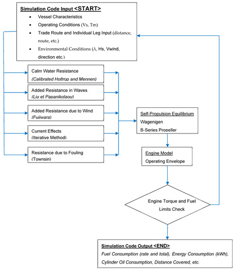
Figure 2.
Voyage Simulation Module Process Flow in RHODA.
2.2. Lifecycle Economic Evaluation
For the proposed lifecycle economic assessment, first, the charter market of large bulk carriers is modelled based on historical data for the Time Charter Equivalent (TCE), acquisition and disposal (scrapping/recycling) prices from 1990 to 2015 as extracted from Clarkson’s Shipping Intelligence database [25]. The following data are extracted and edited for the years 1990 to 2015:
- Capesize 176–180 k DWT Newbuilding prices in millions of USD,
- Capesize Scrap Value in millions of USD,
- Indian Sub-continent Demolition prices in USD/LDT (light weight tons),
- Far East Sub-continent Demolition prices in USD/LDT (light weight tons),
- Capesize Long Run Historical Earnings in USD/day,
- Capesize Fleet Development in number of vessels and deadweight.
In the second stage, the new Newbuilding price ratio (USD/lightship ton) is correlated to the corresponding month’s Capesize Earnings in USD/day [25]. This is performed with the IBM SPSS® Statistical kit after running descriptive statistics and normality checks, resulting in the below non-linear regression expression:
The same approach has been followed for the expression of the Scrap value (disposal value) using the India/Bangladesh Demolition values from 1990 to 2015 from [25]:
As a result of the above correlations, the acquisition and disposal prices can now also have their own corresponding PDFs deriving from the developed PDF for Capesize Earnings depicted in Figure 3 and described in Table 2.
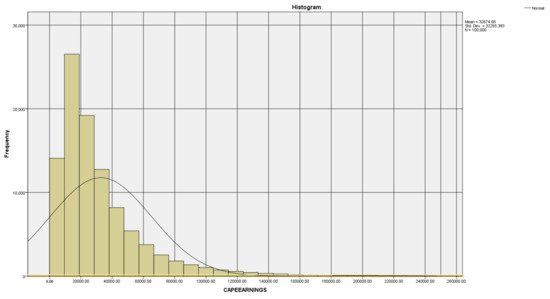
Figure 3.
Histogram of the populated values for Capesize Earnings from 1990 to 2015.
Table 2.
Fitted Probability Distribution Function for TCE Earnings.
All categories in OPEX have been modelled from the reported data of a stock exchange listed bulk carrier ship management company. The Required Freight Rate (RFR) is the most common index used in ship design for assessing the economic performance of a candidate vessel. Assuming that the vessel operates in the spot market, the RFR is expressing the minimum amount of income in USD per ton of cargo transported in order for the vessel to have a breakeven between cash inflows and outflows taking into account the acquisition cost, the disposal cost and the vessel’s depreciation. The mathematical expression of the latter would be
where the following is expressed:
Total Costs: the total costs for operating the vessel, discounted in Net Present Value on a per-year basis. The cost summation is as below:
Round Trips: the number of annual roundtrips for a given trade route (as per simulation module);
Cargo: the vessel’s cargo intake (payload in tons);
Years: the number of operating years.
The above is realized and mathematically programmed in the form of monetary flows and timeseries with positive flows being income and negative flows being expenses.
2.3. Zero Emission Vessel Customizations to RHODA
The philosophy and process flow of the NH3 fuel and handling system can be found in the indicative P&ID presented in Figure 4 below.
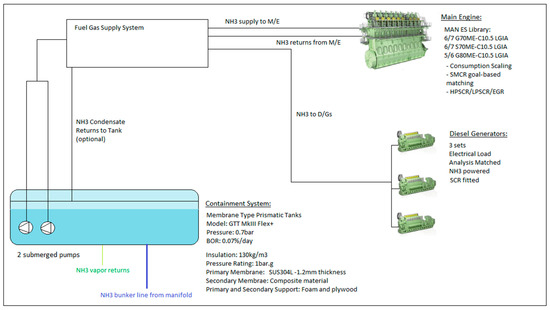
Figure 4.
Indicative P&ID of the NH3 containment, processing and consumption system.
At this point it should be highlighted that for the sake of modelling simplicity, efficiency and globality it was chosen not to examine the FGSS design but rather “macroscopically” treating it as a “black box” and modelling it as additional electrical power and steam consumer. The thermodynamic simulation of the processes in the FGSS is not considered as it is regarded as a detailed design objective. Additionally, further hybridization of the power plant with the use of batteries and a shaft generator is also not considered. Given this, the adjustment of the simulation-based RHODA methodology is herein focused on the following tasks:
- ○
- Main Engine Performance and NH3 Consumption Modelling,
- ○
- Diesel Generator NH3 Consumption Assumption,
- ○
- Containment System Capacity Sizing and Modelling,
- ○
- FGSS footprint assessment,
- ○
- CAPEX modelling,
- ○
- Probabilistic analysis of NH3 pricing,
- ○
- Definition of Maximum Ammonia Price (MAP).
2.3.1. Main Engine Performance and Consumption Modelling
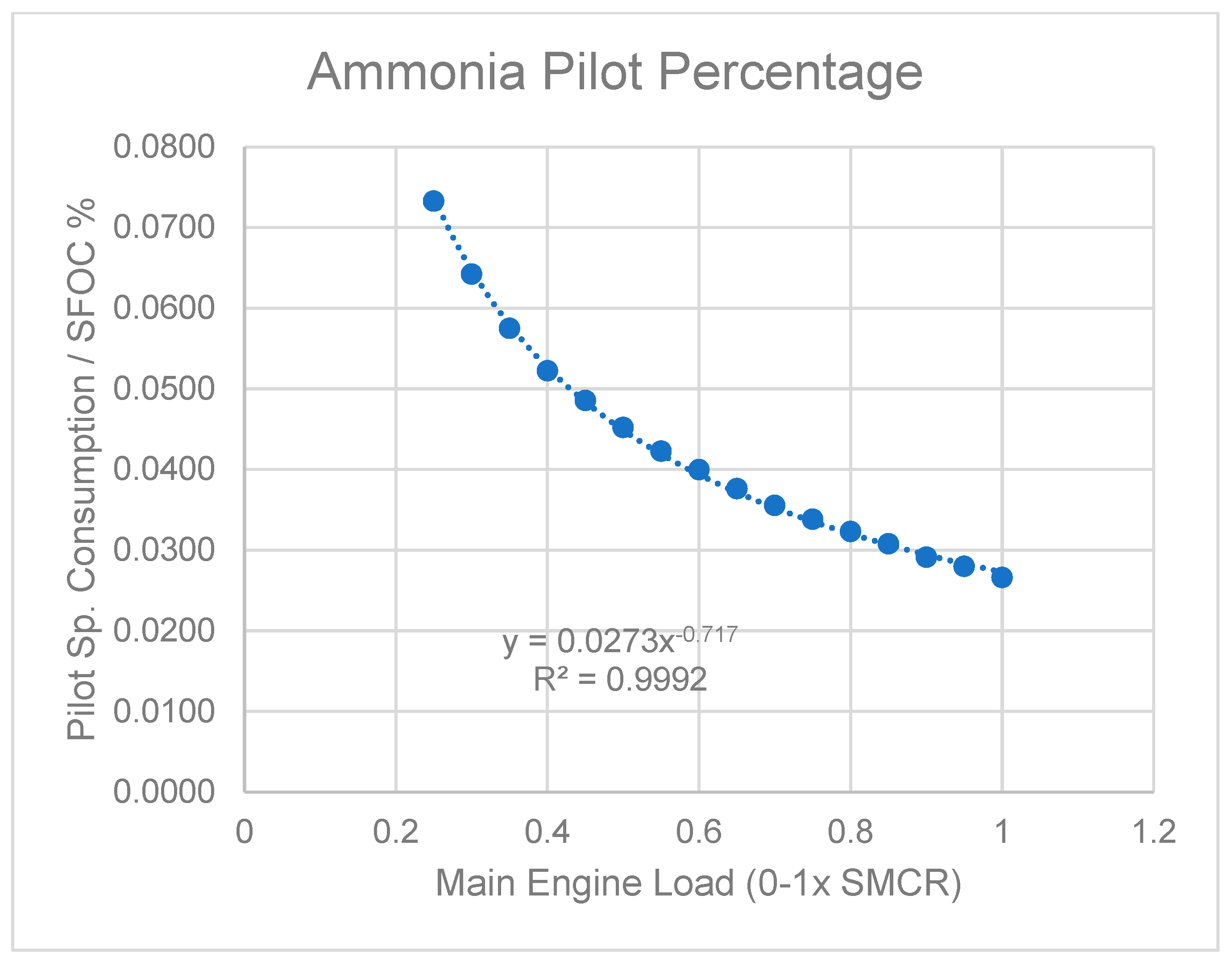
When taking into consideration the total energy balance onboard for seagoing conditions, it is straightforward that the main engine and the energy demand of the latter constitute the primary and major consumption components of any propulsion plant. For the herein presented study of the Zero Emission Vessel case study, a two-stroke engine-based propulsion plant is assumed, accompanied by four-stroke diesel engine generator sets. Effectively, the philosophy of the propulsion and engineering plant of the vessel is the use of the ammonia-fueled counterparts of the existing VLSFO-fueled components. One could argue that the use of solid oxide fuel cells could replace both propulsion and electricity generation components; however, due to the very high capital intensity of this technology, such applications were not examined. At the time of the code development and writing, there were no available two-stroke engines capable of burning ammonia in operation or as readily available designs. The only contemporary ammonia-powered engine that could be used as an analysis basis was the “ME-C-LGIA” developed by MAN [4]. The data available to the authors, however, were available only for the larger bore seven-cylinder G80 engine of MAN (800 mm bore), which is included in the methodology engine library and repository but not frequently selected by the engine–propeller matching module. Given that the same data for the same tuning are also available for the conventional, “base” engine of the G80 family (7G80ME-C10.5) and considering the thermodynamic process and the diesel cycle use of the LGIA engine [4], it was decided to define a load-dependent “scaling” function that can be used for all available engines in the RHODA engine library to convert the Specific Fuel Consumption figure (MGO basis) to Specific Ammonia Consumption (SAC). The scaling function has been modelled by deriving a logarithmic function using regression models (Figure 5), while the specific pilot consumption was defined again as a load-dependent non-dimensional function of the SAC (Figure 6). The pilot fuel is hereby assumed to be MGO or VLSFO, but in future analysis, it can be considered as biofuel instead.
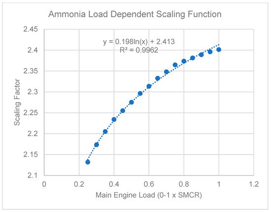
Figure 5.
Modelling of Load-Dependent Ammonia-Specific Consumption Scaling Function.
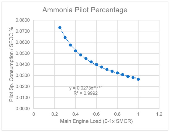
Figure 6.
Modelling of Load-Dependent Ammonia - Specific Pilot Oil Consumption as a percentage of NH3-SFOC.
2.3.2. Diesel Generator NH3 Consumption Modelling
For the purposes of the present study, the diesel generator consumption and performance modelling was modelled by scaling the VLSFO consumption curve by the scale ratio of the Lower Calorific Values (LCV) of NH3 and VLSFO, respectively.
2.3.3. Containment System Modelling
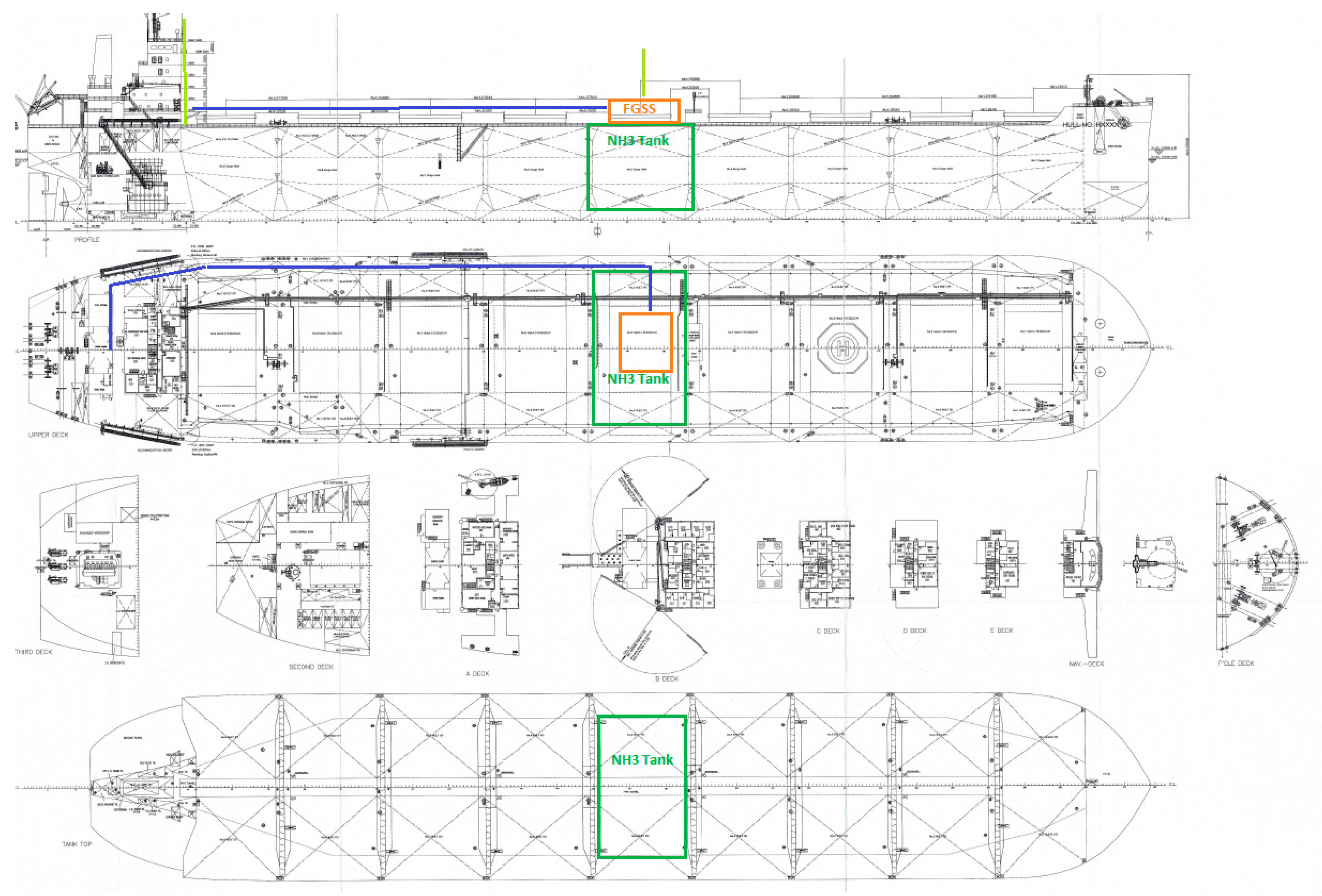
A membrane tank was chosen herein as the containment system for onboard ammonia storage. More specifically, the digital twin of the GTT Mark III Flex+ prismatic membrane tank was generated. The capacity of the membrane tank is determined as the required capacity for performing one full roundtrip of the Brazil to China trade route without re-fueling using the output of the voyage simulation code in terms of anticipated NH3 consumption for a roundtrip including the tank filling limitations and boil-of-rate of ammonia and an addition of a safety margin of 5%. Given that this is by far one of the longest routes that large bulk carriers are employed in, the calculated capacity corresponds to the worst-case scenario. The capacity of the containment system can be a separate subject of local design sensitivity analysis as examined in the discussion of optimization results. Spatially, the membrane tank center was modelled to coincide with the midship of each vessel variant and take the same parametric prismatic shape required to match the determined required capacity. The membrane tank is located within the adjacent cargo hold with a small cofferdam around the latter. For this purpose, two additional transverse bulkheads were added to the lightship model. The tank’s special gravity, capacity and longitudinal as well as the transverse center of gravity were added in the Trim and Stability module, while the fuel tanks were removed. With the above formulation, the loss of cargo as well as new loading cases were assessed. A sketch of the relevant arrangements of the ammonia bunker Tank (membrane), FGSS Room, NH3 lines and vent lines can be seen in Figure 7 below. The relevant arrangements are under the provisions of the IGF Code [26].
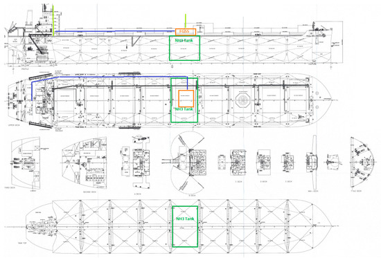
Figure 7.
Sketch of the relevant locations of the NH3 tank (green), FGSS room (orange), NH3 lines (blue) and vent lines (light green).
One of the important elements of the membrane is the cost of the latter and its effect on the additional CAPEX required for the NH3 variants. The cost was modelled parametrically as a cost (USD) per cubic meter of a capacity, and this ratio, in turn, was modelled as a linear function of the total capacity.
2.3.4. FGSS System Basic Philosophy and Sizing
The FGSS system was assumed as a black box, modelled as only an electrical and steam consumer, with a constant load (kW) and steam consumption (kg/h) assumed. As this is a preliminary ship design context exploration, it was considered sufficient.
2.3.5. Additional NH3 Handling Component CAPEX Modelling
The assessment of the additional capital expenditure to cover the cost required for the NH3 containment, processing and combustion equipment as well as safety and venting equipment is important due to its effect on RFR. The total additional expenditure is decomposed into several categories including containment system, main engine modifications, Fuel Gas Supply System (FGSS), structural reinforcements, venting and safety arrangements, etc.
2.3.6. Ammonia Pricing Probabilistic Approach to Uncertainty Modelling
As NH3 has not been used as a marine fuel in the past, there is little to no reference [27] to the pricing of the latter in such a way that the distribution and bunkering networking is accounted for. Furthermore, despite the existence of references for ammonia pricing from the heavy land-based industry (fertilizers), this is primarily for “brown” ammonia [28]. Brown ammonia, however, leaves a considerable CO2 footprint since it is typically a side product of coal-fired land power stations or from methane consumption [29]. If the GWP and CO2e tons of the same source are used for the lifecycle assessment of emissions generated on a well-to-tank basis, ammonia has a heavier carbon footprint than VLSFO. For the context of the use of ammonia in shipping decarbonization thus, only “blue” or “green” ammonia were hereby considered which are either the product of carbon-capturing or generated from alternative hydrogen and power sources. The pricing of this, with the uplift of the marine distribution network, is far from available and reliable. For this reason, a hybrid approach was employed as the first attempt to price NH3 within the context of RHODA. In the first stage, a probabilistic, weighted average method was used in the same way as in the VLSFO-based version of the methodology with the absence, however, of the probability distribution functions of the pricing. Instead, low, middle and high pricing were introduced at USD 700/ton, USD 1200/ton and USD 1800/ton, respectively. These were attributed and matched with an equal probability of occurrence of 1/3, respectively. A higher combined probability was given for the high and middle scenarios. This choice was made as in the first years of NH3 production; the unitized production is expected to be at a higher side before scaling up of electro-fuel. In addition, processes can drive the pricing down.
2.3.7. Definition of Maximum Ammonia Pricing (MAP)
A second attempt to map the pricing of NH3 was made through the introduction of a new design metric, the Maximum Ammonia Pricing (MAP). This metric was conceived by one of the authors in the preliminary assessment of NH3-powered concepts of VLCCs joint industrial projects (JIP) and inspired by the definition of the Required Freight Rate design metric. In this context, the Maximum Ammonia Price reflects the maximum allowable pricing of NH3 that will allow an NH3-powered vessel to recover the additional CAPEX as well as OPEX (due to the threefold daily consumption) within 10 years from delivery of the NH3-powered vessel (or retrofit) considering the savings realized from the reduced CO2 taxation. This is depicted in the below formula:
where
AddCAPEX is the additional CAPEX of the NH3 onboard containment, processing and combustion equipment;
Amortization is the time by which additional investment is required to be amortized;
FOC is the annual fuel cost of the VLSFO variant;
CO2 is the annual emission tax cost of the VLSFO variant;
Pilot_Cost is the annual cost of the pilot fuel amount (calculated from the simulation module);
Pilot_CO2cost is the annual taxation of the CO2 emitted from the combustion of pilot fuel.
3. Application of RHODA in Design Optimization Studies of Zero Emission Bulk Carriers
The Global Optimization Study conducted for the zero-emission vessel herein presented has been using the RHODA model in CAESES® software. The optimization engine selected was the NSGAII algorithm (Non-Sorting Genetic Algorithm II) used in previous research work [23]. The NSGAII setup based on previous experience was deployed for 20 generations of designs, with each generation containing a population of 100 designs. As a result, a total number of 1196 viable designs were generated out of a total population of 2000 designs corresponding to a 59.8% success rate. The reason for the use of a higher number (20 generations of a 100-item population size, corresponding to 2000 variants) is the positive effects of a higher number of generations in the Pareto front structure and density. The lower success rate was the result of the presence of primarily unfeasible designs (very low DWT or violations of the 1966 Loading Line Freeboard Height requirement), and not an outcome affected by the EEDI Phase 3 constraint with almost zero effect, since reduction in the EEDI was more than 80% due to the use of ammonia as a fuel. The RHODA model also included a second, vessel digital twin corresponding to the VLSFO powered counterpart of each design variant. In this way, the effect of the NH3 components on the design and optimization path as well as direct comparisons and assessments of ZEVs with theor VLSFO counterparts are feasible. Additionally, following the global optimization runs, a comprehensive sensitivity analysis with regard to the resulting Maximum Ammonia Pricing (MAP) was conducted with the following key findings:
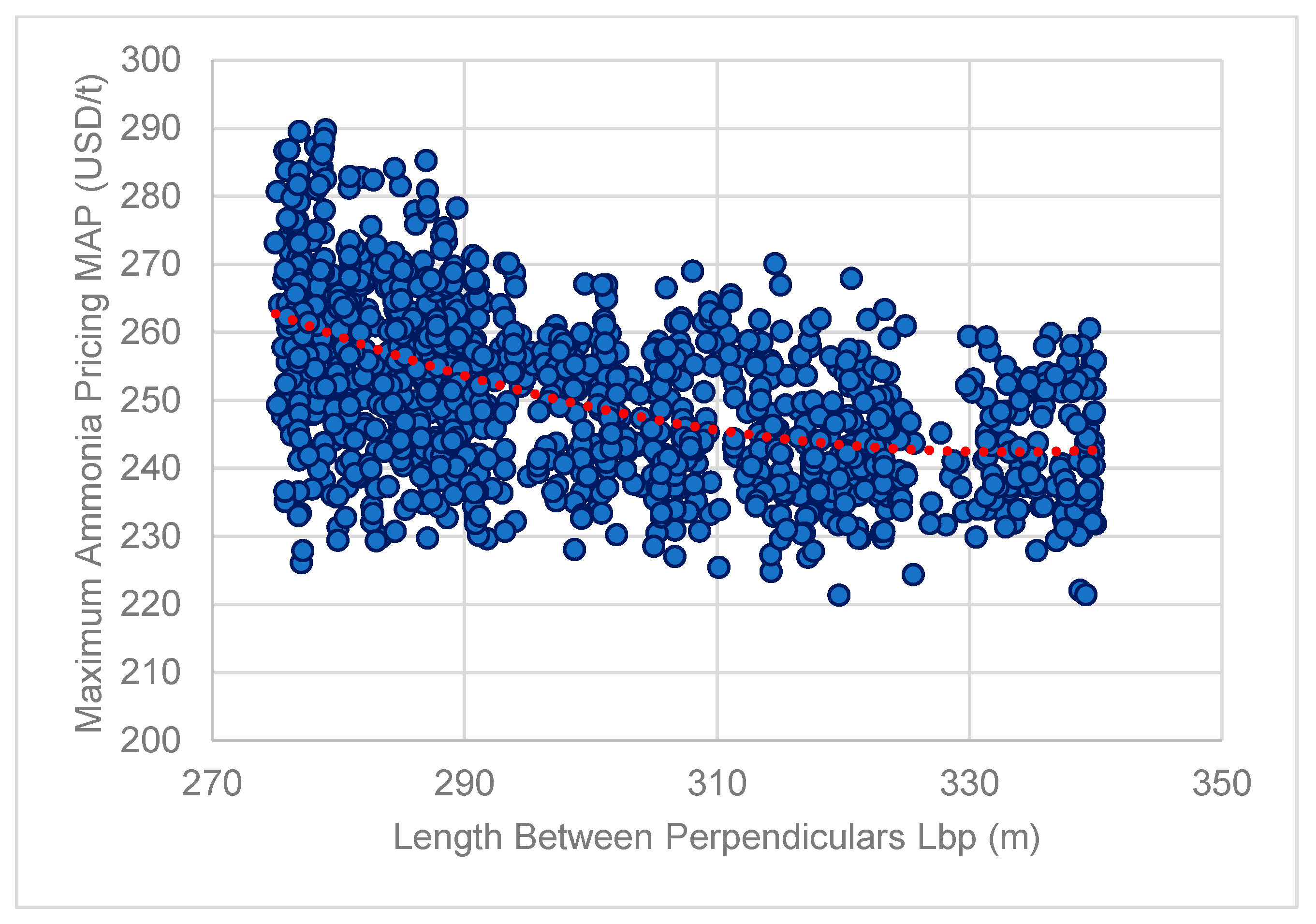
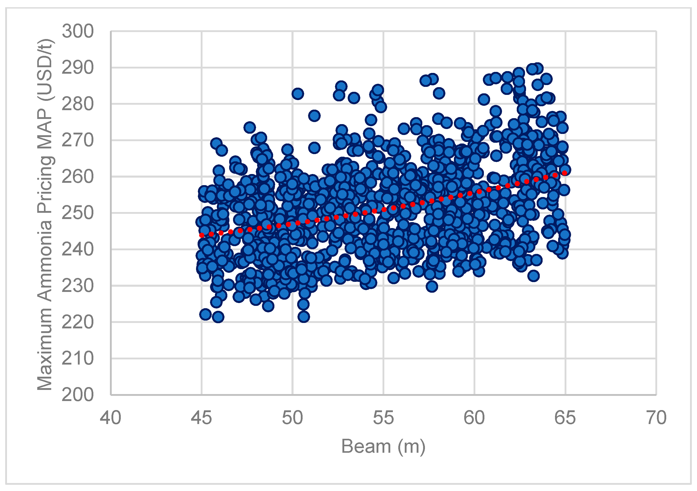
- Slender designs with short length, wide beam, deep draft and deck high have the best MAP performance, which males them the most economically viable Zero Emission Vessel variants (Figure 8, Figure 9, Figure 10 and Figure 11).
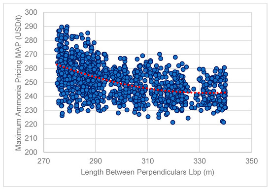 Figure 8. ZEV MAP Sensitivity on Lbp.
 Figure 9. ZEV MAP Sensitivity on Beam.
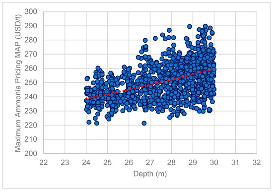 Figure 10. ZEV MAP Sensitivity on Deck Height.
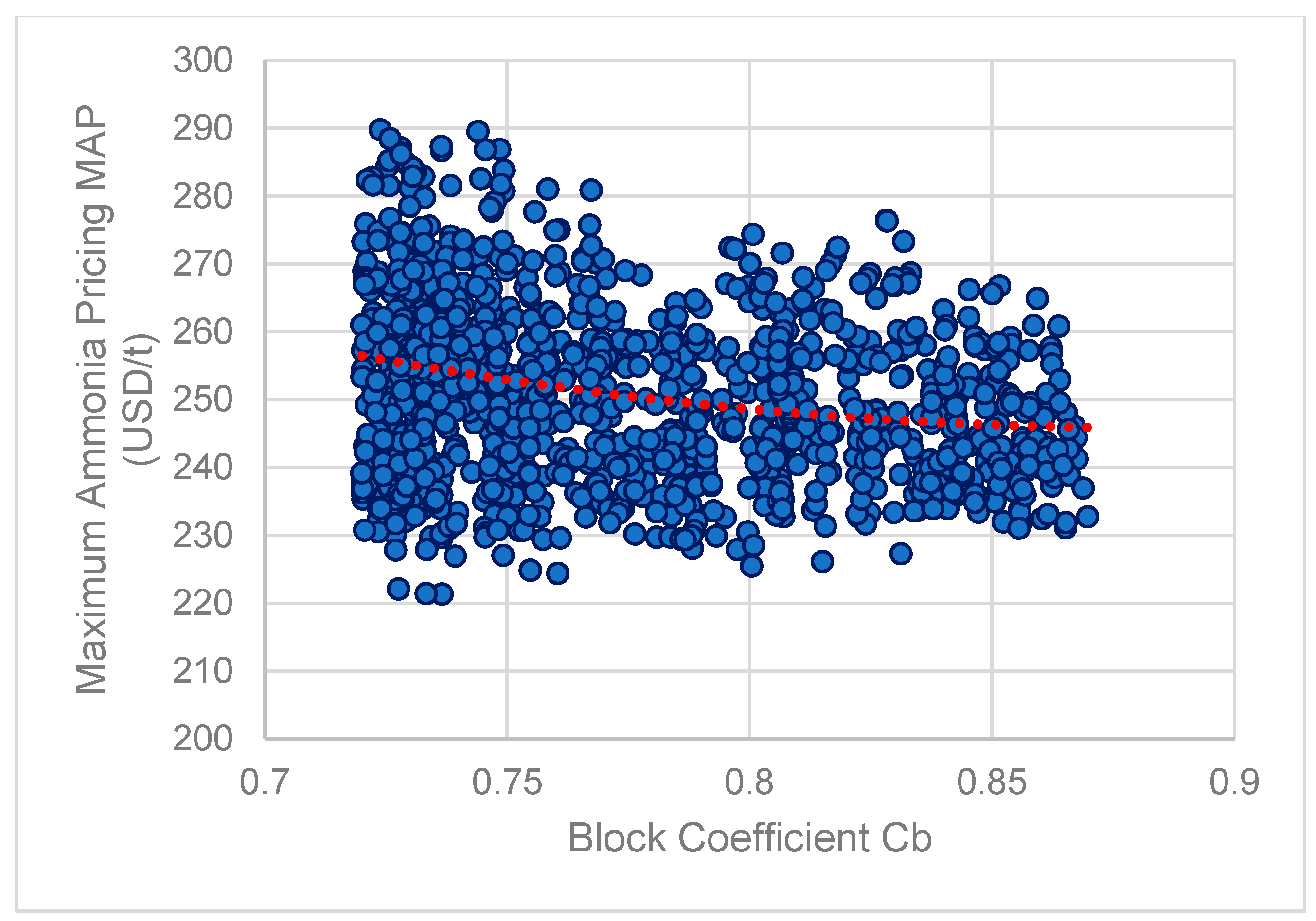
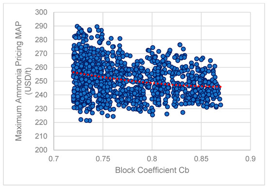 Figure 11. ZEV MAP Sensitivity on Block Coefficient.
 - Cargo Hold variables have zero effect on MAP.
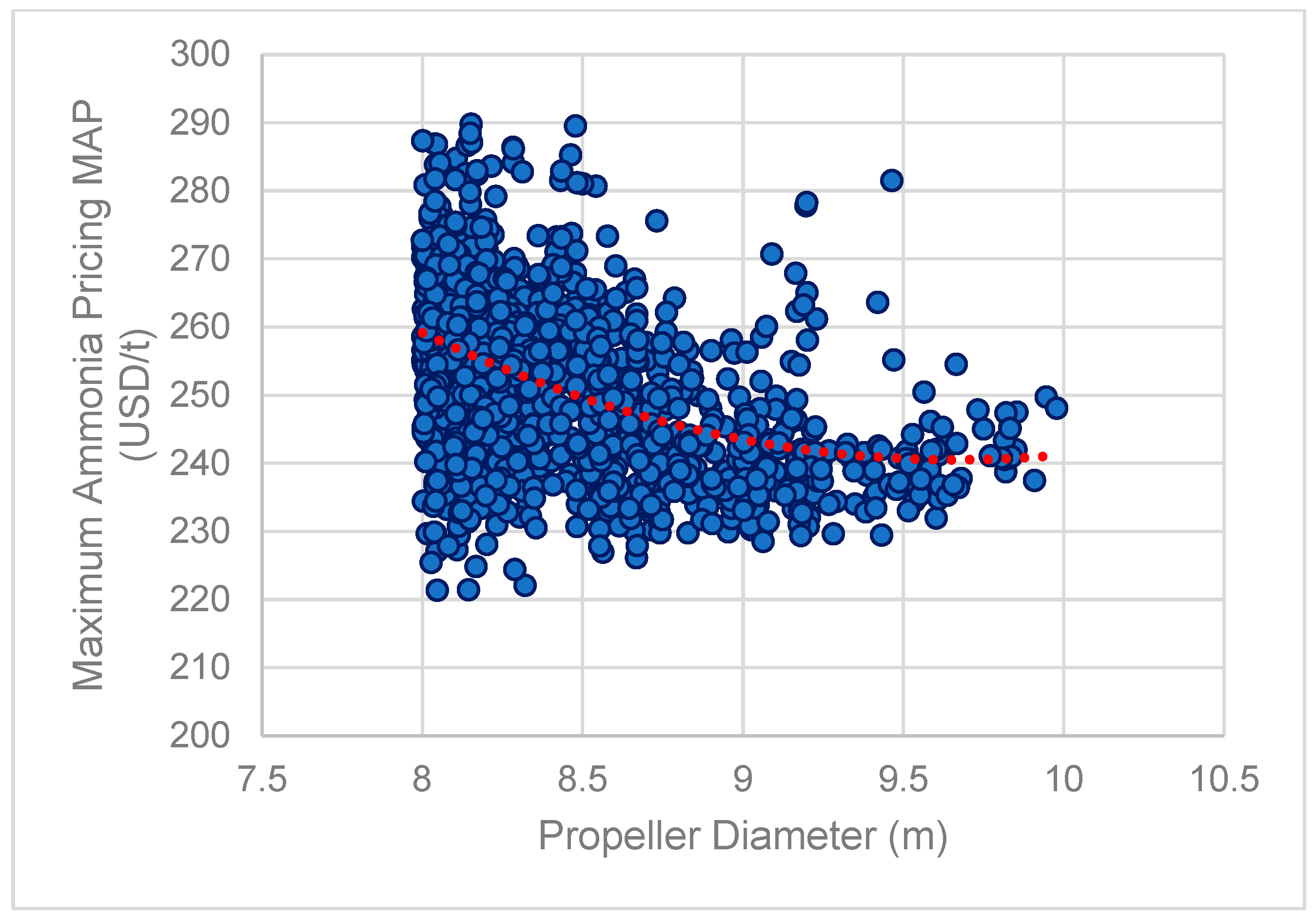
 Figure 12. ZEV MAP Sensitivity on Propeller Diameter.
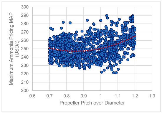 Figure 13. ZEV MAP Sensitivity on Pitch Over Diameter.
- ○
- In general, MAP is favoured by high-pitch and lower diameter propellers.
- ○
- Low Expanded Area ratio also has a positive effect on MAP (increase).
- ○
- High pitch is a typical design measure to increase efficiency and decrease installed power.
The decrease in diameter and expanded area ratio is where the algorithm is lead in order to comply with the constraints of Light Running Margin (LRM) and torque limitations of the engine.
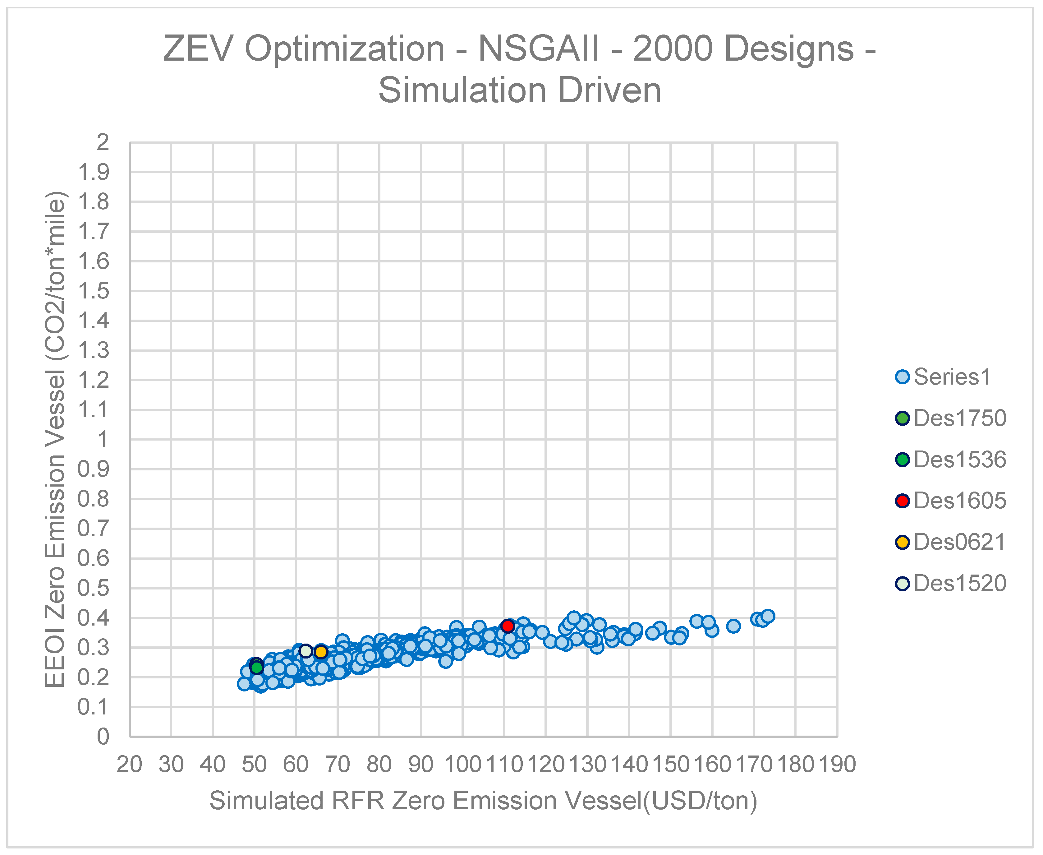
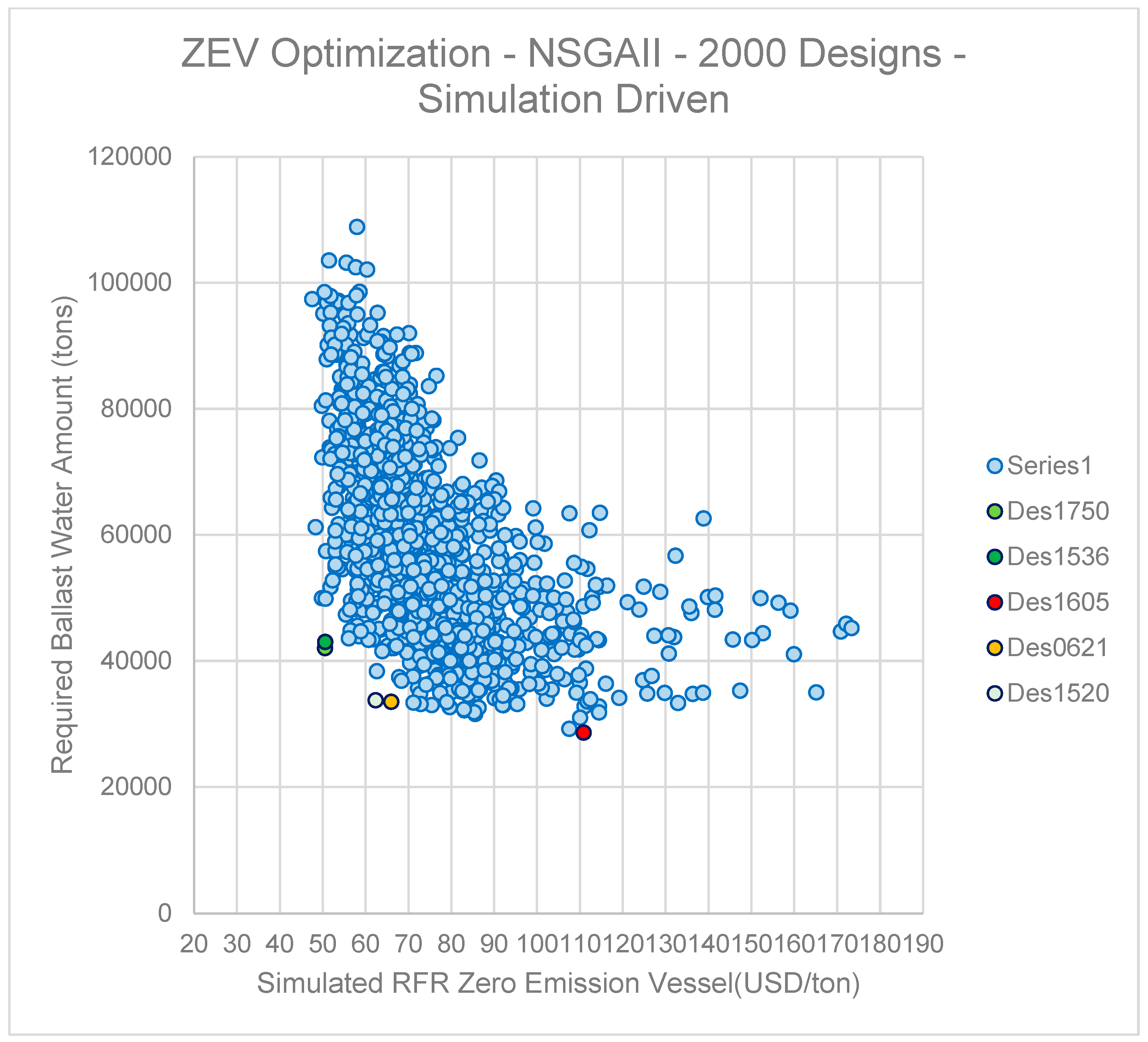
In Figure 14, the drastic reduction of the EEOI value is clearly identified. For the VLSFO counterparts of the dominant variants, the best EEOI values attained where in the region of 1.8 to 2.0 tCO2/ton × mile, while for the Zero Emission Vessel cases examined here the equivalent range was between 0.2 and 0.4 tCO2/ton × mile, corresponding to a reduction in the range of 78–90%. Such a drastic reduction contributed to the absence of carbon in the molecule of ammonia (NH3), completely removing both the EEOI and the EEDI from affecting the design decisions and sensitivities. In Figure 15, the scatter diagram comparing the simulation-based RFR for the zero-emission vessel variants and the Required Ballast Water amount is depicted. An arc-shaped Pareto frontier is observed. At the bending point of the arc, there are some offset individual designs that strictly dominate the rest of the design cloud of all adjacent regions. The ranking and pattern indicated that left-hand side regions are characterized by low RFR (and low EEOI) variants that require bigger amounts of Ballast (due to bigger dimensions) while the right-hand side is comprised of vessel variants of higher RFR (and EEOI) and drastically reduced Ballast Water amount. The most interesting region is, as previously mentioned, the area where the Pareto arc is bent. The region on its left side is comprised of a very sharp increase in the Ballast Water amount with almost negligible improvement in terms of RFR. It is therefore not a surprise that all the dominant variants resulting from all utility function scenarios are situated in the said region.
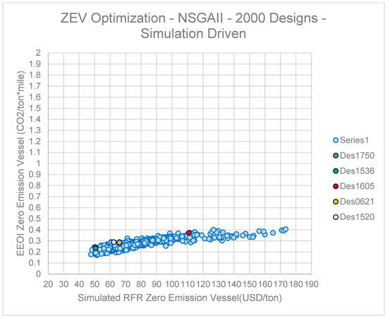
Figure 14.
Scatter Diagram of Simulation-based RFR of ZEV versus EEOI value.
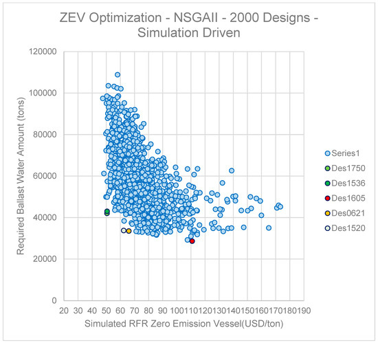
Figure 15.
Scatter Diagram of Simulation-based RFR of ZEV versus Required Ballast Water amount.
The steep end at the left-hand side of the Pareto is characteristic of the algorithm and common among similar optimization studies of the authors. The RFR minimization remains here of paramount importance, especially when considering the magnification of the latter due to the ammonia consumption (three times the amount of that of the VLSFO equivalents). The variant with the lowest Required Ballast Amount (ID1605) in this case is not to be considered for further exploration since a decrease in the Ballast amount of 33% (from 43,000 tons of the nearest dominant variant to 28,600 tons) leads to an increase in the RFR of almost twofold. When considering the already very high magnitude of the RFR (compared to conventional designs), such an increase makes the mentioned designs economically unfeasible.
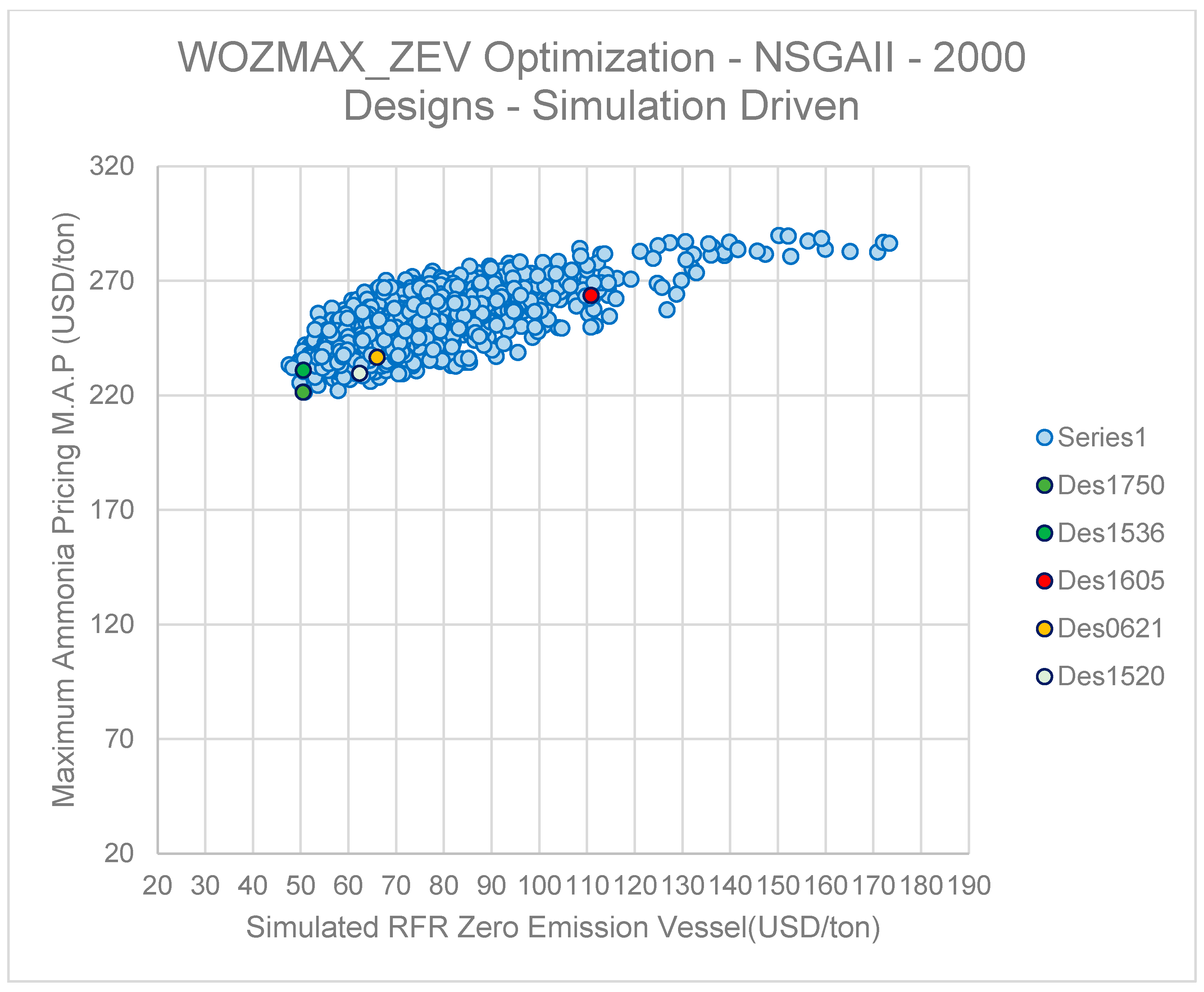
In Figure 16, the newly defined MAP scatter diagram versus the simulation-based RFR is depicted. Interestingly, despite the relatively flat shape of the scatter cloud, an upward trend of the MAP values is observed when RFR is increased. This means that design variants with a higher simulation-based RFR also have a higher MAP and thus a higher margin on the maximum allowable value of NH3 unit pricing in order to be profitable. This is explained by the fact that such designs correspond to designs that have inherently higher fuel consumption and powering requirements (both in calm sea and actual seaways), and thus their annual fuel consumption and the corresponding CO2 taxation could favor the use of NH3 instead. The reason behind this is that for a VLSFO-powered vessel, the CO2 emission factor is 3.114 [29], and thus the penalization in consumption is even harsher when CO2 taxation is considered. This trend is validated by Figure 17 and the scatter diagram between MAP and the Required Time Charter Equivalent Daily rate.

Figure 16.
Scatter Diagram of Simulation-based RFR of ZEV versus Maximum Ammonia Pricing (MAP).
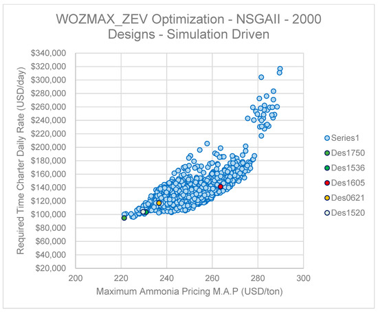
Figure 17.
Scatter Diagram of Maximum Ammonia Pricing versus Required TCE Daily Rate.
For this case, the relationship between simulation-based Required TCE Rate and MAP is much clearer. Increase in MAP increases the required TCE following a second- to third-order power curve. This relationship is stronger as the simulation-based Required TCE is supposed to cover all fuel and CO2 taxation costs over the period of the charter among other economic coverages. The number and magnitude of the MAP are also converging with the calculations performed for VLCCs in industrial studies (region of USD 300/ton), which are larger- and higher-consuming vessels than the examined bulk carriers. This offers a preliminary estimation of where the NH3 bunkering market should move in order for the latter to make an attractive business case. The validity and utility of RFR as a design metric are re-verified in Figure 18, representing the scatter diagram between the simulation-based Required TCE Daily Hire Rate and the simulation-based RFR. These two metrics indicate a strong and linear correlation of the medium inclination tangent.
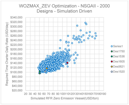
Figure 18.
Scatter Diagram of Simulation-based RFR of ZEV versus Required TCE Daily Rate.
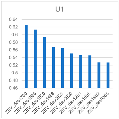
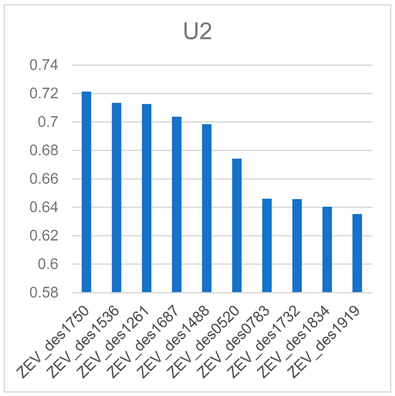
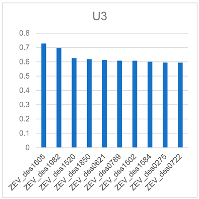
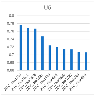
A critical part of the optimization process is the selection and ranking of dominant variants from a Pareto frontier with regard to their fit to the merits set as optimization targets. In view of this, the technique of utility functions is deployed on the respective Pareto frontiers. For the engineering problem herein examined, the desirable merits of the generated designs are minimum EEOI, RFR and Required Ballast Amount. Instead of using fixed weights for the set optimization targets in the evaluation of the variants, a utility function of the following formulation is rather assumed:
The utility of each design variant with regard to the optimization targets is normalized by the best attained value of each design population. The weights assigned for each respective KPI of each variant follow a linear distribution as a function of the distance of the attained utility value to the maximum utility value (under normalization, it has a value of 1) of the design population. In Table 3 that follows, the most favorable designs are ranked and presented for each weight scenario, resulting in the identification and sorting of a design pool (50 variants) of the best performance variants.
Table 3.
Weights used for the utility functions.
When looking at the generated design pool, an interesting observation is that the top three ranked designs among all scenarios are alternating, but the results are very similar with Design 1750 being the top-ranking variant for three out of four scenarios, indicating a very robust performance in the Pareto front. By weighing in the Pareto front relevant location, the consistent top three ranking Designs 1750, 1536 and 1520 and their combined RFR, EEOI and Ballast Water amount performance were selected as the top three optimization designs. It should be noted at this point that the selection is subject to each individual decision-maker criteria, and the goal of the global optimization studies herein presented is not the selection of one dominant design rather than the creation of a design pool comprised of the top Pareto performers (Table 4).
Table 4.
Consolidated results of Pareto Designs Ranking for 4 different utility scenarios.
The principal particulars of this selected group of dominant variants from the Simulation-Based Optimization Pathway runs applied to Zero Emission Vessels can be found in Table 5. It should be highlighted that the role of RHODA with a simulation-based assessment for actual operating speeds is quite important in order to explore the new local minima and robust solutions considering vessels that are NH3-powered by design (not just NH3-powered versions of existing designs), with each variant, however, compared to its conventional counterpart as well. With this “synchronous” optimization approach, it is possible to capture the different algorithm responses, optimization effect, Pareto front formations, dominant variant characteristics and overall pathway result for a Zero Emission Vessel against its VLSFO-powered counterpart.
Table 5.
Principal Particulars of Dominant Variants of Zero Emission Bulk Carriers.
An analysis for the principal particulars of the optimal Zero Emission Vessels produced interesting observations that can be expanded in future general Design considerations and guidelines for Zero Emission Vessels.
3.1. Observed Length
The best performers in terms of RFR have higher LBP values but are closer to the middle of the variable range, with the shortest designs being the ones with the minimized Required Ballast Water amount. The isolation and decoupling of EEOI from the optimization objectives (since the current case study concerns vessels designed for NH3 fuel) lead to a relevant relaxation of the requirements for the length, so the optimized RFR and Ballast Water amount values were found more efficiently.
3.2. Observed Beam
Interestingly, the beam of dominant variants was restrained below the 50 m threshold, which is lower than the results of the simulation-based optimization runs of VLSFO counterparts. The reason for this is that the EEOI has been lifted as an optimization objective (depolarizing the Pareto frontier from “best performer” designs).
3.3. Observed Draft
Similarly to the length, the decoupling of EEOI from the optimization targets and thus relaxation on the requirement from common minimization of both RFR and EEOI, combined with the simulation-based calculations at actual operating speeds, leads to solutions that are Pareto optimal without the need of maximizing the scantling draft.
3.4. Observed Block Coefficient (Cb)
A very interesting finding for the observed values of the block coefficient of dominant variants is that all designs are pushed at the lowest boundary of the range of block coefficient at values in the range of 0.72–0.75, which is not common in actual shipbuilding practice. Interestingly, the reduction in the Cb for simulation-based studies, apart from reducing the installed power of the main engine, drastically reduces the added resistance in actual seaways and for the most frequent operating speeds of the specific trade routes examined.
3.5. Observed Deck Height
The Deck height of the dominant variants was found to be the middle (instead of upper) bound of the variable range, with most dominant variants displaying a height between 26 and 27 m. Since the deck height actively contributes to the increase in the lightship and thus the building cost and initial CAPEX and, consecutively, RFR on the one hand, and the current case study concerns CAPEX-intensive vessels (due to the increased CAPEX from NH3 application) on the other hand, the deck height of the dominant was restrained in this case by the algorithm in order to prevent the overshoot of the CAPEX value resulting in RFR penalization with an adverse effect on the optimization effect.
3.6. Observed Propeller Particulars
Considering the RHODA structure and voyage simulation core, propeller particulars play a very decisive role in the optimization process. As a result, the following effects from voyage simulation are observed for the propeller geometry:
- -
- Reduction in dominant variant propeller diameter;
- -
- Reduction in Expanded Area Ratio (Ae/Ao);
- -
- Increase in propeller Pitch over Diameter ratio (PoD);
- -
- More frequent dominant variants with four instead of five blades.
The reason for limited propeller diameters for dominant variants is that the aft draft in the light ballast condition is reduced and so is the required ballast amount to attain the latter load line. The simulation-based optimization here ensures the increase in propeller efficiency for the actual speeds (and thus advance coefficients J) by leading to designs of increased propeller pitch but of relatively smaller expanded area ratio to maintain a sufficient light running margin (also ensured through the engine selection module).
In Table 6, the improvement of the key optimization targets for the dominant variants of the simulation-driven pathway run for the Zero Emission Vessel case study is depicted.
Table 6.
Improvement of Optimization Targets for Dominant Variants.
The lifecycle CO2 emissions are reduced dramatically by design due to the NH3 powered concept, with 10% of residual emissions accounted for by the pilot fuel used for the main engine and diesel generators as previously explained. The most efficient design appears to be Design ID1750, which features a reduction in RFR by 14.1% for the NH3 variant which corresponds to a reduction of 8.50% for the VLSFO-powered equivalent. In the meantime, the EEOI is further reduced by 17.19% when compared to the baseline, contributing as well to CO2 reduction. The Required TCE is improved by 13% when compared to the baseline. Design ID1536, which has the same level of RFR improvement for the NH3-powered variant, has a similar valueit, while the simulation-based RFR of the VLSFO variant is further reduced by 10% when compared to the baseline. The most interesting observation here, however, is that for both “best performers” there has been no penalization at all with regard to the Required Ballast Water amount. On the contrary, both designs feature an almost 40% reduction of the Ballast Water amount.
4. Discussion
From previous analysis (Table 5 and Table 6), it is evident that all ZEV variants illustrate a remarkably high value of RFR and Lifecycle Economic performance compared to the equivalent one of the their VLSFO counterparts due to the threefold increase in consumption (due to the very low energy density of NH3 and concurrent high price). It should be noted, on the other hand, that these designs are the best possible performers, and compared to the other design variants they have drastically improved economic performance. Considering the need for creating Zero Emission Vessels that are also economically sustainable, a deep dive in the economic fundamentals of decarbonization follows with an extensive discussion and post-processing analysis.
4.1. What Is the True Cost of Decarbonization?
In order to assess the cost of decarbonizing the supply chain that large bulk carriers are employed in, given that the optimization results are based on dynamic simulation of voyages over each vessel’s entire lifecycle where all key economic metrics are calculated, there is a straightforward analysis for comparing the Total Cost of Ownership (TCO) discounted to Net Present Value (NPV) between the NH3-powered vessel and its VLSFO counterpart that has been concurrently calculated in the simulation module. Indeed, this was performed and presented in Table 7, where it is evident that the cost to decarbonize the baseline vessel is an additional USD 428,378,701 to the discounted TCO, whereas the cost to decarbonize ID1750 is an additional USD 336,155,660 to the discounted TCO. It thus significant to mention at this point that the application of the RHODA methodology lead to a reduction of USD 92,223,041 of decarbonization cost (21.5%) and an overall 18.48% reduction in the discounted TCO of the NH3-powered vessel.
Table 7.
Comparison of Total Cost of Ownership of Baseline and Optimized Variants.
4.2. What Is the Global Effect of the Attained CO2 Reduction If Applied to the Entire Population of Large Bulk Carriers?
The CO2 emissions of the global commercial vessel fleet have been examined systematically in [30]. In this study, the annual CO2 emissions of the entire fleet of Dry Bulk Carriers corresponds to a total of 151.03 million tons of CO2, with large bulkers herein studied (above Panamax size) producing a footprint of 36.27 million tons of CO2. If the EEOI reduction of 89.78% that was witnessed for Sim_WOZMAX_03_ID1750 is assumed as the basis, then the global effect of applying such designs across the supply chain would be the elimination of 32.56 million tons of CO2 per annum and 814.08 million tons of CO2 for a lifecycle of vessels (25 years). In order to put this reduction into scale and perspective, in 2019, the annual emissions of the entire country of Scotland were 47.8 million tons of CO2e [31], the annual emissions of the entire United Kingdom were 468 million tons [32], and for the entire world the value was 36,700 million tons of CO2e [33].
4.3. How Improving the RFR by One USD/ton Changes the Total Cost of Ownership (TCO)?
For ID1750, the total Net Present Value (NPV) of the Total Cost of Ownership (TCO) as derived from the lifecycle simulation is USD 527,808,087 and a simulation-based RFR of USD 50.554/ton. The VLSFO equivalent vessel of ID1750, in turn, has a TCO NPV of USD 191,652,427 and a simulation-based RFR of USD 16.75/ton (Table 8). The equivalent values for the baseline design are TCO NPV USD 647,468,102 and RFR USD 58.875/ton for the NH3-powered and TCO NPV USD 219,089,401 and RFR USD 18.31/ton for the VLSFO counterpart. Therefore, it can be deduced that while “navigating” on the Pareto frontier of the NH3-powered designs, a difference/increment of one USD/ton of RFR among dominant variants would translate to USD 14,380,485 of the discounted Total Cost of Ownership. Similarly, for a VLSFO-powered vessel, an RFR difference of one USD/ton among design candidates would correspond to USD 17,587,573 of the discounted Total Cost of Ownership.
Table 8.
Sensitivity Analysis of Total Cost of Ownership and Required Freight.
4.4. What Would Be the Necessary Carbon Tax Rate to Offset the Additional NH3 Costs?
Another interesting question that is very relevant currently is the following: What would be the necessary carbon tax in order to offset the rise of the TCO both for the baseline and the selected dominant variant? This requires a simple calculation of dividing the rise of the discounted TCO between the VLSFO- and NH3-powered variants of each case (baseline and dominant) by the abated tons of CO2, respectively, with the results shown in Table 9.
Table 9.
Required Carbon Taxation for Offsetting Additional Costs of ZEVs.
When seeing the derived required CO2 tax to offset the TCO increase for NH3-powered variants, it is very interesting to compare it with the CO2 tax probabilistic values assumed in the herein presented studies of USD 50, 100 and 200/ton scenarios, respectively. In general, it is a number higher than any assumption currently in the industry, and it can be used as a benchmark for carbon levy studies. An extensive discussion of the carbon taxation and market-based measures can be found in the literature, specifically in [34,35].
4.5. What Would Be the Effect on RFR by Prolonging the Vessel’s Age?
The next major design question is that of the Design Lifetime of the vessel. When looking at ships that are capital intensive (e.g., LNG Carriers, Cruise and Passenger Ships, etc.), it can be observed that they typically have a (structural) design life of 40 years that in most cases coincides with the commercial life of the vessel. The purpose of targeting such prolonged vessel lifetimes is to spread the capital expenditure over a longer period of time and in the meantime prolong the years of operation and thus income in order to lead to maximization of NPV. Due to the significant increase in the required additional CAPEX in order to invest in an NH3-powered vessel to achieve zero emissions, this is one of the sensitivities that need to be taken into account in order to prolong the vessel’s lifetime as a technique for creating a more attractive RFR.
What can be seen in Table 10 is the result of this sensitivity examination. For ID1750, the lifetime of the vessel (Economic Simulation Module input) was changed from 25 to 40 years. After repeating all calculations, the RFR for the NH3-powered ZEV has shrunk considerably from USD 50.554 to 34.69/ton, corresponding to a 31.33% improvement.
Table 10.
Sensitivity Analysis of Zero Emission Vessel’s Lifetime on Required Freight.
4.6. What Is the Effect of the Containment System Capacity on the RFR? Examine the RFR Change If the Containment System Was Designed for a Single Leg of the Brazil Trade Route Instead of Roundtrip
The biggest component of the additional CAPEX for an ammonia-powered Zero Emission Vessel is the containment system used for the storage, namely the cryogenic tanks which for the herein presented case study is a single-membrane type tank.
As described in Section 2.3, the RHODA has modelled the unitized cost of the membrane tank (USD/m3 of tank) as a function of the tank capacity. Given the linearity and cost magnitude, an immediate design consideration (also common in commercial Ship Design discussions for LNG as a fuel) would be the sensitivity of the CAPEX, RFR and TCO of the ZEV asset on the Range Requirement and if additional benefits can be yielded from a smaller range. If a bunkering stop in Singapore is assumed, the simulation module is re-calculated using the half requirement for the Range value and thus resulting in a tank of a 50% capacity.
The result of this re-assessment is depicted in Table 11 below, for which a further improvement of 4.9% is achieved with the tank reduction, making the point of cost optimization through capacity restriction valid and thus highlighting the necessity of scaling up the bunkering and infrastructure network for zero emission fuels (in this case ammonia). The reason the improvement is not more significant is attributed to the economy of the scale of membrane tanks for shipbuilders, with the unitized cost per cubic meter being shrunk by the increase in capacity.
Table 11.
Sensitivity Analysis of ZEV RFR on Containment System Capacity.
5. Conclusions
In this study, a sophisticated and novel Robust and Holistic Ship Design Approach was presented using voyage simulation as a basis and subsequently deployed in the systematic optimization of Zero Emission Vessels. The presented method was also deployed on the simulation-driven optimization of a Large Bulk Carrier that is powered by NH3 with the RHODA method being adapted to cover in its modeling the ship- and fuel-specific aspects of the design of the Zero Emission Vessel configuration. The results indicated that the application of this RHODA Optimization Method has the following benefits.
- Reduction in CO2e emissions due to ZEV configuration and subsequent optimization of 88–90%. By scaling up to the level of the global fleet of bulk carriers, this annual reduction is comparable to the annual emissions of Scotland.
- Compared to their fossil-fuel-powered counterparts, ZEV display increased capital and operating costs. Through the formal optimization and RHODA approach, a reduction in Required Freight Rate on the dominant variants ranging between 10% and 15% was achieved, corresponding to a reduction of more than USD 100 million in net present value terms for the vessel’s Total Cost of Ownership over its entire lifecycle.
- Furthermore, in post-analysis, the sensitivities of the RFR and Maximum Ammonia Pricing have been examined, as well as the ways of reducing it explored. The prolonging of the ship’s Design Life from 25 to 40 years (which can be performed structurally easily) can achieve a further reduction of 32%, and the reduction in the NH3 containment system can also positively help by a 4.9% reduction.
- Reduction in Ballast Water Amount by 38–50% resulting in smaller BWTS system footprints, smaller usage of BWT spaces and energy demands.
- The sensitivity analysis performed indicates that slender vessels with shorter length, high deck height, deep draft and smaller propeller diameter and higher pitch are more favored candidates for ZEV configurations.
From the above summary of the results, it is clear that there is a high “play” on the ship design optimization prospects, indicating that high improvement potentials for Zero Emission Vessels and measures for improving the economic sustainability of such investments were extensively discussed. As a concluding remark, we stress that it is evident that for the development of Zero Emission Vessels that will be able to undertake the challenges of the commercial shipping market, it is imperative that such robust design methodologies with voyage simulations are incorporated from the early stages of the preliminary design by shipyards, classification societies and shipowners.
Author Contributions
Conceptualization, L.N. and E.B.; Methodology, L.N.; Software, L.N.; Validation, L.N.; Formal analysis, L.N.; Investigation, L.N. and E.B.; Resources, L.N.; Data curation, L.N.; Writing—original draft, L.N.; Writing—review & editing, E.B.; Visualization, L.N.; Supervision, E.B.; Project administration, E.B. All authors have read and agreed to the published version of the manuscript.
Funding
This research received no external funding.
Acknowledgments
The authors would like to express their deep gratitude to their mentor and teacher, Apostolos Papanikolaou, Ship Design Laboratory, National Technical University of Athens, whose lectures on ship design and holistic optimization have been the inspiration for this paper. Furthermore, authors would like to acknowledge the help of Star Bulk Carriers Corporation in providing valuable data from their operating fleet and reference drawings. Boulougouris work was supported by DNVGL and RCCL, sponsors of the MSRC.
Conflicts of Interest
The opinions expressed herein are those of the authors and do not reflect the views of DNVGL and RCCL.
References
- International Maritime Organization. Adoption of the Initial IMO Strategy on Reduction of GHG Emissions; IMO: London, UK, 2018. [Google Scholar]
- Papanikolaou, A.D. Ship Design, Methodologies of Preliminary Design; Springer: Dordrecht, The Netherlands, 2014. [Google Scholar]
- Getting to Zero Coallition. 2022. Available online: https://www.globalmaritimeforum.org/getting-to-zero-coalition (accessed on 1 December 2022).
- MAN B&W Ammonia Engine. MAN B&W; Ammonia Energy Association: Melbourne, Australia, 2022. [Google Scholar]
- Hannapel, S.E. Development of Multidisciplinary Design Optimization Algorithms for Ship Design under Uncertainty. Ph.D. Thesis, University of Michigan, Ann Arbor, MI, USA, 2012. [Google Scholar]
- Hannapel, S.E.; Vlahopoulos, N. Robust and Reliable Multidiscipline Ship Design. In Proceedings of the AIAA/SSMO Multidisciplinary Analysis Optimization Conference, Fort Worth, TX, USA, 13–15 September 2010; American Institute of Aeronautics and Astronautics: Fort Worth, TX, USA, 2010. [Google Scholar]
- Good, N.A. Multi-Objective Design Optimization Considering Uncertainty in a Multi-Disciplinary Ship Synthesis Model. Ph.D. Thesis, Virginia Tech, Blacksburg, VA, USA, 2006. [Google Scholar]
- Diez, M.; Peri, D. Two-Stage Stochastic Programming Framework for Ship Design Optimization under Uncertainty. 2010. Available online: https://www.academia.edu/download/39293403/54d0bebe0cf298d65668759b.pdf (accessed on 1 December 2022).
- Diez, M.; Peri, D.; Fasano, G.; Campana, E.F. Multi-Disciplinary Robust Optimization for Ship Design. In Proceedings of the 28th Symposium on Naval Hydrodynamics, Pasadena, CA, USA, 12–17 September 2010. [Google Scholar]
- Plessas, T.; Papanikolaou, A. Stochastic life cycle ship design optimization. In Proceedings of the VI International Conference on Computational Methods in Marine Engineering MARINE 2015, Rome, Italy, 15–17 June 2015. [Google Scholar]
- Plessas, T.; Papanikolaou, A.; Liu, S.; Adamopoulos, N. Optimization of Ship Design for life cycle operation with Uncertainties. In Proceedings of the International Marine Design Conference (IMDC) 2018; Taylor and Francis Group: Helsinki, Finland, 2018. [Google Scholar]
- Tillig, F.; Ringsberg, J.W. A 4 DOF simulation model developed for fuel consumption prediction of ships at sea. Ships Offshore Struct. 2019, 14, 112–120. [Google Scholar] [CrossRef]
- Tillig, F.; Ringsberg, J.W.; Mao, W.; Ramne, B. A generic energy systems model for efficient ship design and operation. J. Eng. Marit. Environ. 2017, 231, 649–666. [Google Scholar] [CrossRef]
- Alwan, S. Simulation-Based Ship Design and System Engineering. Available online: https://www.researchgate.net/publication/318044455_ENERGY_EFFICIENCY_SIMULATION-BASED_SHIP_DESIGN_AND_SYSTEM_ENGINEERING (accessed on 1 December 2022).
- Sandvik, E.; Asbjørnslett, B.E.; Steen, S.; Johnsen, T.A.V. Estimation of fuel consumption using discrete-event simulation—A validation study. In Proceedings of the International Marine Design Conference (IMDC) 2018, Helsinki, Finland, 10–14 June 2018; Taylor and Francis Group: Helsinki, Finland, 2018. [Google Scholar]
- Aristotle; Ross, W.D. Aristotle’s Metaphysics; Clarendon Press: Oxford, UK, 1981. [Google Scholar]
- Papanikolaou, A. Holistic ship design optimization. Comput.-Aided Des. 2010, 42, 1028–1044. [Google Scholar] [CrossRef]
- Papanikolaou, A. Holistic Ship Design Optimization. In A Holistic Approach to Ship Design—Volume 1: Optimization of Ship Design and Operation for Life Cycle; Papanikolaou, A., Ed.; Springer: Athens, Greece, 2019; pp. 9–42. [Google Scholar]
- Papanikolaou, A. Holistic Approach to Ship Design. J. Mar. Sci. Eng. 2022, 10, 1717. [Google Scholar] [CrossRef]
- Papanikolaou, A.; Zaraphonitis, G.; Boulougouris, E.; Langbecker, U.; Matho, S. Multi-Objective Optimization of an AFRAMAX Oil Tanker Design. J. Mar. Sci. Technol. 2010, 15, 359–373. [Google Scholar] [CrossRef]
- Papanikolaou, A.; Tuzcu, C.; Tsichlis, P. Risk-Based Optimization of Tanker Design. In Proceedings of the 3rd International Maritime Conference on Design for Safety, Berkeley, CA, USA, 8–10 February 2007. [Google Scholar]
- Nikolopoulos, L.; Boulougouris, E. A Methodology for the Holistic, Simulation Driven Ship Design Optimization under Uncertainty. In Proceedings of the International Marine Design Conference, Espoo, Finland, 10–14 June 2018. [Google Scholar]
- Nikolopoulos, L.; Boulougouris, E. A novel method for the Holistic, Simulation Driven Ship Design Optimization under uncertainty in the Big Data Era. Ocean. Eng. 2020, 218, 107634. [Google Scholar] [CrossRef]
- ISO15016; Ships and Marine Technology—Guidelines for the Assessment of Speed and Power Performance by Analysis of Speed Trial Data. International Organization for Standardization: Geneva, Switzerland, 2015.
- Clarksons Shipping Intelligence. Clarksons Shipping Intelligence Database. 2015. Available online: https://sin.clarksons.net (accessed on 1 December 2022).
- IMO. International Code of Safety for Ships Using Gases or Other Low-Flashpoint Fuels (IGF Code); IMO: London, UK, 2017. [Google Scholar]
- S&P Platts. 2022. Available online: https://www.spglobal.com/commodityinsights/en/about-commodityinsights/media-center/press-releases/2022/042622-sp-global-commodity-insights-launches-platts-ammonia-forward-curve-assessments (accessed on 1 December 2022).
- Fertecon. Fertecon Price Methodology; IHS Markit: London, UK, 2020. [Google Scholar]
- European Commision. Regulation of the European Parliament and of the Council on the Use of Renewable and Low-Carbon Fuels in Maritime Transport Ammending Directive 2009/16/EC; European Commission: Brussels, Belgium, 2021. [Google Scholar]
- Psaraftis, H.N.; Kontovas, C.A. CO2 Emission Statistics for the World Commercial Fleet. WMU J. Marit. Aff. 2009, 8, 1–25. [Google Scholar] [CrossRef]
- Statista. Statista. 2022. Available online: https://www.statista.com/statistics/367892/greenhouse-gas-emissions-scotland-annually/ (accessed on 1 December 2022).
- Annual Volume of Carbon Dioxide (CO2) Emissions in the United Kingdom (UK)* from 1990 to 2020. Statista. 2022. Available online: https://www.statista.com/statistics/486129/co2-emission-uk/ (accessed on 1 December 2022).
- Annual Carbon Dioxide (CO2) Emissions Worldwide from 1940 to 2022. Statista. 2022. Available online: https://www.statista.com/statistics/276629/global-co2-emissions/ (accessed on 1 December 2022).
- Psaraftis, H.N.; Zis, T.; Lagouvardou, S. A comparative evaluation of market based measures for shipping decarbonization. Marit. Transp. Res. 2021, 2, 100019. [Google Scholar] [CrossRef]
- Psaraftis, H.N. Shipping decarbonization in the aftermath of MEPC 76. Clean. Logist. Supply Chain. 2021, 1, 100008. [Google Scholar] [CrossRef]


Disclaimer/Publisher’s Note: The statements, opinions and data contained in all publications are solely those of the individual author(s) and contributor(s) and not of MDPI and/or the editor(s). MDPI and/or the editor(s) disclaim responsibility for any injury to people or property resulting from any ideas, methods, instructions or products referred to in the content. |
© 2023 by the authors. Licensee MDPI, Basel, Switzerland. This article is an open access article distributed under the terms and conditions of the Creative Commons Attribution (CC BY) license (https://creativecommons.org/licenses/by/4.0/).