Abstract
Forecasting peak electrical energy consumption is important because it allows utilities to properly plan for the production and distribution of electrical energy. This reduces operating costs and avoids power outages. In addition, it can help reduce environmental impact by allowing for more efficient power generation and reducing the need for additional fossil fuels during periods of high demand. In the current work, electric power consumption data from “Compagnie Electrique du Benin (CEB)” was used to deduce the peak electric power consumption at peak hours. The peak consumption of electric power was predicted using hybrid approaches based on traditional time series prediction methods (autoregressive integrated moving average (ARIMA)) and deep learning methods (long short-term memory (LSTM), gated recurrent unit (GRU)). The ARIMA approach was used to model the trend term, while deep learning approaches were employed to interpret the fluctuation term, and the outputs from these models were combined to provide the final result. The hybrid approach, ARIMA-LSTM, provided the best prediction performance with root mean square error (RMSE) of 7.35, while for the ARIMA-GRU hybrid approach, the RMSE was 9.60. Overall, the hybrid approaches outperformed the single approaches, such as GRU, LSTM, and ARIMA, which exhibited RMSE values of 18.11, 18.74, and 49.90, respectively.
1. Introduction
The production of electricity must meet the demand of consumers. Therefore, based on consumer demand, the electrical system must instantly adjust its level of electricity production and meet consumer demand without any shortages or wastage. Consequently, producing electricity to meet consumer demand is a truly challenging operation because electricity cannot be easily stored. A way to forecast future demand during peak hours would be highly beneficial for electrical grid operators when deciding on the electricity production model, thereby allowing the system to improve the quality and reliability of electricity. Electrical grid operators can then decide to rely on their own generators or seek another independent electricity producer to meet the demand, such as the Electricity Company of TOGO, which also relies on certain independent electricity producers.
Following the increasing interest in artificial intelligence (AI) and machine learning (ML), several forecasting models have been used worldwide to estimate electricity consumption. These include single models, ensemble models, and hybrid models. The time horizons for these models are as follows: very short-term for load and frequency control and economic dispatch functions [1,2,3], short-term for daily operations of electrical systems, medium-term for generator scheduling, and long-term for the construction of new transmission lines and substations for system improvement. The forecast periods for very short-term, short-term, medium-term, and long-term range from a few minutes to an hour, from an hour to a week, from a week to a year, and from a year to a decade, respectively [3].
In Slovakia, Pavlicko et al. proposed models for forecasting the daily maximum hourly electricity consumption that are more accurate than the official load forecasts of the Slovak distribution company [4]. In their publication, they present and compare different models. The first group of models is based on the cross-sectional ensemble of grey models and nonlinear Bernoulli grey models. The second approach is based on a feedback multilayer backpropagation neural network.
In recent years, many prediction techniques, including fuzzy logic, neuro-fuzzy, logistic regression, random forest, support vector machines, and artificial neural networks have been proposed. In the context of short-term load forecasting, Cao et al. adopted the hybrid decision model based on ARIMA (autoregressive integrated moving average) and similar day method for daily load forecasting in households. Their results showed that the hybrid method performed well compared to the individual basic methods [5]. Guo Fend et al. used the Empirical Mode Decomposition (EMD) method, Support Vector Regression (SVR) model, Particle Swarm Optimization (PSO) algorithm, Thermal Reaction Dynamics (TRD) theory, and an econometric model (AR-GARCH model) to develop a new hybrid forecasting model, namely the EMD-SVR-PSO-AR-GARCH model, to forecast electricity consumption [6]. Karin Kandananond used the artificial neural network approach (ANN) to predict electricity demand in Thailand [7]. This author adopted a comparative approach with other old methods such as ARIMA and multilinear regression, and found the ANN approach was the best. In Togo, Guenoukpati et al. used three machine learning approaches, namely, Support Vector Regression (SVR), the multilayer perceptron (MLP) approach, and a long short-term memory (LSTM) recurrent neural network to predict the electricity production of the Benin Electricity Community. The results of their work argue that machine learning methods offer better results than linear regression methods and are better suited for short-term predictions [8]. Yalcinoz et al. also used MLP to predict medium0 and short-term electrical load in Turkey [9]. Three load prediction modules were developed using feedforward neural networks. The neural networks were trained to recognize the day’s peak load, the day’s total load, and the monthly power consumption. In their work, Xion et al. proposed a new GM (grey model) (1,1) based on the initial condition optimization, according to the principle of new information priority, to model and predict energy consumption and production in China [10]. This new model was compared to five other GM models. The results show that the optimized model performs better than the other five models. Furthermore, in the literature, hybrid approaches involving statistical and neural models have been proven. Manowska et al. predicted the consumption of natural gas in Poland for the year 2040 with the hybrid ARIMA-LSTM approach. This approach was validated with a percentage error of 2% [11]. Zhou et al. used the mixture of integrated wavelet decomposition, autoregressive integrated moving average (ARIMA), and a managed recurrent unit (GRU) model, abbreviated as the W-ARIMA-GRU model, to predict the water quality. The results were satisfactory, with an accuracy of more than 97% [12].
Several research works have been conducted to compare forecasting models and determine which ones perform best in predicting peak electricity demand. Different studies have been conducted to identify the best performing models to anticipate these peaks in electricity demand. Several of these studies have been especially conducted on buildings [13,14] and few are oriented to territorial consumption. In particular, in Togo, no work has been undertaken in the framework of forecasting the peak consumption of electricity. Therefore, the aim of the current work is to fill this gap.
In this paper, we study five approaches, one of which is based on the statistical model applied to time series (ARIMA), two on neural models (LSTM and GRU), and the remaining two on hybridization (ARIMA-LSTM and ARIMA-GRU).
2. Data
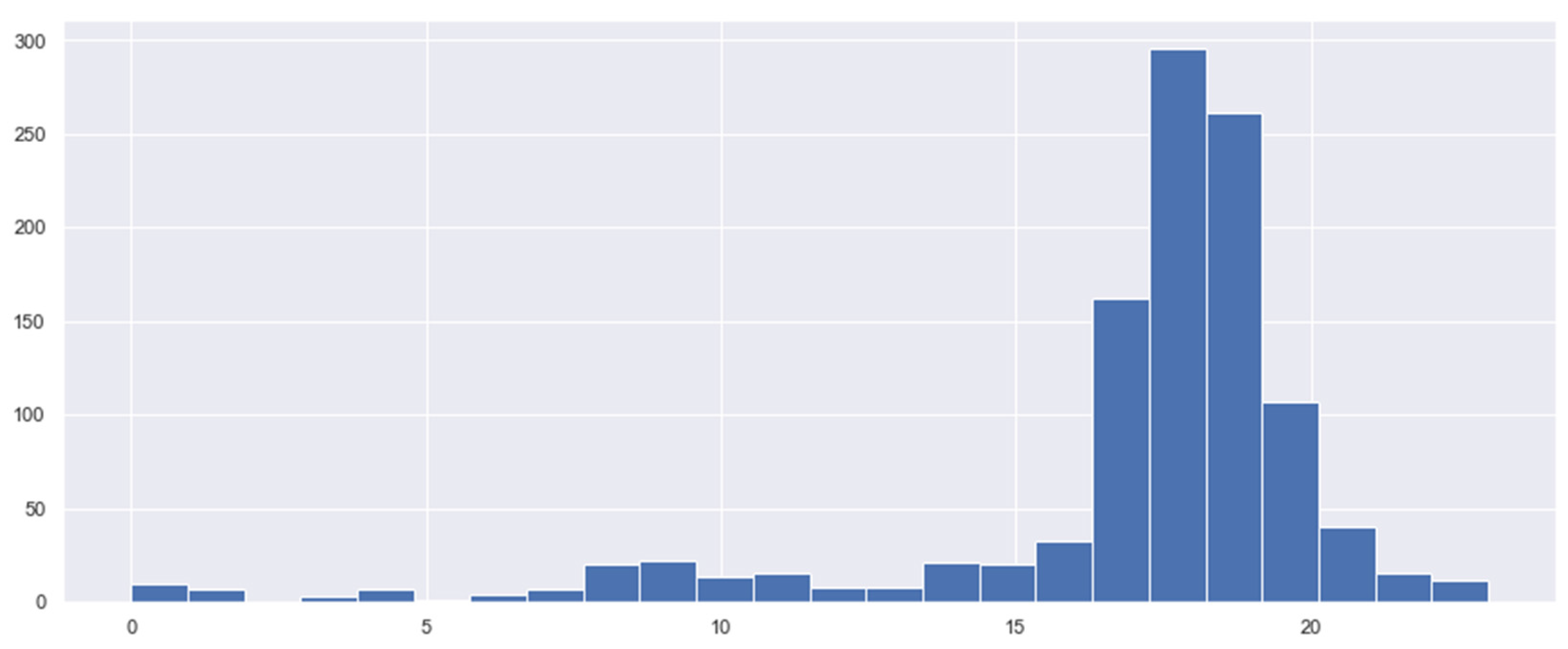
The electricity demand data are provided by the Benin Electricity Company (CEB). These data include the daily demand for electrical energy from the population over a period of four (04) years. The data are collected at hourly intervals at the CEB recording station. The daily peak demand is therefore the maximum recorded within a 24 h period. Since our study focuses on daily consumption peaks, we performed a processing step to extract the daily peaks in order to create a new training dataset for the models. Table 1 provides a brief description of the input data. Figure 1 shows the histogram of the demand peak data. We observe that the demand peaks are more concentrated between 5:00 PM and 08:00 PM. This explains the high consumption levels in residential areas.

Table 1.
Data statistics.
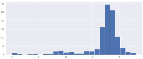
Figure 1.
Data distribution.
3. Models
Time series analysis and dynamic modeling are very diverse research areas with many applications in business, economics, finance, and computer science [15]. The objective of time series analysis is to study the path of time series observations and build a model to describe the structure of the data, and then predict future values of the time series. Due to the importance of time series forecasting in many branches of applied sciences, it is essential to build an effective model with the aim of improving the accuracy of the forecast. A variety of time series forecasting models have been developed in the literature.
3.1. LSTM
In this section we describe the long short-term memory (LSTM) recurrent neural network approach. The long short-term memory (LSTM) is a type of recurrent neural network (RNN) capable of remembering values from previous steps for future use. The main weakness of the RNN is that it is good for short-term memory but not good for long-term memory [15]. Due to the existence of the activation function (the range of output values [0,1]), when the information and residuals are transmitted into the RNN neuron, they will be lost from time to time (in simple terms, the absolute value decreases and is smaller). This feature weakens the ability of RNN neurons to retain information far from the current time step, or in other words, weakens the ability of RNN to describe long sequences.
Due to the structure of the cell state, the stored historical information does not easily change, so it has better memory and supports LSTM to better describe long sequences. The form of realization of the cell state is the “gate” that is often referenced. There are 3 “gates” in the classical LSTM structure. The information forgetting gate is characterized by Formula (1). It helps RNNs to selectively forget some historical information [16]. The entry gate or memory gate, characterized by Formulas (2) and (3), is used to reinforce the memory of some historical information. The last gate is the exit gate. It is characterized by Formulas (4) and (5) [17,18]. It is responsible for the complete review of long-term memory information and the generation of output signals.
where are the weight matrices corresponding to the inputs of the neural network and represents the sigmoid activation function.
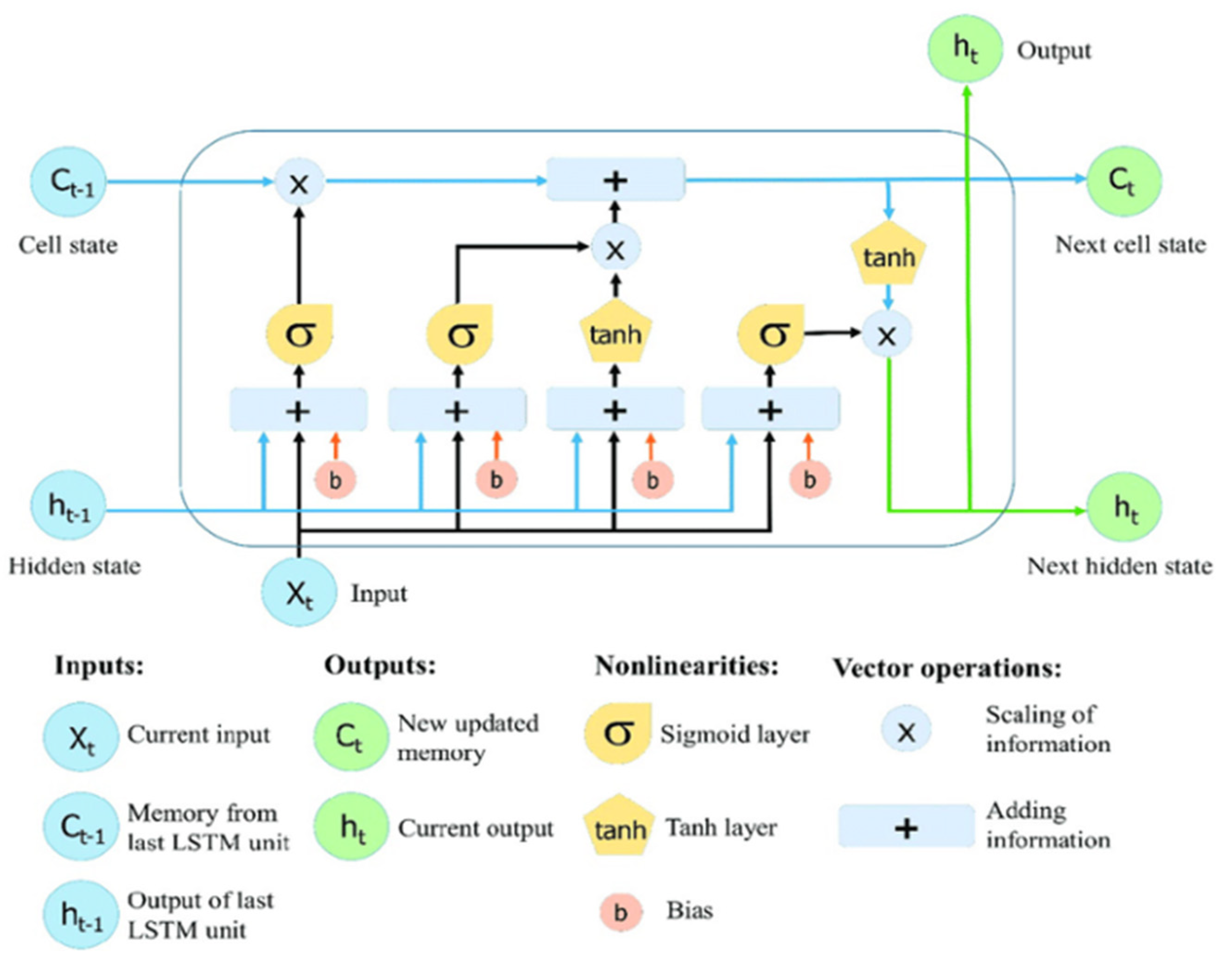
In the literature, there are two varieties of LSTM, the standard LSTM and the LSTM based on the sequence-to-sequence architecture (S2S). Our choice is based on the S2S architecture because of the research undertaken in the framework of electricity consumption prediction. These studies show that the S2S LSTM gives better results than the standard one [19]. Figure 2 shows, in a more pragmatic way, the architecture of an LSTM cell with its inputs and outputs.
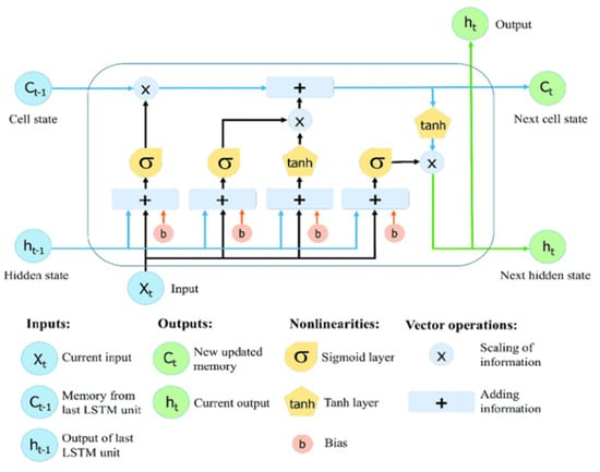
Figure 2.
Architecture of an LSTM cell.
3.2. GRU (Gate Reccurent Unit)
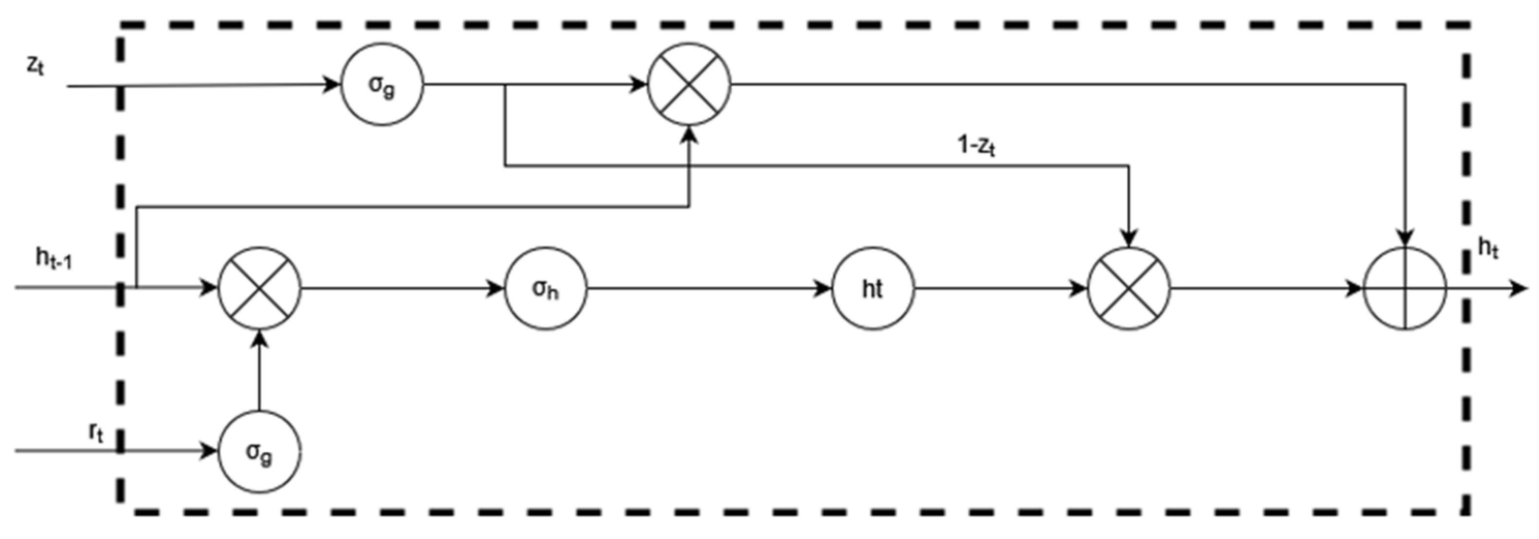
First introduced by Cho et al., GRU is similar to LSTM, but it has fewer gates [20,21]. In addition, it relies only on a hidden state for memory transfer between recurrent units, so there is no separate cell state. In GRU, both the reset gate and the update gate are employed to solve the leakage gradient problem [21], which are two vectors that can manipulate the information in the networks/layers flowing to the desired output [18]. What makes these two gates special is that they can be trained to retain long-term memories, without deleting relevant information that is important for later predictions. Figure 3 shows the structure of a GRU block with inputs and outputs. GRUs are similar to LSTMs but they do not have a cell state vector and they have only two gates, a reset gate r and an update gate z:
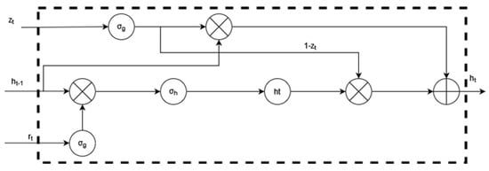
Figure 3.
GRU block architecture.
- -
- the reset gate r determines the amount of information to be forgotten;
- -
- the update gate z defines the amount of information to keep (it works like the forget and input gate of an LSTM).
The reset gate is implemented by Equation (6):
where σg is the logistic sigmoid function, and the index j denotes the jth element of the vector. xt is the input of the neuron at time t and ht−1 indicates the previous hidden state at time t−1. Wr and Ur are the weights of the read matrices and bz is the bias. By analogy, the update gate is expressed by the same equation.
where zt is the gate update function, which is the activation function; Wz and Uz are the weights, xt is the neuron input at time t; ht−1 is the cell state at time t−1; and bz is corresponds to the bias.
Note that the computed reset gate is re-equated to introduce new content into the memory (Equation (8)).
where is the output candidate of the cell state vector, is the activation function, Wz and are the assigned weights, is the neuron’s input at time t, is the memory state at time t−1, and is the bias.
Finally, we need to incorporate the effect of the update gate . This determines the extent to which the new hidden state is simply the old state and the extent to which the new candidate state is used. The update gate can be used for this purpose simply by taking elementwise convex combinations between the two and .
Finally, the current state vector of the cell () is computed to pass the hold information to the next unit. To do this, the update gate () is involved in Equation (9):
3.3. ARIMA
The autoregressive integrated moving average (ARIMA) approach is a time series forecasting method widely used in electrical load prediction [22,23]. Electrical load is the amount of electrical energy consumed by users in a given electrical system. Accurate prediction of electrical loads is essential for the efficient planning and operation of power systems.
This is a generalized autoregressive moving average (ARMA) model, which combines autoregressive (AR) and moving average (MA) processes. In other words, ARIMA (p, d, q) captures the main features of the model: autoregression (AR), integration (I) to make the time series stationary, and a moving average (MA) to take into account the dependencies between the observations and the residual errors [15].
Autoregression (AR) adopts the dependence between an observed value and lagged previous observed values for predictions. In electric load forecasting, this is equivalent to saying that there will be upcoming consumption in the next hour or there may be a peak in consumption in the next hour. The integrated part (I) of the model (d) includes the model terms that incorporate the amount of differentiation to be applied to the time series. The moving average part of the model (q) allows us to define the error of our model as a linear combination of error values observed at previous times [8]. The ARIMA (p,d,q) model using the lag polynomial L is illustrated by Equation (10) [8].
where is the lag operator, represents the autoregressive model parameters, represents the moving average parameters, and are the error terms. Since the parameters of the model have to be defined, we chose the Akaike information criterion for the optimal selection of the parameters.
The Akaike information criterion (AIC) is a commonly used measure for selecting the parameters of an ARIMA model. The AIC criterion is based on the maximization of the likelihood function of the model and takes into account the complexity of the model by adding a penalty for the number of estimated parameters in the model [8,22]. The Akaike criterion is defined as follows:
where k is the number of estimated parameters in the model and is the maximized likelihood function for the model.
The ARIMA model with the smallest AIC is generally considered the best model. This is because the AIC takes into account the goodness of fit of the model (measured by the likelihood) and the complexity of the model (measured by the number of parameters), and thus favors models that provide an adequate fit with a minimal number of parameters.
3.4. Hybrid Models
Hybrid models combining the advantages of ARIMA, LSTM, and GRU models are used in this section to predict electrical peak consumption. In the time series prediction problem, the characteristics of linear and nonlinear models determine that the former can only recognize the linear pattern of the time series, while the latter has the advantage of being able to take advantage of the nonlinear relationship of the time series. The literature shows that many experiments and uses have shown that when using a single series of temporary components, using a single model can be beneficial. However, a single model has limitations when dealing with complex problems. Since the temporal series describing the object of research contains both linear and nonlinear components, it is not possible to use either a single linear or a single nonlinear model [24,25,26]. The equation governing our approach is the following:
where is the original signal, is the linear component, and is the nonlinear component. Figure 4 shows the process modeling flowchart.
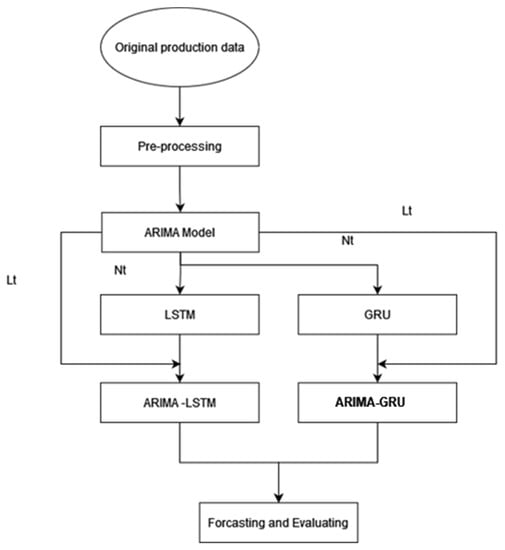
Figure 4.
Hybrid Models flowchart.
4. Methodology
In our work we used data provided by the Electric Company of Benin (CEB) over 4 years (from 2017 to 2021) with a frequency of one hour. These data are missing at certain times, so we used a filter. In the following work we use 80% of the data for training our models and 20% for testing.
The goal of our work is to predict peak consumption, so we go through a series of five models to find the best one for the prediction.
After data acquisition, pre-processing was undertaken in order to eliminate missing data. Once this part was completed, we proceeded to the constitution of a new database of peak consumption. Then we proceeded to the training of our models and to the prediction with the choice of the hyperparameters for a better result. The performance of our models was evaluated by the statistical indicators, as shown in Section 5. A comparison is then made at the end between the different models for each prediction horizon.
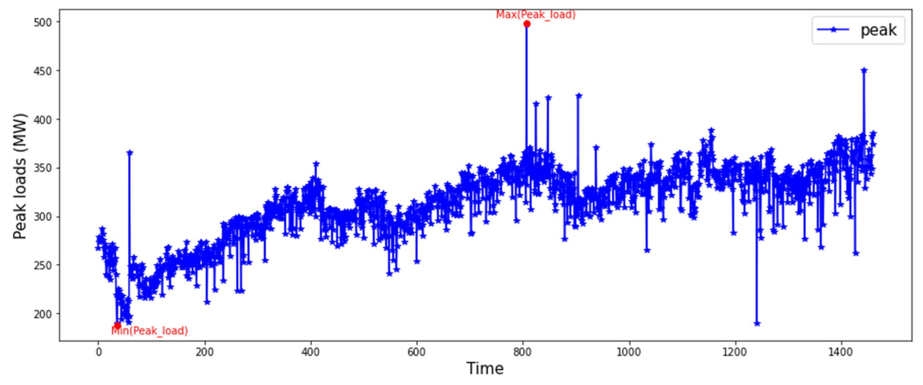
The daily data for our work are shown in Figure 5 and represent the consumption over the four years.

Figure 5.
Peak representation.
GRU and LSTM share an identical deep learning configuration, which has three input layers and one output layer. The number of neurons in the hidden layers was set to 64 for both LSTM and GRU, while a single neuron was designed in the output layer. Before entering the deep learning model, the input data were converted into a matrix with various dimensions depending on the windows chosen. Twenty-four windows were used to determine the most optimal models for prediction. When the deep learning neural networks were compiled, RMSE was specified as the loss function while adaptive moment estimation (Adam) was applied as the optimization algorithm. Compared to ARIMA, we varied the parameters (p, d, q) to determine the optimums that can give a better prediction. This choice was made via the Akaike information criterion. The hybrid models inherit the configurations of the models already used for a better comparison. Thus, the residuals from the ARIMA model are introduced in the neural models. These neural models inherit the basic configurations of the respective single models.
5. Performance Evaluation
In our work, we used RMSE as an indicator of statistical performance to determine the optimal approach for estimation. As noted by several authors, the qualification of a very low root mean square error (RMSE) indicates the performance level of a model as well as the mean absolute percentage error (MAPE) [27,28]. The expressions for calculating the indicators are illustrated by the following equations:
where denotes the ith predicted energy and denotes the ith actual energy. Pao et al. [27] interpreted the results provided by MAPE to judge the accuracy of the prediction approaches used, and found that less than 10% is a very accurate prediction, 10–20% is a good prediction, 20–50% is a reasonable prediction, and more than 50% is an inaccurate prediction.
6. Results and Discussion
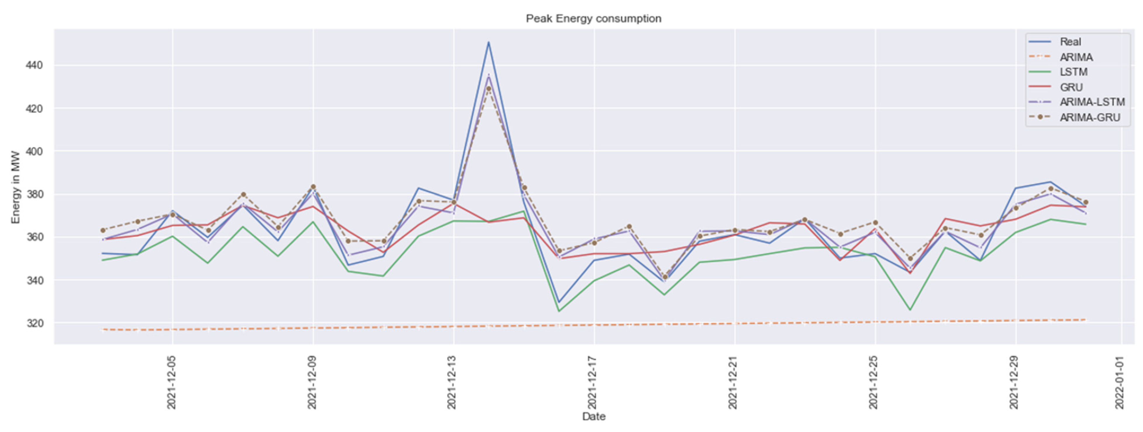
In this part, we predict the consumption peak for the month of December 2021. With the five models, we predicted the data for the last month while optimizing the parameters of our models. For ARIMA, the parameters (p, d, q) are chosen based on the Akaike information criterion. The triplet (2, 1, 2) is chosen as the parameters (p, d, q) for the ARIMA model. As shown in Table 2, we observe that the forecasts made by ARIMA do not align with the actual data. With an RMSE of 49.90 and MAPE of 12.06, they confirm one of the weaknesses of the ARIMA model, namely, its limited ability to accurately predict nonlinear data [29,30]. ARIMA models are based on linear assumptions and are more effective at capturing and forecasting linear patterns in time series data. Thus, this ability to predict linear data will be useful in facilitating the prediction of data by separating the data to be predicted for the hybrid models. In Figure 6, we can observe that the prediction made by the ARIMA model simply follows a straight line.

Table 2.
Statistical indicators.
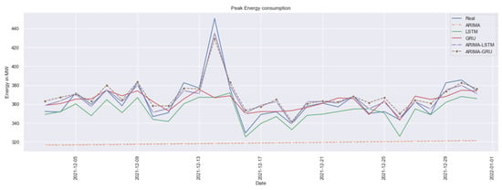
Figure 6.
Peak consumption forecasts.
The neural approaches of deep learning, LSTM, and GRU, give convincing results with respective RMSEs of 18.74 and 18.11, and respective MAPEs of 3.01 and 2.60. These two approaches come closer to the actual results due to their ability to adapt to different types of data. LSTMs and GRUs are more flexible than traditional RNN models. They can handle sequences of varying lengths and adapt to different types of data, whether they are univariate or multivariate time series.
However, the results of the performance indicators for the hybrid approaches are significantly improved. The ARIMA-LSTM approach slightly outperforms the ARIMA-GRU approach with an RMSE of 7.35 compared to 9.60, and in terms of MAPE, ARIMA-LSTM surpasses ARIMA-GRU (1.52% versus 1.56%). This forecasting performance is mainly due to the ARIMA approach. As mentioned earlier, ARIMA is able to better predict the linear part of the input data. One observation is that the GRU approach, which outperformed LSTM in the unimodal prediction, falls behind with the hybrid approach. This reversal is simply explained by the fact that the residual data from the ARIMA model are better predicted by LSTM than GRU. Although there are small differences between the results, both approaches can be used for prediction. As shown in Figure 6, the two approaches almost overlap.
The following figure shows the graph of the predicted and actual consumption. This leads us to better appreciate the impact of the use of hybrid approaches on the prediction. Table 3 shows the values of these peaks of electrical energy consumption. Given this consistency and the accuracy of the hybrid ARIMA-LSTM model, it can be selected as the best model for estimating peak consumption and peak hours.

Table 3.
Predicted data.
7. Conclusions
In this study dedicated to the prediction of peak consumption of electrical energy in Togo, five approaches were studied: ARIMA, LSTM, GRU, and hybrid approaches including ARIMA-LSTM and ARIMA-GRU. The results from the predictions with our models revealed that the hybrid ARIMA-LSTM approach provides better accuracy with an RMSE of 7.35. The results from this work indicate the hybrid approaches are better at predicting peak electrical energy consumption than the single approaches. These results complement the work undertaken in the field, especially in Togo. They will be more useful for the energy distribution company to optimize the external energy purchase policy and to promote the integration of renewable sources in the electrical network as back-up sources. Future work may consider increasing the size of the dataset and re-examine deep learning approaches such as LSTM and GRU.
Author Contributions
Methodology, A.A.P. and A.K.S.; Validation, S.A.A.; Formal analysis, S.A.A.; Resources, S.A.A.; Writing—original draft, A.A.P.; Writing—review & editing, A.K.S.; Supervision, B.B. All authors have read and agreed to the published version of the manuscript.
Funding
The APC was funded by Centre d’Excellence Régionale pour la Maîtrise de l’Electricité.
Data Availability Statement
Restrictions apply to the availability of data. Contact authors for required permissions.
Acknowledgments
We would like to thank the CERME (Centre d’Excellence Régional pour la Maîtrise de l’Electricité) for its support in the research. However, we do not forget the World Bank which allowed this program.
Conflicts of Interest
The authors declare no conflict of interest.
References
- Rallapalli, S.R.; Ghosh, S. Forecasting monthly peak demand of electricity in India—A critique. Energy Policy 2012, 45, 516–520. [Google Scholar] [CrossRef]
- Laouafi, A.; Mordjaoui, M.; Laouafi, F.; Boukelia, T.E. Daily peak electricity demand forecasting based on an adaptive hybrid two-stage methodology. Int. J. Electr. Power Energy Syst. 2016, 77, 136–144. [Google Scholar] [CrossRef]
- Hyndman, R.J.; Fan, S. Density Forecasting for Long-Term Peak Electricity Demand. IEEE Trans. Power Syst. 2010, 25, 1142–1153. [Google Scholar] [CrossRef]
- Pavlicko, M.; Vojteková, M.; Blažeková, O. Forecasting of Electrical Energy Consumption in Slovakia. Mathematics 2022, 10, 577. [Google Scholar] [CrossRef]
- Cao, X.; Dong, S.; Wu, Z.; Jing, Y. A Data-Driven Hybrid Optimization Model for Short-Term Residential Load Forecasting. In Proceedings of the 15th IEEE International Conference on Computer and Information Technology, CIT 2015, Liverpool, UK, 26–28 October 2015; pp. 283–287. [Google Scholar] [CrossRef]
- Fan, G.-F.; Wei, X.; Li, Y.-T.; Hong, W.-C. Forecasting electricity consumption using a novel hybrid model. Sustain. Cities Soc. 2020, 61, 102320. [Google Scholar] [CrossRef]
- Kandananond, K. Forecasting Electricity Demand in Thailand with an Artificial Neural Network Approach. Energies 2011, 4, 1246–1257. [Google Scholar] [CrossRef]
- Guenoupkati, A.; Salami, A.A.; Kodjo, M.K.; Napo, K. Short-Term Electricity Generation Forecasting Using Machine Learning Algorithms: A Case Study of the Benin Electricity Community (C.E.B). TH Wildau Eng. Nat. Sci. Proc. 2021, 1, 189–196. [Google Scholar] [CrossRef]
- Yalcinoz, T.; Eminoglu, U. Short term and medium term power distribution load forecasting by neural networks. Energy Convers. Manag. 2005, 46, 1393–1405. [Google Scholar] [CrossRef]
- Xiong, P.-P.; Dang, Y.-G.; Yao, T.-X.; Wang, Z.-X. Optimal modeling and forecasting of the energy consumption and production in China. Energy 2014, 77, 623–634. [Google Scholar] [CrossRef]
- Manowska, A.; Rybak, A.; Dylong, A.; Pielot, J. Forecasting of Natural Gas Consumption in Poland Based on ARIMA-LSTM Hybrid Model. Energies 2021, 14, 8597. [Google Scholar] [CrossRef]
- Zhou, S.; Song, C.; Zhang, J.; Chang, W.; Hou, W.; Yang, L. A Hybrid Prediction Framework for Water Quality with Integrated W-ARIMA-GRU and LightGBM Methods. Water 2022, 14, 1322. [Google Scholar] [CrossRef]
- Darwazeh, D.; Duquette, J.; Gunay, B.; Wilton, I.; Shillinglaw, S. Review of peak load management strategies in commercial buildings. Sustain. Cities Soc. 2022, 77, 103493. [Google Scholar] [CrossRef]
- Yildiz, B.; Bilbao, J.; Sproul, A. A review and analysis of regression and machine learning models on commercial building electricity load forecasting. Renew. Sustain. Energy Rev. 2017, 73, 1104–1122. [Google Scholar] [CrossRef]
- Siami-Namini, S.; Tavakoli, N.; Namin, A.S. A Comparison of ARIMA and LSTM in Forecasting Time Series. In Proceedings of the 2018 17th IEEE International Conference on Machine Learning and Applications (ICMLA), Orlando, FL, USA, 17–20 December 2018; pp. 1394–1401. [Google Scholar]
- Kolen, J.F.; Kremer, S.C. Gradient Flow in Recurrent Nets: The Difficulty of Learning Long Term. Dependencies 2001, 28, 237–243. [Google Scholar] [CrossRef]
- Kong, W.; Dong, Z.Y.; Jia, Y.; Hill, D.J.; Xu, Y.; Zhang, Y. Short-Term Residential Load Forecasting Based on LSTM Recurrent Neural Network. IEEE Trans. Smart Grid 2019, 10, 841–851. [Google Scholar] [CrossRef]
- Liu, X.; Lin, Z.; Feng, Z. Short-term offshore wind speed forecast by seasonal ARIMA—A comparison against GRU and LSTM. Energy 2021, 227, 120492. [Google Scholar] [CrossRef]
- Marino, D.L.; Amarasinghe, K.; Manic, M. Building energy load forecasting using Deep Neural Networks. In Proceedings of the IECON 2016-42nd Annual Conference of the IEEE Industrial Electronics Society, Florence, Italy, 23–26 October 2016; pp. 7046–7051. [Google Scholar] [CrossRef]
- Cho, K.; Van Merrienboer, B.; Bahdanau, D.; Bengio, Y. On the properties of neural machine translation: Encoder-decoder approaches. arXiv 2014, arXiv:1409.1259. [Google Scholar] [CrossRef]
- Fu, R.; Zhang, Z.; Li, L. Using LSTM and GRU neural network methods for traffic flow prediction. In Proceedings of the 2016 31st Youth Academic Annual Conference of Chinese Association of Automation (YAC), Wuhan, China, 11–13 November 2016; pp. 324–328. [Google Scholar]
- Zhang, Y.; Meng, G. Simulation of an Adaptive Model Based on AIC and BIC ARIMA Predictions Simulation of an Adaptive Model Based on AIC and BIC ARIMA Predictions. J. Phys. Conf. Ser. 2023, 2449, 012027. [Google Scholar] [CrossRef]
- As’ad, M. Finding the Best ARIMA Model to Forecast Daily Peak Electricity Demand. In Proceedings of the Fifth Annual ASEARC Conference—Looking to the future—Programme and Proceedings, University of Wollongong, Wollongong, NSW, Australia, 2–3 February 2012. [Google Scholar]
- Xu, D.; Zhang, Q.; Ding, Y.; Zhang, D. Application of a hybrid ARIMA-LSTM model based on the SPEI for drought forecasting. Environ. Sci. Pollut. Res. 2021, 29, 4128–4144. [Google Scholar] [CrossRef]
- Wang, Z.; Lou, Y. Hydrological time series forecast model based on wavelet de-noising and ARIMA-LSTM. In Proceedings of the 2019 IEEE 3rd Information Technology, Networking, Electronic and Automation Control Conference ITNEC 2019, Chengdu, China, 15–17 March 2019; pp. 1697–1701. [Google Scholar]
- Fan, D.; Sun, H.; Yao, J.; Zhang, K.; Yan, X.; Sun, Z. Well production forecasting based on ARIMA-LSTM model considering manual operations. Energy 2021, 220, 119708. [Google Scholar] [CrossRef]
- Pao, H. Forecasting energy consumption in Taiwan using hybrid nonlinear models. Energy 2009, 34, 1438–1446. [Google Scholar] [CrossRef]
- Debnath, K.B.; Mourshed, M. Forecasting methods in energy planning models. Renew. Sustain. Energy Rev. 2018, 88, 297–325. [Google Scholar] [CrossRef]
- Lee, J.; Cho, Y. National-scale electricity peak load forecasting: Traditional, machine learning, or hybrid model? Energy 2022, 239, 122366. [Google Scholar] [CrossRef]
- Sheng, F.; Jia, L. Short-Term Load Forecasting Based on SARIMAX-LSTM. In Proceedings of the 2020 5th International Conference on Power and Renewable Energy (ICPRE), Shanghai, China, 12–14 September 2020; pp. 90–94. [Google Scholar] [CrossRef]
Disclaimer/Publisher’s Note: The statements, opinions and data contained in all publications are solely those of the individual author(s) and contributor(s) and not of MDPI and/or the editor(s). MDPI and/or the editor(s) disclaim responsibility for any injury to people or property resulting from any ideas, methods, instructions or products referred to in the content. |
© 2023 by the authors. Licensee MDPI, Basel, Switzerland. This article is an open access article distributed under the terms and conditions of the Creative Commons Attribution (CC BY) license (https://creativecommons.org/licenses/by/4.0/).

