Reducing Energy Consumption and CO₂ Emissions in Natural Gas Preheating Stations Using Vortex Tubes

Abstract

This work proposes an innovative method for adjusting the natural gas from the grid to the consumer pipeline requirements in a full-scale pressure reduction station. The use of two counterflow vortex tubes instead of the traditional boiler to preheat the gas before throttling is demonstrated as a powerful alternative. Thus, a reduction of fossil fuel consumption is reached, which amounts to $7.1\%$ less CO${}_2$ emitted. To ensure the optimal configuration, the vortex tube was thoroughly characterized in laboratory facilities using nitrogen as the working fluid. Various operating conditions were tested to determine the most efficient setup. Computational Fluid Dynamics (CFD) simulations were conducted with nitrogen to validate the behavior of the vortex tube. Subsequently, the working fluid was switched to methane to assess the performance differences between the two gases. Finally, the vortex tubes were deployed at a full-scale installation and tested under real consumption demand. The results obtained from this study offer promising insights into the practical implementation of the proposed method for adjusting the natural gas flow, highlighting its potential for reducing fossil fuel consumption and minimizing CO${}_2$ emissions. Further improvements and refinements can be made based on these findings.

1. Introduction

The reduction of fossil fuel consumption is a priority for the industry stimulated by the worldwide policies to reach a climate-neutral scenario in 2050 [1]. In these circumstances, natural gas (NG) suppliers are reconsidering the procedure to accommodate the gas from the distribution grid to the consumption points’ requirements. This adaptation is carried out in a pressure reduction station where the NG is throttled to liberate the excess pressure. However, based on the Joule–Thomson effect, the NG temperature plunges, leading to the unsuitable hydrates formation [2,3]. To avoid this issue, the NG is traditionally preheated before the expansion by means of a boiler, which consumes part of the inlet gas. 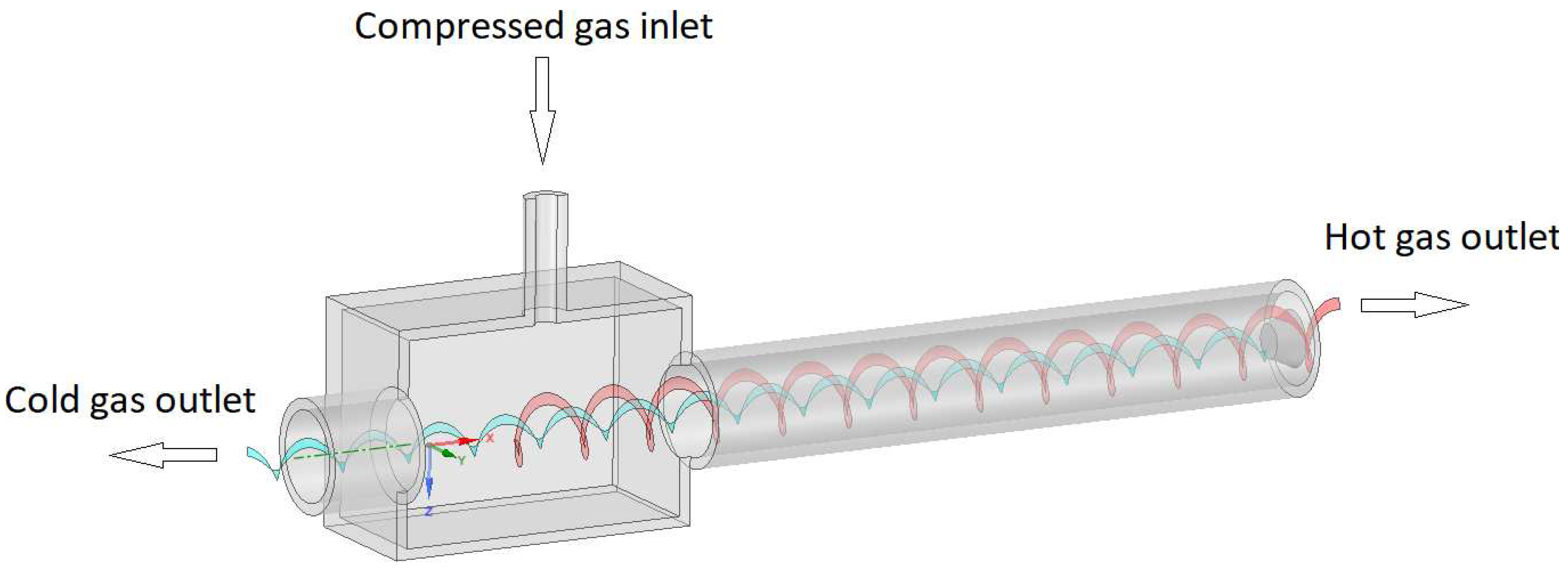Thus, efforts have been focused either on the reduction of the NG boiler consumption [3] or a replacement of this device by, e.g., solar collectors [4], geothermal exchangers [5] or turbo-expanders [6]. In this context, using Ranque–Hilsch vortex tubes (VT) seems a promising alternative since energy input is not required to increase the gas temperature before the expansion. This device is able to generate two separated streams at different temperatures when a compressed gas flow is injected tangentially. The cold stream exits from the central outlet nearby the inlet, and the hot stream is exhausted from the exit at the other side of the tube. Figure 1 represents the flow distribution inside a dual path or counterflow VT. Although single path VT can also be used, some researchers report that this configuration is less efficient than the counterflow one [7]. The main advantage of a VT is its simplicity of design and lack of moving parts. Thus, power input is not required and its maintenance is greatly simplified. Based on these advantages, the VT can be considered an excellent choice for heating and cooling applications, e.g., heating, ventilating and air-conditioned (HVAC), cooling of electronics, gas liquefaction or gas heating [8,9].

The purpose of the present research is to demonstrate the feasibility of substituting the hot water boiler in an actual pressure reduction station with two vortex tubes. The VTs used are specially designed for working with typical pressure gradients found in NG distribution plants and incorporate a novel system to avoid condensation in the cold inlet. This system diverts part of the flow of the hot exit towards the cold one. Due to this novelty, one of the tubes is first tested in laboratory conditions to assess its performance. This is done using nitrogen as a working fluid. The testing is complemented with computational fluid dynamics (CFD) simulations of the same tube using methane. This allows us to estimate the performance of the tube when installed in the actual station. Finally, the field test under real conditions of demand is performed using two tubes to cover higher demands of NG.

The article is divided into four main sections. The introduction briefly reviews previous experimental and CFD studies on VT. Secondly, the methods and materials section details the laboratory setup, design of experiments, and experimental methods for testing the small VT, as well as the methodology for CFD simulation. The results section is divided into laboratory tests, CFD simulations and field tests, in which the obtained results are discussed and compared between them. Finally, the conclusion section summarizes and highlights the obtained results.

1.1. Review of Experimental Works of Vortex Tubes

The VT has been investigated experimentally to assess its performance under varying conditions of geometrical and thermodynamic nature. Thus, in [10,11], the temperature separation as a function of the pressure ratio and flow of natural gas was studied. It was concluded that the VT could be used for liquefying and purifying NG. A more comprehensive research was carried out in [12] encompassing the effect of geometrical parameters, i.e., diameter and length of the main tube, the diameter of the outlet orifice, the shape of the entrance nozzle; and thermo-physical parameters, inlet gas pressure, type of gas, cold gas/mass ratio and moisture of inlet gas. It was found that the efficiency increases with the ratio length to diameter of the tube, while the diameter of the cold outlet presents an optimum value with respect to efficiency and temperature separation. The temperatures’ separation was found to decrease with increasing cold mass fraction (only fractions higher than $0.4$ were studied) and increasing number of nozzles. Instead, they are improved by increasing the pressure ratio.

The conditions inside the tube were investigated in [13]. They measured the pressure, temperature and velocity inside a vortex tube with nitrogen as a working fluid. The inlet condition was changed by rounding the entrance. It was found that this influences the velocities inside the tube and can improve the temperature separation. Similarly, ref. [14] experimentally measured velocities and pressures inside a VT. They studied the influence of geometrical parameters such as inlet nozzles, cold exit, hot exit and length of the tube. The authors found that a forced vortex is formed at the injection point, which gradually transforms into a free vortex towards the hot exit. The free vortex in the central region transfers energy outwards. The same authors carried out an energy analysis of the VT in [14]. Their interpretation is that the temperature drop at the cold exit is due to the pressure gradient, while the temperature rise at the hot exit is due to partial stagnation of the flow. The effect of the number of nozzles and their aspect ratio was studied by [15]. It was also found that increasing number and aspect ratio of nozzle leads to larger mixing zones, which reduces the difference between hot/cold exit temperatures.

An optimization and sensibility analysis were performed in [16], considering the effect of inlet air pressure, hot tube length, hot tube internal diameter, orifice diameter, and nozzle diameter, on hot-outlet air temperature. The Taguchi method was used to optimize the response. It was observed that all parameters studied have a significant impact on hot temperature. Another study on optimization can be found in [17]. They experimentally studied the influence of the number of nozzles, cold orifice diameter and inlet pressure on the cooling performance of a VT. The results were analyzed using the response surface methodology. They show that reducing the number of nozzles increases the cold temperature difference for all pressures studied. Instead, the cold exit diameter presents an optimum value which maximizes that difference. The sensitivity analysis proved that the latter parameter was the most influential of the three analyzed.

Regarding the connection of vortex tubes, [18] studied the performance of two VT in series and in parallel. It was found that the serial setup yields a higher cold temperature difference, while the parallel gives rise to higher hot temperature separation. As with single tubes, it was found that the performance increases with the cold mass fraction and pressure ratio. The present research uses a parallel connection between two tubes in the field tests.

Investigations regarding the use of VT in pressure reduction stations have also been performed recently. Thus, refs. [2,19] assess the feasibility of using a VT to reduce the expense of fossil fuels in the preheating of NG, necessary before distributing the gas to consumers. Both studies conclude that this is an interesting solution allowing us to recover energy and simplifying the station maintenance.

The literature on VT is mounting, ranging from design and operation to basic physics. Some reviews can be found in [7,20,21].

1.2. Review of Simulation of Vortex Tubes

Simulations and models aimed at understanding the physics of vortex tubes have been reviewed by [20]. Ref. [22] employed CFX software to numerically simulate the compressible flow and energy separation of the VT used in Bruun’s experiment [23]. They developed an axisymmetric model and solved the mass, momentum, and energy conservation equations, neglecting the gravity contribution and employing the $\kappa$-$ϵ$ model for turbulence. Ref. [24] conducted CFD simulations for different types and numbers of nozzles, evaluating the swirl, axial and radial velocity components, as well as flow patterns including secondary circulation flow. Optimum cold end diameter and length/diameter ratio were obtained with CFD and validated with experiments. They used the RNG (Renormalization group) $\kappa$-$ϵ$ model for turbulence. Ref. [25] performed a comprehensive 2D axisymmetric CFD model of a real VT and compared it with real experiment measurements. In general, they obtained good agreement between model and experiments. They explored a wide range of cold fractions and temperature separation along it. Ref. [26] made a comparison of different RANS (Reynolds Averaged Navier–Stokes) turbulence models in predicting the temperature separation in VT. As [25], they studied temperature separation against cold fraction, and compared against experimental studies. A 2D axisymmetric model was used. They concluded that standard $\kappa$-$ϵ$ gives the best agreement with experiments in terms of temperature separation. Ref. [27] present a 3D CFD model to study the effect of cold end diameter in temperature separation of VT. They found an optimal cold end diameter for a given VT and claim that CFD is a powerful tool for obtaining optimum parameters in the design of VT. Ref. [28] investigated experimentally and through a 3D CFD model the effect of a conical valve length, as well as the inlet pressure and nozzle intakes. They obtained an optimum cone length for maximum efficiency. Ref. [29] explored the effect of changing the divergence angle of a flared VT and compared it with a straight one, by simulating a 3D CFD model. They applied a periodic boundary condition to reduce the domain to a ${60}^{°}$ sector of the VT.

Regarding the influence of the working fluid on the performance of VT, and specifically with methane or NG there are fewer studies in literature. Ref. [12] performed experiments with three different gases inside a VT, namely oxygen, helium, and air. They found that, among other parameters, the specific heat ratio of gas influenced the temperature separation. Specifically, they found that the higher the specific heat ratio, the higher the cold temperature separation. Ref. [30] found a good correlation between experiments and a mathematical similarity relation with the same three working gases and believed that the better energy separation of helium compared with oxygen and air is due to the much lower molecular weight of helium. Ref. [31] investigated with a 2D compressible CFD model the effect of working gases on energy separation effects. They tested helium, air, nitrogen, oxygen, carbon dioxide, ammonia, and water. They confirmed the results from [12,30] by stating that cold temperature separation was favored by increasing the specific heat capacity ratio and by reducing molecular weight. Ref. [32] performed a 3D CFD simulation, together with an analytical model, comparing the performance of a VT with air and methane as working fluids. They found that both hot and cold temperature separation were lower for methane. In [33], a 3D simulation based on the geometry of [25] is validated and then used to explore the energy distribution inside the tube and the role of the Reynolds stresses. Ref. [34] also performed a 3D CFD simulation of a six nozzle VT, with methane and air as working fluids, arriving at the same conclusion as [32]: methane simulations result in a slightly lower temperature separation for both hot and cold ends.

An important conclusion from the CFD simulation survey is that a 2D axisymmetric model using a compressible fluid and the $\kappa$-$ϵ$ model for turbulence is adequate to reproduce the separation of temperatures at the exit of the VT and the pressure ratio. For its balance of simplicity and accuracy, this will be the simulation setup of choice for this work.

2. Materials and Methods

This section explains in detail the materials and procedures followed to perform the experimental tests and simulation studies. The results are revealed in the next section.

2.1. Laboratory Tests

The experimental tests were done with a VT whose nominal flow is 74 Nm${}^3$/h (GR1, 600 mm in length and 31 mm in diameter). A schematic of the experimental setup is shown in Figure 2. In the field test, an additional VT with double nominal flow (GR2, 710 mm in length and 40 mm in diameter) will be used. This was not tested in the laboratory due to the difficulty to achieve enough gas supply. However, both VTs have the same design and are expected to behave analogously under the right conditions of pressure ratio and flow rate. The objectives of the tests were:

• Verify that the flow division corresponds to the design, i.e., $60\%$ cold.
• Verify the temperature increase in the hot side and the temperature decrease in the cold side.
• Study the dependence between the flow rate and the pressure ratio $P_{in}/P_{out}$.
• Study the performance of the vortex tube at different ratios, to check the right operation of the system under different conditions.

The tests were carried out under these general conditions:

• The working gas was nitrogen.
• The working pressure in the inlet manifold ranged from 3 to 9 barg.
• The pressure in the outlet manifold (of the testing installation) was set to 1 barg.
• The estimated stabilization time of the installation was 2 min. An additional 8 min were added for data collection and verification. In two cases, due to nitrogen supply problems, the tests were shortened by two minutes.

The inlet pressure range is limited from below by the minimum pressure ratio required by the VT to achieve a good separation of hot/cold streams. According to the manufacturer, this ratio needs to be higher than 2. The maximum pressure is limited by the supply system, which consists of a rack of pressurized cylinders. The pressure at the outlet is chosen to be similar to that found in the actual plant in which field tests will be performed. The duration of each test was chosen considering the stabilization time of the VT and the availability of gas at the required pressure.

The experimental tests performed are summarized in

Table 1. Experiments carried out in the laboratory.

Test	${\mathit{P}}_{\mathit{in}}$ (barg)	${\mathit{P}}_{\mathit{out}}$ (barg)	Duration (min)
1	3	1	10
2	3.5	1	10
3	4	1	10
4	4.5	1	8
5	5	1	8
6	6.5	1	8
7	9	1	8

. The time recorded is the total time, i.e., including the stabilization of the VT.

During a test, the pressure and temperature can be measured by a PLC (Programmable Logic Controller) system, while the flow has to be obtained as the difference between the initial and final count in a flow meter. In

Table 2. Instrumentation used in the laboratory and field tests.

Measure	Instrument	Model	Uncertainty
Gas flow	Rotary gas meter	2xG65 DN 50	0.5–1%
Gas flow	Rotary gas meter	2xG65 DN 80	0.5–1%
Temperature	Thermocouple	NIVELCO Thermocount TN	Class A (EN 60751)
Pressure	Pressure transducer	Gems Sensor 865	0.25 ±% FS

, we list the instruments used in the laboratory and field tests. The measurements are annotated at a frequency of 1 min. For analysis, the average of the measured values during the test and the final value reached have been used.

2.2. CFD Simulations

The purpose of the simulations is to obtain a prediction of the effect of switching the working gas of the VT from nitrogen to methane. The first step is to develop a model that reproduces the observed behavior with nitrogen, using the experimental tests as a guide. Afterwards, the nitrogen is replaced by methane.

Since the detailed geometry of the VT is not known, there is no advantage in modeling an inaccurate 3D model, given that, as the literature consulted shows, a 2D axisymmetric model can replicate the behavior of a real VT. For that reason, a 2D axisymmetric model was developed. The gas inlet has been modeled as an annular inlet, following the approach of [25]. The cold and hot outlets are modeled as cylinders, with the hot side partially covered by a cylindrical valve. Figure 3 shows a recreation of the resulting 3D VT, and a detail of the hot outlet valve.

The flow of gas enters the tube with a swirl momentum due to the angle $\theta$. This parameter recreates the orientation of nozzles in real tubes. The swirl is a result of the radial and tangential components of the velocity, while the axial component is set to zero. The cold and hot outlets have been lengthened to allow a developed outlet flow profile, which helps to stabilize the numerical solution. The resulting 2D geometry is depicted in Figure 4, though only half of it had to be simulated thanks to symmetry respect to the axis. “L” stands for length, “D” for diameter, and subscripts “t”, “h”, “c”, “i”, “hv” stand for “Vortex tube”, “hot outlet”, “cold outlet”, “inlet” and “hot valve”, respectively. The dimensions of GR1 in the simulation are gathered in

Table 3. Relevant fixed geometric dimensions of simulated VT.

${\mathit{L}}_{\mathit{t}}$ (mm)	${\mathit{L}}_{\mathit{c}}$ (mm)	${\mathit{L}}_{\mathit{h}}$ (mm)	${\mathit{D}}_{\mathit{t}}$ (mm)	${\mathit{D}}_{\mathit{c}}$ (mm)	${\mathit{L}}_{\mathit{t}}/{\mathit{D}}_{\mathit{t}}$
600	60	60	31	12.7	19.35

.

Since the detailed geometry is unknown, the procedure to replicate the tube is the following:

(1)

Develop a 2D model with three free geometric parameters. These parameters are:

(a)

Size of the hot valve ($L_{hv}$ in Figure 4).

(b)

Size of the inlet ($L_i$ in Figure 4).

(c)

Angle of inclination of the inlet ($\theta$ in Figure 5).

(2)

Perform a parametric sweep of those parameters by CFD to obtain the values that replicate the results provided by the manufacturer, in terms of temperature separation and pressure ratio.

(3)

Once the right values for the parameters are obtained, perform simulations to replicate the laboratory tests.

Before the parametric sweep, it is necessary to ensure that the used mesh is good enough to trust its results. For that purpose, a mesh sensitivity analysis was performed. Since the above-mentioned geometric parameters are unknown, generic values were used, $L_{hv}=75$ mm, $L_i=2.5$ mm, $\theta =5.5^{°}$. As the monitored variables to assess the convergence of the mesh, temperature separation in cold and hot outlets were selected, since they are the most important performance indicators of the VT. The results for the analysis are shown graphically in Figure 6. In

Table 4. Mesh sensitivity analysis metrics. Relative variation in temperatures’ separation between successive refinements of the mesh.

Elements	$\mathbf{\Delta }{\mathit{T}}_{\mathit{hot}}$$(\%)$	$\mathbf{\Delta }{\mathit{T}}_{\mathit{cold}}$$(\%)$
31,488	-	-
46,686	2.70	2.43
65,609	1.07	0.97
87,279	0.60	0.55
95,064	0.12	0.11
108,106	0.23	0.21
117,033	0.10	0.09
140,835	0.28	0.27
165,193	0.24	0.23
193,352	0.37	0.36

, the relative differences between the results of a mesh and its previous one are shown. Given the low variation for values higher than ∼90 k cells, the selected mesh is the one with 95,064 elements. The mesh comprises quadrilateral cells with a few triangular cells. The maximum cell size is $0.5$ mm while at the inlet it decreased to $0.073$ mm, and at the exits it is $0.15$ mm in the hot and $0.122$ mm in the cold. The average aspect ratio is very close to 1 indicating that the mesh has a high quality.

Both nitrogen and methane are considered as compressible ideal gases, with temperature-dependent thermophysical properties. Navier–Stokes equations for a 2D axisymmetric problem with swirl were solved, along with energy equation and the two equations of the turbulence model. Turbulence has been modeled through the $\kappa$-$ϵ$ standard model, as suggested by many other researchers, such as [25,26,27,28]. An $y+$ insensitive near-wall modeling was employed, the so-called Menter–Lechner formulation. The viscous heating option was enabled since, for compressible flows, this factor can be important. According to [35], this effect is important when the Brinkman number $Br=\frac{\mu U_e^2}{k\mathsf{\Delta }T}$ approaches or exceeds the unit. In the performed simulations, a value of $Br$∼3 was found, which justifies the use of the viscous heating effect.

For solving the set of equations, a coupled pressure–velocity coupling scheme was used, with a pseudo-time method, using the conservative length scale method, and a second order upwind scheme was used for all the equation discretizations. Furthermore, the equations were solved using a double-precision solver. Convergence was assessed by monitoring the residuals, the average temperature at both outlets, as well as the pressure at the inlet and outlets. When the temperature and pressure showed steady conditions, the simulation was considered to be converged.

Regarding the boundary conditions, walls are considered adiabatic and non-slipping, since they are well insulated from the environment; the mass flow inlet is fixed, as well as the outlets, for ensuring the cold ratio of $60\%$ provided by the manufacturer as an operating condition. These boundary conditions, along with their numerical values, are collected in

Table 5. Applied boundary conditions in CFD simulations.

Working Gas	Wall Treatment	Inlet Temperature ($°$C)	Inlet Mass Flow (Nm${}^3$/h)	Cold Outlet Mass Flow (Nm${}^3$/h)	Hot Outlet Mass Flow (Nm${}^3$/h)
Nitrogen	Adiabatic	$-11$	73	$43.8$	$29.2$
Methane	Adiabatic	$-11$	73	$43.8$	$29.2$

. For the inlet turbulent boundary conditions, the hydraulic diameter and a turbulence intensity of $5\%$ were set.

With the above boundary conditions, an optimization study was performed to find the three values of the geometric parameters, which result in the pressure ratio and temperature separation found in the laboratory for nitrogen gas, reported in the results section.

After replicating the experiments with nitrogen, the working fluid is changed to methane in the simulations to obtain predictions of temperature separation when VT is used in the pilot natural gas plant. The same boundary conditions were used (Table 5; note that, while normalized volumetric flow is the same, mass flow changes to adapt to the change in density between nitrogen and methane).

3. Results and Discussion

3.1. Laboratory Tests

The results obtained are presented: (i) by averaging the temperature jumps during the duration of the experiment (average separation) and (ii) the separation at the end of the test, without averaging (final separation).

The temperature separations are reported in an absolute value. That is, the hot temperature separation represents the increment measured in the hot exit with respect to the inlet. Similarly, the cold separation is the decrement measured in the cold exit respect to the inlet.

We have estimated the uncertainty in our measurements by analyzing the results of repeated experiments under the same conditions. The relative errors are in the range 5–12%. However, uncertainties do not affect equally all experiments. Those carried out with large pressure ratio and large flow rate show less uncertainty than experiments with small pressure ratio and flow rate. As can be seen in the following sections, when the operating conditions are close to their lower end, the behavior of the vortex is not stable and exit temperatures fluctuate. The standard deviations expressed as a percentage with respect to the average lie in a similar range to the relative error and show the same trend.

3.1.1. Temperature Separation Measurements

Figure 7a shows the temperature separation in GR1 as a function of the pressure ratio. On the hot side, there is a monotonic increase in temperature, which reaches around 45 $°$C at $P_{in}/P_{out}=4.9$. On the cold side, there is no clear trend. All temperature drops are between 0 $°$C and 10 $°$C. This is due to the by-pass implemented by the vortex manufacturer to bring part of the flow from the hot outlet to the cold outlet to avoid condensation.

Figure 7b shows the same information as a function of the gas flow rate. The gas mass flow rate increases linearly with the pressure ratio (see Figure 8); therefore, the temperature separation follows the same trend as with the pressure ratio.

The results of this section confirm that the temperature separation increases with the pressure ratio. Compared with traditional designs that do not include a by-pass from the hot exit to the cold one, the hot temperatures reached are around 10 $°$C lower. On the other side, the cold temperatures are around zero instead of below, which can be advantageous when mixing the two currents in the exit collector. The cold exit temperature will rise in the field test by means of an atmospheric exchanger. An important observation is that the VT needs to reach its nominal flow rate to start to increase the temperature jump. This can be checked in Figure 7b, where the hot temperature rise decays slightly for flow rates below ≈75 Nm${}^3$/h.

3.1.2. Thermodynamic Analysis

In this section, the VT is analyzed in terms of its efficiency. To account for the energy losses we compute the enthalpy at the inlet of the tube, $H_{in}$, and the enthalpies at the cold and hot exits, $H_{hot}$ and $H_{cold}$, reported in

Table 6. Summary of thermodynamic and efficiency analysis for GR1. Enthalpies are given in W.

Test	${\mathit{P}}_{\mathit{in}}/{\mathit{P}}_{\mathit{out}}$	${\mathit{H}}_{\mathit{in}}$	${\mathit{H}}_{\mathit{cold}}$	${\mathit{H}}_{\mathit{hot}}$	RD (%)	${\mathit{\eta }}_{\mathit{isen}}(\%)$	$\mathbf{\Delta }\mathit{S}(\%)$
1	2.12	7343.71	2815.81	4806.55	−3.8	6.03	75.2
2	2.29	8555.30	3419.48	5317.47	−2.1	5.34	72.8
3	2.61	9807.77	3809.09	6016.02	−0.2	15.22	76.7
4	2.81	10,527.80	4286.82	6548.19	−2.9	1.95	78.4
5	3.02	11,676.13	4741.60	7270.27	−2.9	7.91	79.0
6	3.77	14,860.98	5826.57	9482.10	−3.0	6.10	81.4
7	4.88	19,309.05	7423.37	12,564.07	−3.5	7.43	82.3

. The difference is given as a relative difference (RD) respect to the inlet:

$$RD=100\times \frac{H_{in}-H_{cold}-H_{hot}}{H_{in}}.$$

(1)

The enthalpies increase linearly with the pressure ratio (or the flow rate); however, there is no systematic trend in the relative difference. These differences are consistently close to $3\%$ for most experiments, which is a satisfactorily low value. It must be considered that these losses account for the effect of the pipes, given that the measurements cannot be made right at the inlets/outlets of the tube. So, the results can be improved using insulation in the pipes.

The production of entropy ($\mathsf{\Delta }S$) is given as the relative increase respect to the inlet. Entropy increases notably as it always does in gas expansion, but in this case the effect is enhanced due to the high pressures in the inlet. Correspondingly, the production of entropy increases with the pressure ratio.

To compare these results with those of other groups, we compute the isentropic efficiency, ${\eta }_{isen}$, as defined in [36]. This is the ratio of enthalpy change of the inlet and cold outlet to the enthalpy change of the isentropic expansion of the process. Assuming that the gas is ideal, one obtains

$${\eta }_{isen}=\frac{T_{inlet}-T_{cold}}{T_{inlet}\left(1-{\left(P_{out}/P_{in}\right)}^{\frac{\gamma -1}{\gamma }}\right)}$$

(2)

where $\gamma =C_p/C_v$ is the ratio of heat capacities of the gas. The results are given in Table 6 as a percentage. They are close to $6\%$ for most cases without any systematic trend. The efficiency reported in [36] changes with the cold mass fraction, showing a maximum between 60–70%. For a cold mass fraction of $60\%$, the design value for GR1, their efficiency is ≈12%, indicating that the tube used in this research is less efficient.

From this analysis, it can be concluded that the vortex tube presents fairly low losses of energy, and an efficiency in the range of similar tubes studied in the literature, albeit somewhat lower. The losses in energy could be compensated by using insulation in the connecting pipes.

3.2. CFD Simulations

The results from the parametric study, in which inlet length, inlet angle and hot valve length were swept to reproduce laboratory tests with nitrogen gas (see

Table 7. Mean values of temperature separation from experiments with nitrogen gas.

Hot Temperature Separation ($°$C)	Cold Temperature Separation ($°$C)	Pressure Ratio
29	4.5	2.1

), are gathered in

Table 8. Obtained values from CFD replication of experiments with nitrogen gas, and comparison with experimental values.

Hot Temp. Separation ($°$C)		Cold Temp. Separation ($°$C)		Pressure Ratio
Value	Deviation $(\%)$	Value	Deviation $(\%)$	Value	Deviation $\mathbf{(}\mathbf{\%}\mathbf{)}$
25.8	−11.0	4.7	4.4	1.86	−11.4

. The internal system for avoiding condensation in the cold stream needs to be accounted for in the CFD simulations. This was done by substituting the complex real system by its thermal effect on cold outlet walls. Thus, a positive heat flux boundary condition has been set, so the stream in the cold side is heated up to the temperature separation obtained in the experiments. Since the real heat flux to the cold stream is not known, it is added as another optimization parameter. The criterion used to decide which is the best set of parameters is to minimize the relative sum of the absolute differences between calculated and target temperatures (cold and hot sides). The values of the parameters were $L_i=2.2$ mm, $\theta ={80}^{°}$, $L_{hv}=6$ mm and the heat input was 212 W.

The maximum difference between target and calculated values is $11.4\%$. The low pressure ratio is due to the point of measurement, which is different in simulations and experiments. In the former, the pressure ratio is computed between inlet and cold outlet; in the real vortex tubes, the pressure is measured before gas enters the nozzles. It is reasonable to think that a significant pressure gradient takes place between nozzles inlet and tube inlet.

A characteristic temperature profile inside the VT is shown in Figure 9a. Taking advantage of the capabilities of the simulation, we show the result of removing the heating system (Figure 9b), i.e., the result that would be obtained with a conventional VT tube, for comparison. The effect of the heating device can be seen in the cold outlet, more marked in the corners. The cold plume (up to yellow color) penetrates slightly more into the tube than in the non-heated case. But beyond this point, no appreciable differences in the profile are discernible. This result is interesting because it shows that the new design (diverting part of the hot flow to the cold side) does not significantly alter the conditions inside the tube.

It is not possible to validate the inner tube temperature distribution, since there are no measurements of it at any point. Nevertheless, the obtained profiles perfectly match in shape and qualitative features with all the consulted literature.

For the simulations with methane as a working gas, the results, along with the relative differences with respect to the nitrogen simulations, are collected in

Table 9. Obtained results from CFD simulations with methane, and comparison with nitrogen simulations.

Hot Temp. Separation ($°$C)		Cold Temp. Separation ($°$C)		Pressure Ratio
Value	Diff. $(\%)$	Value	Diff. $(\%)$	Value	Diff. $(\%)$
16.6	−34.9	0.3	−93.6	1.57	−15.6

.

All the relevant variables take lower values than those from nitrogen. As mentioned in the introduction, reference [32] also obtained a lower value of temperature separation when comparing air (mostly nitrogen) and methane. The hot temperature separation is a $30\%$ lower than that obtained without heating, but cold temperature separation is very near to zero, significantly differing from the 4 $°$C obtained with nitrogen. The pressure ratio to obtain the 60–40 (cold-hot) fraction ratios and with the operating mass flow is about 15–20% lower than those needed by nitrogen.

The temperature profiles inside the tube are depicted in Figure 10, along with a profile of a non-heated case for comparison. The temperature gradients are smoother in the case of methane compared to nitrogen. However, the profiles of both working gases share similar qualitative features. The region with the lowest temperatures is the same in both cases, in a half oval-shaped region around could outlet. And for both gases, the differences between the non-heated and the heated cases are very small and confined to the region near the cold outlet.

4. Field Tests

The last step of the research was to implement the studied vortex tubes in a real environment, under typical natural gas regasification station conditions. The station where the two VT (see Section 2.1) have been tested (see schematic in Figure 11 top) has a single liquefied natural gas (LNG) tank and a series of atmospheric heat exchangers, where the regasification occurs. Finally, the gas is heated in a boiler, odorized and injected into the grid. The purpose of the vortex tubes is to substitute the gas heating system, thus avoiding water-heating costs and maintenance, and reducing the pressure of the re-gasified natural gas to that of distribution and supply. Hence, the vortex tubes are placed (Figure 11 bottom) after the first set of atmospheric heat exchangers—this way they can receive the pre-heated gas (at near atmospheric temperatures) and separate it in the hot and cold flows. The hot flow goes directly to the outlet manifold, while the cold one passes through another atmospheric heat exchanger, with the purpose of raising its temperature and thus obtaining a greater final temperature. Then, the cold flow becomes mixed with the hot one in the outlet manifold. Finally, the gas is odorized and injected into the grid.

The gas inlet pressure here was 4 barg, which is the outlet pressure of the LNG tank, and the outlet pressure is around 1 barg. Actually, the outlet pressure varies slightly depending on the demand of gas from the grid. The gas pipes and the atmospheric heat exchangers are both exposed to the ambient temperature, which during the tests ranged from 0 $°$C to 15 $°$C. The main objective of these tests was to assess whether the vortex tubes can replace the current heating system and compare their performance with the observations made in the laboratory and the simulations.

The results of the above operations under various VT flow and pressure parameters during over a month (34 days) period are presented in

Table 10. Main data obtained during the field tests. Temperatures are measured in $°$C, flow rates in Nm${}^3$/h, and the hot fraction of flow rate is a % of the total.

Quantity	Period 1	Period 2	Period 3	Period 4	Period 5	Period 6	Period 7
Global
$T_{out}-T_{in}$	3.1	3.9	4.16	3.22	3.3	3.02	3.75
Flow rate	89.9	132.3	123.80	132.4	172.3	126.2	132.2
$P_{in}/P_{out}$	1.84	2.04	2.09	2.03	1.95	2	1.86
GR1
$\mathsf{\Delta }{T}_{hot}$	11.3	13.8	13.60	6.9	6.2	6.3	7.3
$\mathsf{\Delta }{T}_{cold}$	8.9	10.9	11.00	10.70	10.2	10.5	12
Flow rate	64.1	75.1	74.80	79.10	67.7	70.4	76.2
Hot fraction	39.9	39.6	39.20	57.80	57	54.5	58.8
$P_{in}/P_{out}$	1.83	2.05	2.02	2.02	1.95	2	2.14
GR2
$\mathsf{\Delta }{T}_{hot}$	9.1	11.2	11.20	11.50	10.01	11.4	11.8
$\mathsf{\Delta }{T}_{cold}$	8.3	9.6	9.60	9.50	8.4	10	10
Flow rate	73.9	112.8	119.60	128.70	136.9	130.80	126.5
Hot fraction	53.9	44	42.70	39.00	35	40	38.8
$P_{in}/P_{out}$	1.82	2.03	2.36	2.38	1.82	2	2

. Note that the first 3 rows of the Table 10 correspond to performance of the whole facility, while the other 10 rows are divided into two blocks of five for each vortex tube.

The presented data are averaged over time. Due to the dynamic changes in the demand of gas, over a day there are periods in which only one tube works, or both or none. In practice, however, the case in which both VT are required at the same time never arose. For this reason, the flows shown do not add up to give the total of the facility. Actually, one can deduce that most of the time it is the bigger tube (GR2) that is working. Due to the average, the peak values reached in the temperatures are somewhat higher than those reported in the Table 10, but those peaks are short-lived and, as such, do not represent any long-term behavior.

Period 1 and Period 2 were dedicated to the fine tuning of the facility and the values reported are not representative. In Period 3, an adequate adjustment of the elements of the facility was reached. Effectively, the pressure ratio is above 2 for both tubes, both have a hot fraction of $40\%$ and the flow is very close to the nominal. During this period, it is achieved the maximum average gain in temperature, $4.16$$°$C. During Period 4, unfortunately, an error in the manipulation of the hot exit valve of GR1 caused an increase in this fraction, up to $57\%$. This immediately causes a drop in the performance of the tube, especially noticeable in the hot exit temperature. This, in turn, produces a decrease in the overall gain of temperature of 1 $°$C. Instead, GR2 continues to perform well in periods 4 to 7, even though the pressure ratio is barely 2, i.e., in the limit of validity by design.

Regarding the maximum temperature differences (see Figure 12), it has been observed that the largest ones are registered when the inlet flow rate is close to the nominal flow. This is especially noteworthy in vortex GR1, where the maximum temperature differences are the highest at 73 Nm${}^3$/h, reaching the largest hot temperature difference at $15.35$ $°$C, and the largest low temperature difference at $14.76$ $°$C, with pressure ratios always above 2. It is expected, according to laboratory results, that when operating with higher pressure ratios larger temperature differences should be reached. In the case of vortex GR2, the largest temperature differences are $13.86$ $°$C for the hot side and $12.14$ $°$C for the cold side, for an inlet flow of $145.38$ Nm${}^3$/h and a pressure ratio above 2. A larger temperature difference should also be expected in this case for higher pressure ratios, as for the GR1 case. Additionally, it is also worth noting that the vortex should always be operated with pressure ratios ($P_{in}/P_{out}$) above 2, as this also determines the amount of energy that can be transferred to the gas in the form of heat. The higher this pressure ratio is, the larger temperature differences should be observed. Summarizing, the largest temperature differences should be expected when the inlet flow rate is close to the nominal flow and the pressure ratio is as high as possible.

These results are different in comparison with those obtained in the laboratory, where the mean temperature differences are around 25 $°$C (hot side) and 5 $°$C (cold side). The reduction in temperature gain was predicted by our CFD simulations (see Table 9). Some authors [31] have reported the following observations regarding the temperature separation:

• It increases upon decreasing the molecular weight of the gas.
• It increases upon increasing the $C_p/C_v$ ratio of the gas.

When the working gas is switched from nitrogen to natural gas (${\mathrm{CH}}_4$), the molecular weight is decreased (from $28.02$ to $16.04$) and the $C_p/C_v$ ratio is decreased (from $1.4$ to $1.299$ at 300 K and 1 atmosphere). Clearly, the matter of the dependence of the exit temperatures with respect to the properties of the working gas deserves more investigation.

It can also be noted that vortex GR2 raises the total temperature differences slightly less than GR1. This is due to the average flow being below nominal and the pressure ratio just above 2. These two parameters are key to the optimum performance of the tubes. Should the conditions in the plant allow for a higher inlet pressure, both parameters would increase, thus allowing it to reach greater gas temperature increments, as was observed in the laboratory tests.

As for the whole facility, the maximum obtained temperature differences are shown in Figure 13, again showing a clear dependence on the pressure ratio and flow rate. In this case, the final temperatures are lower than those observed in the laboratory due to the reasons explained above. These temperatures are around 7 $°$C at their best, with mean values of around $5.5$ $°$C. Thanks to these data, the dependence on the pressure ratio and flow ratio can also be confirmed.

4.1. Thermodynamic Analysis

The enthalpies at the inlets and outlets of each vortex and for the whole vortex facility are reported in

Table 11. Summary of thermodynamic and efficiency analysis for field tests. Enthalpies are given in W, the relative difference, isentropic efficiency ${\eta }_{isen}$ and relative entropy increase $\mathsf{\Delta }S$ in %.

Quantity	Period 1	Period 2	Period 3	Period 4	Period 5	Period 6	Period 7
GR1
$H_{in}$	7577.7	9755.5	9510.2	8428.4	7061.8	5715.7	6897.6
$H_{hot}$	3050.9	3941.9	5607.4	4915.9	4055.9	3136.0	4087.0
$H_{cold}$	4522.7	5811.9	3957.9	3513.1	3004.8	2572.4	2806.7
RD	0.1	0.0	−0.6	0.0	0.0	0.1	0.1
${\eta }_{isen}$	19.8	20.4	20.9	20.1	21.5	21.3	22.3
$\mathsf{\Delta }S$	40.9	45.0	44.1	44.0	43.5	41.2	45.8
GR2
$H_{in}$	1110.6	3615.4	3963.4	7783.3	10,492.1	12,143.0	13,387.2
$H_{hot}$	492.8	1611.4	1567.1	3083.2	3725.7	5067.6	5314.9
$H_{cold}$	616.4	2002.1	2389.6	4691.7	6745.2	7066.1	8056.4
RD	0.1	0.1	0.2	0.1	0.2	0.1	0.1
${\eta }_{isen}$	19.2	19.2	19.1	18.3	19.4	20.1	20.1
$\mathsf{\Delta }S$	40.5	44.9	46.8	43.9	43.5	40.9	44.5
Global
$H_{in}$	8688.3	13,370.9	13,473.6	16,211.8	17,556.8	14,965.1	20,284.8
$H_{out}$	8714.1	13,425.3	13,530.2	16,280.1	17,624.6	15,050.1	20,375.8
RD	0.30	0.41	0.42	0.42	0.39	0.57	0.45
$\mathsf{\Delta }S$	51.7	55.8	44.2	43.4	55.9	40.4	44.9

. The relative differences are computed as $RD=100\times (H_{in}-H_{cold}-H_{hot})/H_{in}$ for the VTs and as $RD=100\times (H_{in}-H_{out})/H_{in}$ for the whole vortex facility. The mismatch in enthalpy between inlets and outlets is very small, almost negligible. For the field tests, the pipes of the facility were insulated, which explains the reduction in losses with respect to the laboratory results. The thermal efficiency (${\eta }_{isen}$) of each vortex improves greatly compared to the laboratory observations. This improvement has two sources. For one side, the insulation of the pipes since, as explained before, the probes cannot be placed right at the inlet/outlets of the VTs. On the other side, the definition of ${\eta }_{isen}$ depends on the gas through the ratio of heat capacities $\gamma$. Since the laboratory and field tests have been made with different gases, this quantity is not directly comparable.

The results for the whole facility are analogous, showing negligible losses in energy. Although the figures are very small, it is worth noting that the losses for the whole facility are systematically larger than those for each VT. This is not only consistent, but strongly indicates that the losses come from the connecting pipes rather than from the tubes.

The relative entropy production is in the range 40–50% for both VTs and for the whole facility, with some values above 50% in the latter. These values are lower than those measured in the laboratory at similar pressure ratio, indicating that the latter were affected by heat losses that have been avoided in the field thanks to the insulation.

Note that the isentropic efficiency is not computed for the whole facility because in this case there is no cold exit, as required by the definition.

4.2. Reduction of Emissions

From the results of period 3 we estimated the non-emitted CO${}_2$. This period was chosen because the VT worked with the best adjustment of all elements of the facility. The calculation was made as follows:

• The energy gained by the gas between the inlets of the VT and odorization system inlet was calculated by using the following equation for the whole period, with i representing each period sample, ${\dot{m}}_{VT}$ the mass flow rate of gas through VT, and $C_{p,{\mathrm{CH}}_4}$ the specific heat of natural gas:

  $$\dot{Q}=\sum _{i=1}^{end-of-period}\mathsf{\Delta }{T}_{in-out}{\dot{m}}_{VT}·C_{p,{\mathrm{CH}}_4}$$

  (3)
• The needed CH${}_4$ for heating up the gas is obtained assuming that it is burned in a boiler with an efficiency of $\eta =0.4$, applying the equation below, with LHV${}_{{\mathrm{CH}}_4}$ as the low heating value of natural gas:

  $${\dot{m}}_{C{H}_4,combustion}=\frac{\dot{Q}}{LH{V}_{{\mathrm{CH}}_4}·\eta }$$

  (4)
• The calculated CH${}_4$ mass is transformed into equivalent CO${}_2$ by using the molecular weight ratio of both gases.
• The CO${}_2$ mass from the previous step is divided by the total CO${}_2$ emitted before the installation of VT (equivalent to the 0.5% of natural gas flow, according to the facilities’ owner, calculated as in the previous steps, but considering the total flow of natural gas through the installation), therefore obtaining the relative value as follows:

  $${\mathrm{CO}}_{2reduction}[\%]=\frac{{\dot{m}}_{{\mathrm{CO}}_2,from-avoided-combust}}{{\dot{m}}_{{\mathrm{CO}}_2,from-NG-combust}}·100=7.07\%$$

  (5)

Considering that the test could not be made during the coldest months of the year, the final reduction in emissions will be higher. This is a significant reduction for a proof of concept as performed in this work.

5. Summary and Conclusions

The purpose of this work has been to assess the possibility of substituting the boiler used in a NG distribution station by a system of two VTs. This substitution allows avoiding gas consumption and simplifies the maintenance of the station. Since the used VTs incorporate a system to prevent frost in the cold exit, the first part of the work consisted on the characterization of one of the tubes under controlled laboratory conditions using nitrogen as the working gas. Secondly, the tubes were tested for several weeks under real conditions in a NG distribution plant in which the pressure ratio changes dynamically according to the demand of the consumers. The field test were made with the same facility and and measurement equipment than the laboratory tests.

In the laboratory tests, it was observed that the temperature of the hot exit rises with increasing pressure ratio (or flow), while the temperature of the cold exit remains essentially unchanged. The latter is due to the mentioned system to prevent frost. The rise of temperature in the hot exit starts at $P_{in}/P_{out}=2$, increases fast up to $P_{in}/P_{out}=3.5$ and somewhat more slowly afterwards. The maximum temperature rise is above 40 $°$C at the highest-pressure ratio that could be tested.

The role of CFD simulations has been to estimate the changes in temperature jumps when the working gas is switched from nitrogen to NG. Since the design of the tube is not accessible, and a faithful simulation is not possible, a workaround has been used. This simple approach allows us to determine that the temperature rises expected with NG are around $30\%$ lower than those observed with nitrogen for a given pressure ratio.

The main conclusions that can be drawn from the laboratory and field tests are:

• The overall average gain in temperature is 4 $°$C. The peak gains are about 6 $°$C to 7 $°$C.
• A $7.1\%$ in CO${}_2$ emissions has been achieved.
• The optimal hot flow fraction is $40\%$.
• The minimum pressure ratio is $P_{in}/P_{out}=2$, but higher is recommended.

The use of vortex tubes is widespread in HVAC applications but is still limited in other industrial environments. In this work, we report a novel application in the natural gas industry. Moreover, the tubes used are specially designed to work under low pressure ratios available in NG distribution plants. For these reasons, we have developed a complete workflow that runs from the concept of the project on paper to its actual implementation.

Our work confirms the validity of vortex tubes for gas reheating in NG distribution plants. The gain of 4 $°$C may seem modest, but this can be improved increasing the pressure at the exit of the LNG tank. Besides, it is also possible to act on a number of aspects such as facility design, VTs design, their price, and the regulations concerning LNG plants, at least in Spain, where the test was carried out. Combining these factors, it is possible to achieve important gains in temperature with VTs. The gain in temperature combines with the reduction of emissions, which has also been proven, and the savings in energy and maintenance costs, to make the concept presented a very attractive alternative to traditional solutions. We have also confirmed the usefulness of CFD simulation to model the behavior of the tubes. This technique can be used for predicting their performance under changing conditions, optimizing a tube for different applications or designing tubes for specific uses.