1. Introduction
Although photovoltaic (PV) arrays and concentrated PV arrays are widely used to generate electricity from sunlight, variations in solar irradiance directly impact their power output [
1,
2,
3]. For instance, the partial shading of one or more modules in a PV array causes a significant power loss and may even lead to the formation of hot spots and module damage [
4,
5,
6]. To prevent such adverse outcomes, a bypass diode is used to divert part of the current around the shaded modules, thus avoiding the formation of hot spots. However, this may cause multiple peaks in the power-voltage (
P-
V) curve under partially shaded conditions (PSCs) [
7,
8,
9,
10,
11]. Various maximum power point tracking (MPPT) algorithms have been developed as intelligent solutions to deal with issues caused by PSCs and to maximize the system output. These algorithms include the short circuit technique, grey wolf optimization, the artificial bee colony, and the hybrid Taguchi genetic algorithm [
12,
13,
14,
15]. However, these methods usually require performing complex computations and do not ensure that MPPT is successfully performed over the entire PV array under PSCs. In addition, they are incapable of improving the power losses caused by a current mismatch between the modules in different rows of the PV array.
To decrease the current mismatch losses and mitigate the effects of PSCs on a PV array, much work is currently being done to identify the technique that achieves the best static reconfiguration of the array [
16,
17,
18,
19]. Proponents of this approach design various topologies of the interconnection scheme of the PV array in order to improve the power output and reduce the power loss. The reconfiguration of the electrical connections between the modules modifies the equivalent circuit of the PV array, whereas the physical location of the modules remains unchanged. Under PSCs, this leads to a significant dispersion of shading patterns, which improves the total power output of the array. Another benefit of static reconfiguration methods is that neither switching matrices nor complex control algorithms are required. Consequently, they are cost-effective ways of dispersing the harmful effects of shading [
20,
21,
22].
Examples of topologies developed for the static reconfiguration of PV arrays are Odd-Even, Twisted Two-Step, Lo Shu, the Futoshiki arrangement, and Dominance square (DS). Unfortunately, all of them suffer from limitations. For instance, the Odd-Even and Odd-Even-Prime topologies are suitable for arrays of various sizes. The Odd-Even arrangement requires that the modules be positioned according to the odd-odd, even-even, odd-even, and even-odd permutations of the number of rows and columns (
M11,
M22,
M12, and
M21). On the other hand, the module arrangements of the Odd-Even-Prime topology could be classified to nine permutations. However, they are not very effective at mitigating the effects of center shading and corner shading [
23,
24,
25]. In the case of the twisted two-step topology, the advantages include that it is equipped with simple rules and its implementation requires a relatively small number of reconfiguration steps. However, its arrangement is not suitable for column shading conditions [
26]. The Lo Shu topology, based on an ancient Chinese 3 × 3 mathematical matrix, is also of limited applicability because it can only be applied to 3 × 3 and 9 × 9 arrays [
27,
28]. Regarding the Futoshiki arrangement, it is ideal for a 4 × 4 array, but can only be applied to square arrays [
29]. Finally, although the DS arrangement, based on diagonal rules, is capable of dispersing shading in small areas of a PV array, it requires the use of longer wires [
30,
31,
32].
The SDKP topology shows more potential than these other arrangement techniques. It is derived from the popular logic-based, combinatorial number-placement puzzle of the same name. The puzzle requires that a 9 × 9 grid be filled with the digits 1–9, with each number present only once in each row, each column, and each 3 × 3 subarray of the puzzle. The SDKP topology disperses the solar irradiation over all modules of a PV array in an equivalent circuit by changing the electrical connections. This method is applicable to PV arrays of various sizes [
32,
33,
34,
35,
36]. However, there are too many possible permutations of the original SDKP configuration. This potential problem has led to the development of the Ken-Ken Square puzzled (KKSP), TomTom puzzle, the Complementary SDKP (C-SDKP) and Optimal SDKP topologies which are equipped with constraints imposed on the selection of the appropriate permutation [
37,
38]. The KKSP and TomTom puzzle rules, which are designed based on mathematical operations, have been proven could effectively improve power output under PSC. However, they are not applicable for large PV arrays due to complex permutations [
32,
39,
40]. The C-SDKP topology was specially designed to disperse corner shading in a PV array based on the diagonal complementary rule. Although the C-SDKP performs well with corner shading, it is considerably less effective at mitigating the effects of center shading. Another version of the SDKP topology is called the Optimal SDKP reconfiguration technique. It improves on the original topology by incorporating the rules for performing shift operations and by replacing the middle digit of subarray. Thus, the Optimal SDKP is capable of simplifying the wiring configuration of the PV array, which improves the shade dispersion over the entire array. However, the Optimal SDKP exhibits only average-level performance at dispersing the effects of center shading.
In an effort to optimize the dispersion of both center and corner shading, the current study was undertaken to develop a modified C-SDKP (MC-SDKP) static reconfiguration technique. This method incorporates the arrangement rules and the shift operation and digit replacement procedures which feature in the Optimal SDKP technique together with the modified diagonal complementarity rule of the C-SDKP technique. The MC-SDKP is capable of producing significant improvements in the dispersion of both center shading and corner shading. It is also capable of reducing the difference in current between the rows of a PV array, thereby simplifying the P-V curves and the maximum power point tracking (MPPT) method.
The remaining sections of this paper are organized as follows.
Section 2 introduces the circuit model of the PV array which was used to calculate the output current of any given row. The layout of the interconnection scheme in the MC-SDKP topology as well as its arrangement rules are also presented in this section. In
Section 3, the experimental set-up of the PV array based on various topologies and the estimations they produce of the power output of the array are discussed. In addition, the
P-
V curve, power output, and power enhancement achieved by reconfiguring the topology of the PV array by means of the MC-SDKP technique are compared to the same performance indicators for four other topologies under nine distinct PSCs. Finally,
Section 4 presents the discussion and conclusion of this study.
2. Methodology
2.1. Circuit Model of the PV Array and Calculation of Row Current
When solar cells are connected in series and in parallel to form a PV module, the relationship between the current (
I) and voltage (
V) of each solar module can be expressed as [
41]:
where
Ns and
Np denote the number of cells connected in series and in parallel, respectively;
IL and
I0 denote the light-generated current and the reverse saturation current in the diode, respectively; and
RS and
RP denote the series resistance and the shunt resistance of the cell, respectively. Furthermore, the variable α is defined as
nKT/
q, where
n,
K,
T, and
q denote the ideality constant of the diode, the Boltzmann constant, the temperature of the p-n junction diode, and the electron charge, respectively.
The setup with which this equation was modelled is presented in
Figure 1a, showing the equivalent circuit of an 8 × 8 PV array connected based a total-cross tied (TCT) configuration.
In order to estimate the power output of the PV array arranged based on different static reconfiguration topologies, the current of each row (
Irow_i) in the array was calculated and used as a diagnostic tool [
42]. The
Irow_i was calculated based on:
where i and j represent the number of rows and columns in an individual module, respectively. The term
kij represents the irradiance factor of the module (
Mij). It is calculated as
kij =
Gij/
GSTC, which is the ratio between the measured irradiance (
Gij) and the irradiance under standard test conditions (
GSTC). Finally,
Im represents the maximum current of the module under standard test conditions (STC).
As can be seen in
Figure 1b, under conditions of uniform irradiation, no group of modules is bypassed, and the voltage of the array is calculated using the formula
Varray = 8 ×
Vm. The variable
Vm represents voltage of the module at the maximum power, and small variations in voltage between rows is ignored. On the other hand, the operating voltage of a PV array exposed to PSCs depends on the selected operating current (
IRi) and on how many groups of modules are bypassed. For instance, when a single row of the array is bypassed, the operating voltage is calculated using the formula
Varray = 7
Vm +
Vd, where
Vd represents the voltage across the bypass diode. As
Vd is significantly smaller than
Varray, it can be disregarded, resulting in the simplified equation
Varray = 7
Vm. Consequently, the operating voltage of an array under PSCs depends on the number of rows that are not bypassed (
nw/o) and can be expressed as:
This line of reasoning leads to the conclusion that the total power output of the PV array (
Parray) can be estimated based on its operating voltage (
Varray) and current (
Iarray) and can be expressed as:
where
Iarray depends on the selection of the operating row current
Irow_i.
Equation (4) could be used to calculate the power output of each local maximum power point (LMPP), thereby providing an estimate of the global maximum power point (GMPP) of the PV array. As a result, the calculation of the row current is a potential diagnostic tool which could help in the analysis of the adverse impact of PSCs on the performance of the PV array.
2.2. Static Reconfiguration of PV Array Based on the MC-SDKP Topology
In this paper, we present a novel MC-SDKP topology for the static reconfiguration of a PV array which is exposed to PSCs. This method incorporates the C-SDKP and Optimal SDKP techniques. That is, it combines a slightly modified version of the diagonal complementary rule of the C-SDKP, which is effective at dispersing corner shading, with the shift operation rule of the Optimal SDKP, which is effective at dispersing center shading.
The following rules determine the layout of the modules in an 8 × 8 PV array based on the MC-SDKP static reconfiguration technique.
Rule #1: The 8 × 8 array is divided into eight 4 × 2 subarrays. The row number for each subarray, row and column must be unique (the Conventional SDKP rule).
Rule #2: The module column numbers are numbered in order and fixed (the Conventional SDKP rule).
Rule #3: The module row numbers within Column #1 must be sequentially numbered (the C-SDKP rule).
Rule #4: The circular shift operation pair is defined as the numbers in the previous column are shifted by four (maximum size of subarray: 4 × 2) for the modules of the next column (the Optimal SDKP rule).
Rule #5: The row numbers of the four modules in each column of each subarray must be assigned and packaged with number combinations, such as £1–4, or £5–8 (the Optimal SDKP rule).
Rule #6: Each pair of complementary modules must be located in the same row. A complementary pair of modules (as illustrated by the red dashed lines in
Figure 2) is defined as any pair for which the sum of their row numbers is equal to the size of the matrix of the entire PV array + 1 (the C-SDKP rule).
The following practical optimization procedure was applied while implementing the rules outlined above for an 8 × 8 PV array reconfigured based on the MC-SDKP topology.
Step #1: Follow Rules #1–3 in order to generate and assign the row numbers for the modules in Column #1 of the array (see
Figure 2b).
Step #2: Based on Rule #4, generate the row numbers for all the modules in Column #2 and the 1st modules in Columns #5 and #6 (M25 and M66), respectively.
Step #3: Base on Rule #5, arrange the row numbers for the remaining modules in Columns #5 and #6 in order of descending power (see
Figure 2b).
Step #4: Based on Rule #6, arrange the row numbers for the modules in Columns #3, #4, #7, and #8.
Figure 2b shows the complete configuration of the numbers assigned to each row and column in the 8 × 8 array after the implementation of the MC-SDKP topology.
4. Discussion and Conclusions
This study developed a modified Complementary SuDoKu puzzle (MC-SDKP) topology for the static reconfiguration of a PV array. The proposed method showed significant potential for dispersing the effects of partial shading on a PV array, thus enhancing its power output. The MC-SDKP incorporated the diagonal complementary rule of the C-SDKP topology, which is particularly well-suited to the dispersion of patterns of corner shading. To further enhance its ability to disperse center shading, the diagonal complementarity rule was modified and integrated with the Optimal SDKP topology. The resulting MC-SDKP reconfiguration technique exhibited the ability to significantly decrease the difference in current between the rows of a PV array, thereby simplifying the P-V curves and the work of the MPPT.
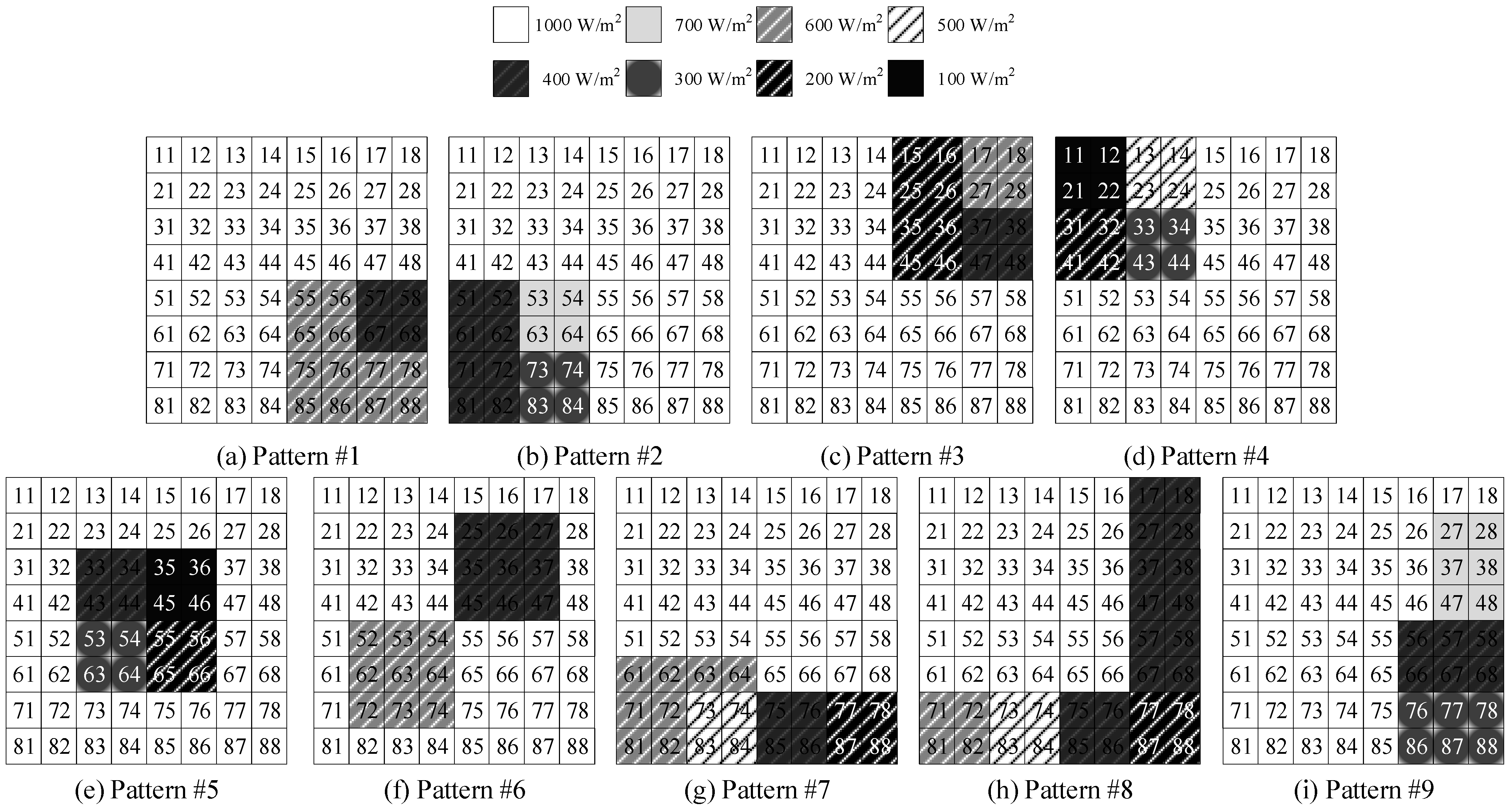
To assess the effectiveness of the MC-SDKP topology at mitigating the effects of shading and to compare its performance with that of four other topologies (TCT, Odd-Even, Optimal SDKP, and C-SDKP), an 8 × 8 PV array was tested under nine different patterns of partial shading and five different temperatures (increasing from 5 °C to 45 °C in increments of 10 °C). The estimation results showed that the PV array reconfigured with the MC-SDKP method generated the largest power output and the smallest difference in current on average. Thus, implementing the proposed method would lead to a decrease in the value of ΔIR and an increase in the reliability of the system. In addition, the results of the performance evaluation further confirmed that the MC-SDKP reconfiguration technique produced the largest average power output and power improvement (15.07%, and σ = 6.28%), and the smallest average power loss (1.34%, and σ = 0.99) of all five reconfiguration methods. Finally, the results of the box plot analysis of the power loss and improvement revealed that the MC-SDKP yielded the smallest distribution range and the fewest outliers among the five topologies, which confirmed its high degree of reliability under the test conditions.
Under Patterns #1, #3, #6, and #8, the MC-SDKP topology produced the highest power output among the five topologies which were examined. Moreover, under Patterns #3 through #5, the improvement in power output produced by the MC-SDKP was almost the same as that of the Optimal SDKP, which performed the best in response to these PSCs. In contrast to the performance of the TCT, the MC-SDKP boosted the output power by between 216 W and 850 W (i.e., 5.41–25.73%). It can be concluded that this study has succeeded in establishing the effectiveness of the MC-SDKP technique at mitigating the effects of both the center and corner shading of the PV array. Furthermore, using the MC-SDKP reconfiguration technique resulted in all the GMPPs being located or shifted to the LMPPs with the highest voltage in the case of all PSCs, which goes a long way towards simplifying the work of MPPT algorithms. The MC-SDKP topology was designed to be used for square sizes with an even number of both rows and columns, as it was in this study using an 8 × 8 PV array. Future research could be conducted to assess the performance of the MC-SDKP topology when it is used to reconfigure PV arrays of different sizes and implemented them in practice. The practical implementation of the proposed MC-SDKP topology to an 8 × 8 PV array is illustrated in
Figure A2 (
Appendix A).


