Abstract
To tackle the overheating problem of the heating surface in deep peak shaving, it is urgent to develop working substance (steam) temperature regulation and heating surface safety control technologies that combine combustion and hydrodynamic instability evaluation. This work relies on a 1000 MW boiler involved in deep peak shaving, and adopts CFD numerical simulation technology to obtain reasonable holographic heat load data of the boiler. The heat load data and the working substance side data are coupled to develop a real-time performance calculation model that combines combustion and hydrodynamic steam temperature. Real-time monitoring of the local position of the boiler water wall and the convection heating surface can be achieved through the three steps: heat load screening, heat exchange process calculation, and result display. The results show that through the corresponding expression of on-site industrial parameters and CFD simulation data, the effective analysis, extraction, modeling and optimization of the operation data can be realized for real-time online monitoring and intelligent early warning of the entire working condition. The model error is less than 2 °C and the model can realize early warnings at 5 min, so as to ensure the safety and stability of boiler operation and save the operating cost of the power plant to a certain extent.
1. Introduction
To achieve the global goal of “carbon neutralization”, renewable energies with large fluctuations and good intermittencies, such as wind energy and solar energy, are being increasingly connected to the grid for consumption, and the proportion of renewable energies has increased significantly. However, these renewable energies can cause unstable loading on the power grid. Coal power is the most economical and flexible resource with large-scale deep peak shaving capacity in China, and is the ballast for grid stability [1,2,3]. The intelligent and flexible transformation of coal power provides strong support for ensuring national energy security and achieving the dual carbon goals. The Action Plan for “Peaking Carbon Emissions before 2030 in China”, issued by the State Council in 2021, proposed to “Accelerate the energy-saving upgrading and flexible transformation of existing units”, and thus the development of coal-based flexible power generation technology is imminent. Coal-fired boiler rapid peak shaving technology is the key to improving the flexibility of coal-fired power units [4]. Because the boiler loading frequency under rapid-deep-peak regulation varies significantly, dynamic matching of combustion and heat transfer is high, and ensuring the safety of the water wall is difficult. Considering the huge size of the boiler and the complex internal high-temperature environment, it is neither economical nor realistic to arrange a large number of measurement points on the water wall to obtain the wall temperature distribution. In addition, the distributed control system (DCS) of the boiler can only reflect the macroscopic operating state of the unit, and cannot give the local temperature distribution of the pipe wall. Therefore, it is very necessary to establish a real-time hydrodynamic calculation model within the full load range of the water wall to provide data support for identifying and warning danger points, via clarifying the combustion flow heat transfer and energy flows under rapid variable load, and analyzing the mechanism of furnace combustion flow heat transfer under rapid variable load. Finally, problems such as overheating and pipe bursting should be solved to ensure the efficient and economical operation of the unit.
The overheating of a heating surface is mainly prevented through hydrodynamics, heating surface layout, combustion, etc., and the typical technologies include enhanced furnace water circulation technology and the water wall mixing arrangement method. However, ensuring the safety of a 15% ultra-low load heating surface is still a severe challenge [5,6]. In view of the above difficulties, as early as 1988, scholars [7] have published the life management and peak shaving operation methods of large-capacity thermal power units to guide the suppression of component stress fatigue damage. However, the frequent and rapid peak shaving of flexible units was only achieved by strengthening the furnace shutdown inspection to eliminate dangerous points. Aiming at the problem of alternating stress characteristics of turbine–generator sets under the interaction of flow, heat and solid, some have put forward the urgent need for innovative safety monitoring methods to cope with the new characteristics of rapid variable load, and some have proposed a monitoring method for key components of steam turbine generator sets with multiple information fusion, so as to explore effective control methods from the source to achieve unit safety and flexible collaboration [8,9].
At present, a large number of experts and scholars from all over word have carried out theoretical and simulation studies on the heat transfer and hydrodynamic characteristics of water walls [10,11]. The three-dimensional (3D) computational fluid dynamics (CFD) numerical simulation method is generally used for the study of the flue gas flow heat transfer process in the furnace [12,13]. However, CFD numerical research of boilers focuses on the flow combustion state of the flue gas side of the furnace. Although this can analyze the heat absorption deviation of the heating surface caused by the complex 3D flow and flue temperature distribution on the flue gas side, the detailed hydrodynamic parameters of the working fluid side are generally not included in the model, and the calculation of heat transfer on the heating surface is mostly based on the assumption of uniform distribution of working fluid temperature or pipe wall temperature in the tube [14]. Therefore, the influence of working fluid flow and temperature distribution in the pipe on the temperature of the pipe wall cannot be accurately reflected [15,16]. For the study of flow and heat transfer processes on the working fluid side, several one-dimensional hydrodynamic calculation methods are adopted [17,18]. Although the one-dimensional (1D) hydrodynamic calculation method can consider the flow and heat transfer processes on the working fluid side in detail, the heat flow distribution pattern of the furnace under different operating parameters is not included in the model [19,20]. Therefore, the influence of the heat absorption deviation of the heating surface on the wall temperature cannot be resolved [6,8]. In order to accurately predict the wall temperature distribution of the water wall, the three-dimensional heat flow distribution on the flue gas side and the flow and temperature distribution of the working fluid need to be included in the calculation model. However, the simultaneous simulation of the flue gas in the furnace and the flow heat transfer process of the working fluid in the pipe within the framework of the 3D CFD model leads to a huge number of meshes and calculations, due to the huge difference in the size of the furnace and the heating surface pipe. Many attempts have been made to couple 3D CFD models of the flue gas side of the furnace with the 1D hydrodynamic model of the working fluid in the tube, whose purpose is to realize the numerical simulation of the flow heat transfer process between the flue gas side and the working fluid side of the boiler [21,22]. Some foreign scholars have developed coupled heat transfer models and have studied the influence of pulverized coal radiation characteristics on furnace heat exchange. Some scholars have used coupling models to study the influence of flue gas recirculation on the distribution of heat flow in the water wall of secondary reheat boilers. However, these coupled models are mainly aimed at improving the prediction accuracy of boiler heat flow distribution, and still introduce different degrees of assumptions on the flue gas side or working fluid side. For example, the calculations in some studies are still based on the assumption of uniform working fluid temperature in the heated pipe, so the influence of working fluid temperature on the temperature of the pipe wall cannot be reflected in the calculation. However, some scholars have downgraded the heat flow distribution of the boiler heating surface to a one-dimensional distribution along the furnace height, which makes it impossible to analyze the influence of the heat absorption deviation of the flue gas side of the heating surface on the wall temperature. Although studies have shown that these simplifications have little impact on the prediction of the overall heat absorption of the heating surface [23], they ignore their important influence on the pipe wall temperature, making it impossible to accurately predict the pipe wall temperature.
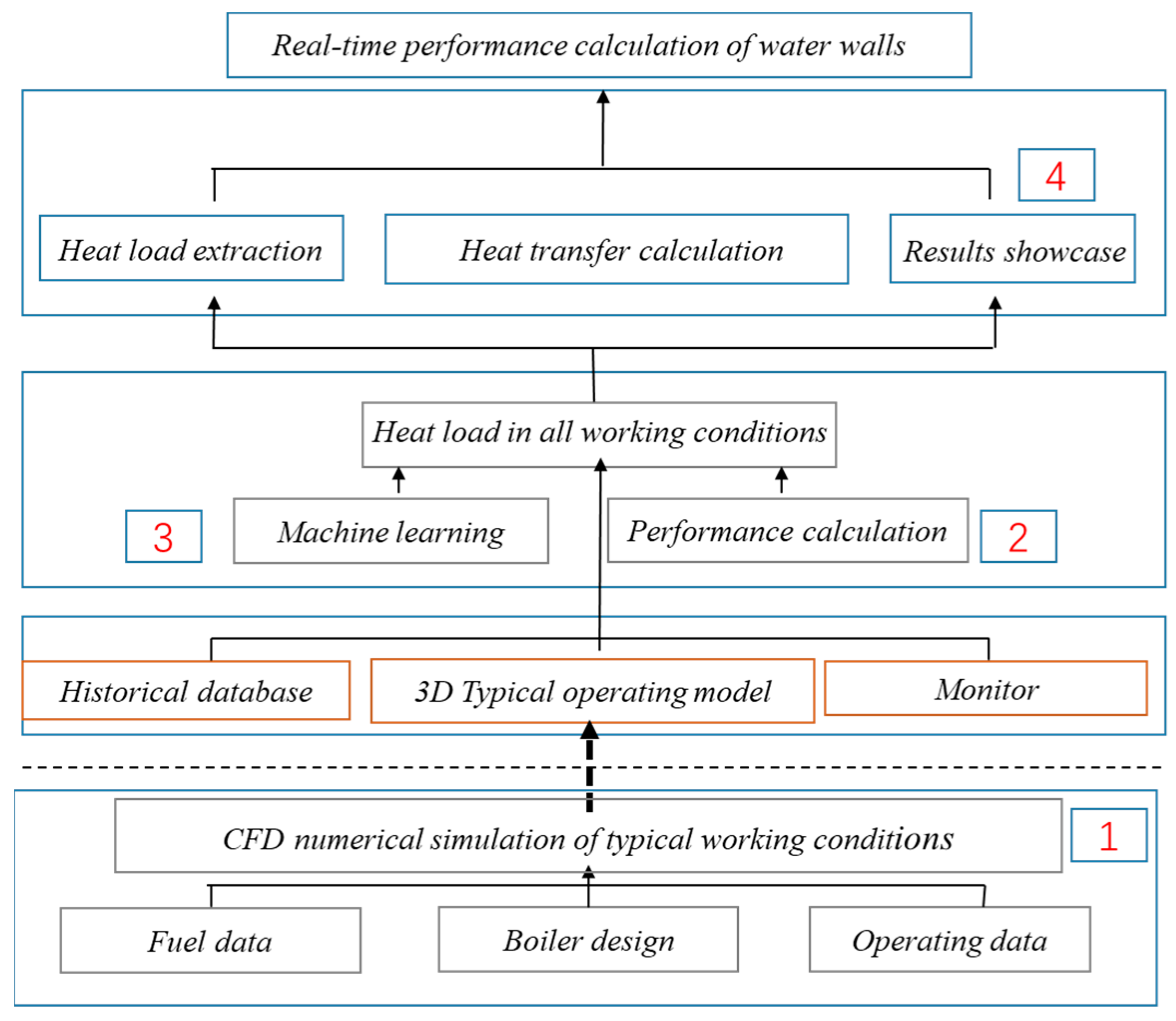
The burner in the furnace under the deep peak shaving condition is often not evenly input, the working fluid in the pot deviates from the designed working conditions, the combustion in the furnace is unsteady, the heat load is uneven and the water dynamic match in the pot is difficult, which often causes the heating surface to overheat [24,25]. Therefore, in this paper a real-time performance calculation method for coupling combustion and hydrodynamic steam temperature is proposed, and the technical route is shown in Figure 1. The reasonable holographic heat load data of the boiler are obtained through CFD numerical simulation technology, the heat load data are coupled with the working fluid side data, the on-site measurement point data are reasonably used, and the real-time performance calculation of the water wall is realized through the heat load screening and heat exchange process calculation. Furthermore, the development of this model is carried out on a 1000 MW boiler participating in deep peak shaving, and all heat load data are screened and distributed to each circuit in the heat load screening stage. In the calculation stage of the heat exchange process, according to the hydrodynamic calculation method, a calculation model of the working fluid heat exchange process is built to realize the calculation of temperature and pressure at any position of each circuit, according to the hydrodynamic calculation method. In the resulting display stage, the calculated temperature, pressure and other result data are displayed through the display platform to test the accuracy of the calculation results, and realize real-time monitoring of the overheating of the local position of the boiler water wall and convection heating surface.
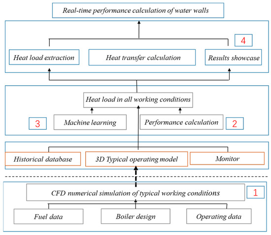
Figure 1.
Overall technical route.
2. Model Building
2.1. Project Introduction
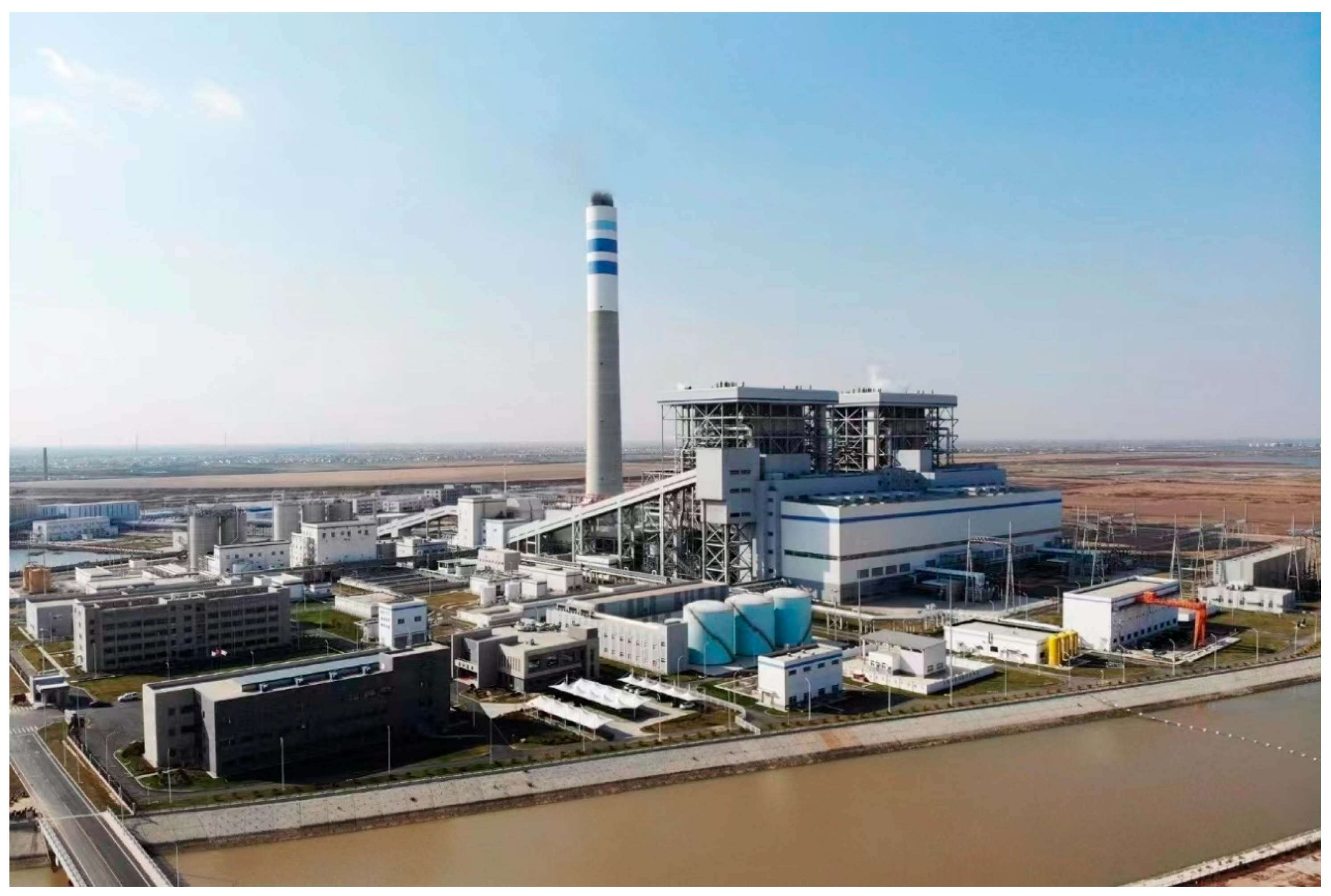
The parameters of the unit are 29.3 Mpa/605 °C/623 °C million high-efficiency ultra-supercritical DC (drect-current) boiler, and a diagram of the boiler is shown in Figure 2.
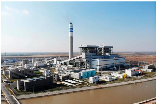
Figure 2.
Panorama of the 1000 MW unit.
This boiler adopts a Π-type arrangement, single furnace, primary intermediate reheating, low NOX main burner and high-level combustion exhaustion air graded combustion technology, with a reverse double-cut circular combustion mode. The furnace is a vertically rising membrane water wall of internal threaded pipe, without a circulating pump starting system. In addition to the coal/water ratio, the temperature control method also adopts a flue gas distribution baffle, burner swing, water spray and other methods. This machine group adopts a medium speed coal mill direct blowing mill milling system. Each furnace is equipped with 6 coal mills, 5 sets of operation, and 1 set of backup. The main operating data are shown in Table 1. The fineness of the pulverized coal is temporarily adjusted to R90 = 16%/15%, and the uniformity coefficient is 1.0~1.1; the coal using high ash bituminous coal is shown in Table 2.

Table 1.
Main operating parameters of boilers.
Table 2.
Coal quality data.
2.2. Data Preparation
The data foundation required for real-time wall performance calculations is collected and collated during the data preparation phase. The data required for real-time performance calculations of the water wall are divided into three categories: flue gas side data, working fluid side data, and boiler structure data.
The flue gas side data refer to the heat load distribution data required for the real-time performance calculation of the water wall, which means the heat exchange value at each position of the water wall, which is calculated based on CFD numerical simulations. The working fluid side data refers to the measurement data of the working fluid at each key point of the water wall part, such as the temperature at the water wall inlet header, the pressure at the water wall inlet header, the flow rate at the water wall inlet container, etc. These data come from the measurement point data during boiler operation and are collected from the DCS system of the power plant. Boiler structure data refer to the design information of the water wall, including the steam flow chart, spiral pipe ring layout size, header position, pipe diameter, and other information, which come from the boiler design unit. Data preparation summarizes the above three types of data, cleanses and processes abnormal data, and converts these data into the format required for calculation. The calculation principle is shown in Figure 3.
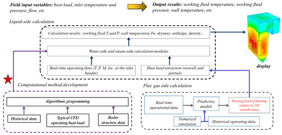
Figure 3.
Calculation principle.
2.3. Circuit Division
Water wall circuit division: the normal water wall hydrodynamic calculations to divide the circuit are generally 20–30 pipes a circuit, pipe spacing of about 38 mm, a circuit width of 700–1000 mm, boiler CFD calculation due to the large size of the furnace, and the general grid scale is 200–300 mm. According to this circuit, there are only 2–3 grids, so the normal hydrodynamic calculation to divide the water wall circuit is not applicable. Therefore, 2–3 circuits are selected in the water wall calculation to form a large circuit, and the working fluid heat absorption on the large circuit is calculated. The main workload of the circuit division is to construct the mathematical expression of each loop; the function of the expression is used as the basis for filtering the data in the CFD numerical simulation results, and the heat exchange value (Heat-flux) required by each circuit of the load can be filtered out according to the coordinate information (x, y, z) through the Python language. The method of constructing the mathematical expression of each circuit is shown in Figure 4.
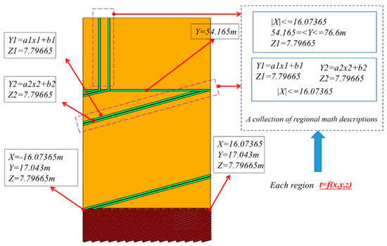
Figure 4.
Construction method of loop mathematical expression.
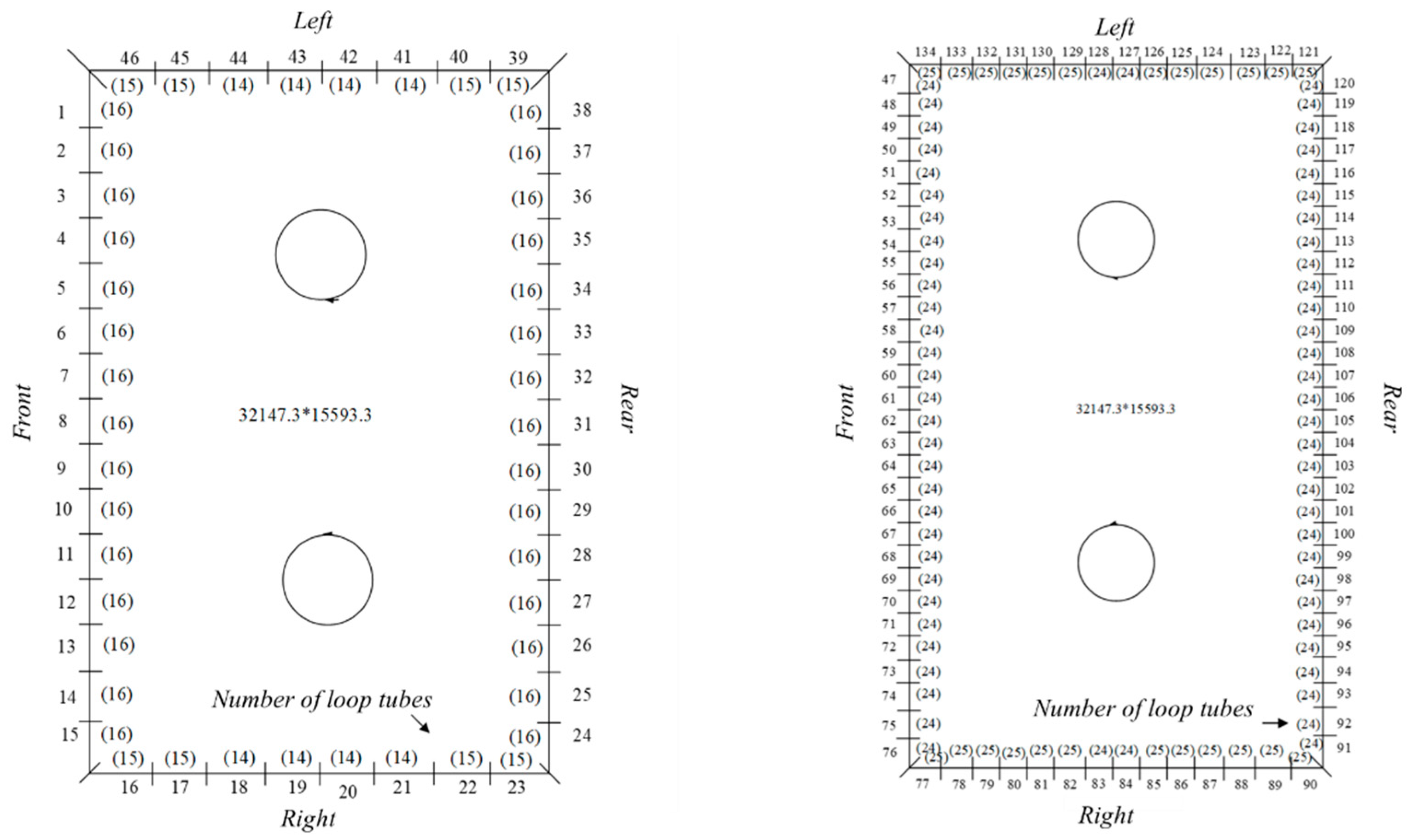
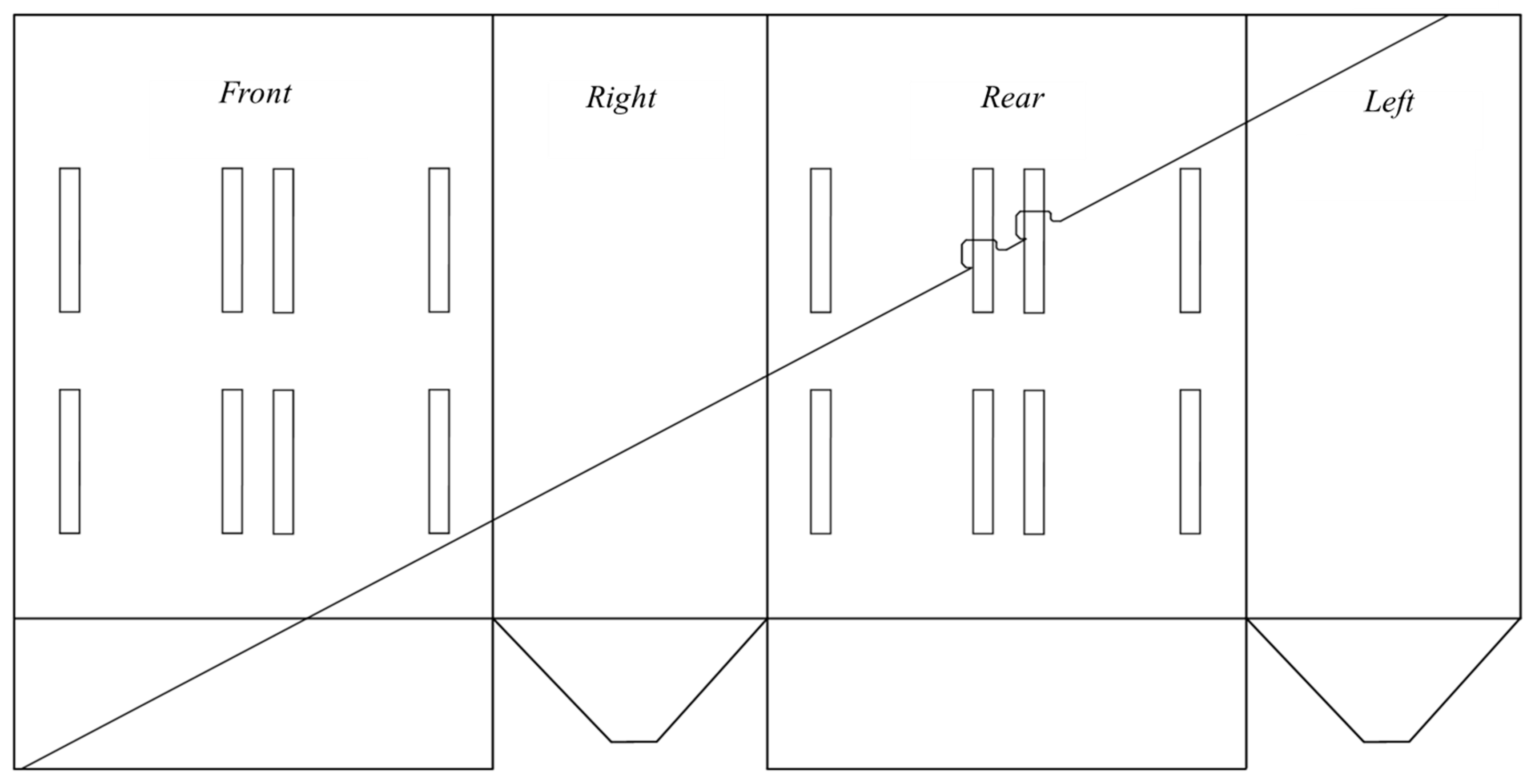
Figure 5 (left) shows a schematic diagram of the calculation loop division of the lower furnace spiral coil. The spiral pipe ring of the front wall and back wall of the lower furnace is divided into 15 circuits, and the side wall is divided into 8 circuits, for a total of 46 circuits. Combined with the heat load distribution curve of the furnace, the number of tubes in each circuit is distributed. The peripheral number in the figure is the circuit number, and the parenthetical number in the inner circle corresponding to the position is the number of tubes in the loop. Among them, 1~15 circuits are arranged on the front wall, 16~23 circuits are arranged on the right wall, 24~38 circuits are arranged on the back wall, and 39~47 circuits are arranged on the left wall. The tube specifications of the lower furnace spiral ring are lower Φ38 × 7.3 mm and upper Φ38 × 8 mm, with a pitch of 53 mm and an inclination angle of 23.391, for a total of 712 pieces. The spiral pipe ring spirals from the inlet of the cold ash hopper to the middle header of the water wall. Figure 5 (right) is a schematic diagram of the calculation loop division of the vertical pipe ring of the upper furnace. The vertical pipe ring of the upper furnace is led out by the middle header of the water wall, and there are 2136 pipes divided into a total of 88 circuits. The tube size is Φ28.6 × 5.8 mm and the pitch is 44.5 mm.
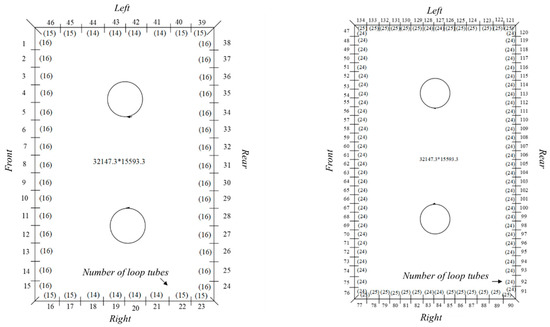
Figure 5.
Schematic diagram of the vertical pipe ring circuit division of the furnace under.
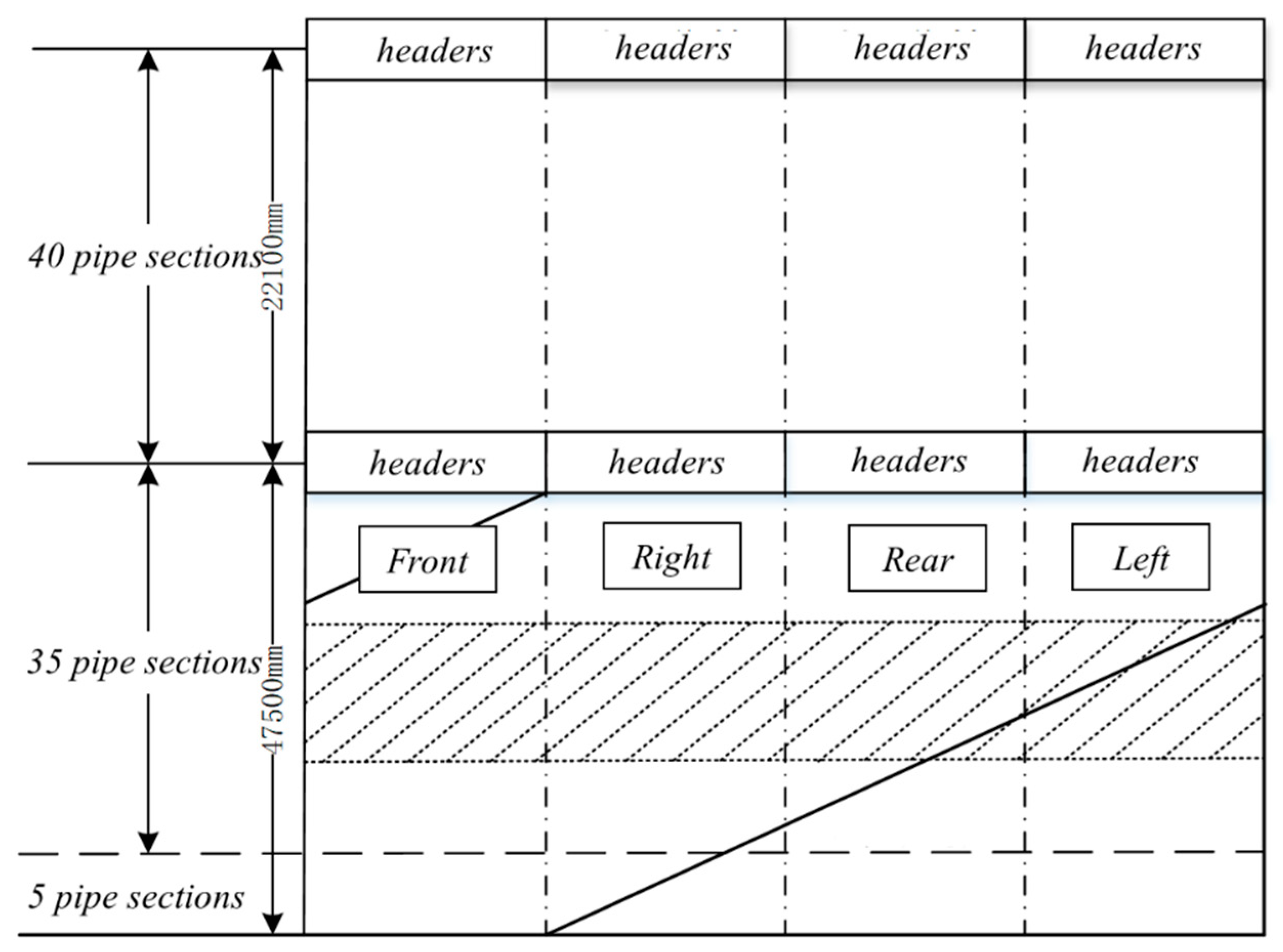
The lower furnace circuit is divided into 40 pipe sections. The water-walled pipes below the inflection point of the cold ash hopper were divided into 5 pipe segments. From the inflection point of the cold ash hopper to the water wall spiral coil at the header in the middle of the water wall, each circuit is divided into 35 pipe segments. Each circuit of the furnace is divided into 12 pipe sections. The schematic diagram of the division of the pipe section is shown in Figure 6.

Figure 6.
Schematic diagram of the division of pipe segments.
According to the division of the calculation loop of the lower furnace spiral pipe ring water wall in Figure 5, the lower furnace water wall is specially drawn along the coiled direction of the furnace so that the direction of the spiral pipe ring can be clearly seen, as shown in Figure 7. The lower furnace chamber shown in the figure is the transition section from the inflection point of the cold ash hopper to the spiral pipe ring and the vertical pipe segment. The figure is the lower furnace spiral pipe ring starting from the front wall, right wall, back wall, and left wall along the direction of the furnace, and the division of each circuit in the figure is consistent with the circuit division number in Figure 5.

Figure 7.
The expansion diagram of the water-cooled wall.
Based on the calculation of the above fluent software, the combustion process of coal powder in the boiler was obtained. When developing real-time performance calculation algorithms for water side and steam side models, heat load distribution data were used. In order to facilitate the use of heat load data, fluent software has its own functions to convert distribution trends into binary ASCII format files. The converted data have four columns: x, y, z, and Heat flux. The first three items refer to the coordinates of the point, in m. The last item refers to the value of heat exchange, expressed in kW/m2. The specific data format is shown in Table 3.
Table 3.
Data format table of numerical simulation calculation results.
The construction of the water side model mainly involves the division of hydrodynamic circuits, and its main workload lies in the construction of mathematical expressions for each circuit. The function of this expression is to serve as a screening basis for data in CFD numerical simulation results. Through the Python language, the required heat exchange values (Heat flux) for each circuit of the load can be filtered out based on coordinate information (x, y, z), and the mathematical expressions for each circuit can be constructed. The mathematical expressions for each circuit are expressed in the form of y = ax + b, so the focus of circuit division is to solve for a and b at the upper and lower boundaries of each circuit, where a is the slope of the corresponding circuit segment. The solution process is implemented using Python, and the calculation results are stored in the dictionary DICT in Python. The expansion diagram of the water-cooled wall is shown in Figure 7: with the upper corner as the origin, the right horizontal coordinate x, and the downward vertical coordinate y, establish a segmented equation of y = ax + b. The points on this line represent the physical location of a certain section of a circuit. According to the data in DICT, during the processing of CFD data, the heat load values within each circuit range were filtered out, which solved the heat in each circuit. Then we placed the calculated heat load data in this coordinate system, so that the heat load point corresponds to the circuit pipe segment.
2.4. Calculation Model
2.4.1. Calculation Method for Flue Gas Side Heat Transfer
As a radiation heating surface, the furnace can be calculated using a flame radiation heat transfer equation proportional to the fourth power of temperature, and then based on time:
In the equation, the radiation constant of the absolute blackbody , furnace blackness , represents the flame temperature, represents the wall temperature, H represents the heat exchange area, and is the calculated fuel quantity.
The convective heating surface still divides the heat transfer on the heating surface into two parts for calculation: flue gas side heat transfer and working fluid side heat transfer. Consider the following equation:
In the equation, is the thermal conductivity of the metal, is the outer diameter of the metal pipe, Re and Pr are the flue gas Reynolds number and Ludwig Prandtl number, CS is the correction factor for the geometric arrangement of the tube bundle, CZ is the correction coefficient for the number of pipe rows on the flue gas stroke, TY is the flue gas temperature, a is the flue gas blackness, and the above parameters are calculated according to the boiler thermal calculation standard.
2.4.2. Fluid Flow and Heat Transfer Model
The working fluid flowing in the pipe can be simplified as the momentum, energy and continuity equation obeyed by the one-dimensional model:
In the formula, is the pipeline direction unit vector; is the flow velocity of the fluid inside the pipe; is the pipeline flow area; , , , are the thermal conductivity, specific heat at constant pressure, fluid density and Ludwig Prandtl number of the fluid, respectively; and fluid pressure are interpolated in the parameter table exported by NIST software; is the inner diameter of the pipe; is the heat load per unit length; is the Darcy coefficient, , represents gravity.
The heat absorption of the furnace heating surface can be simplified based on the average heat load of the furnace given by thermodynamic calculations. For the convective heating surface of the horizontal flue, the temperature field is given based on thermodynamic calculations, and the heat transfer process is considered according to the following equation:
In the equation, is the thermal conductivity of the metal on the pipe wall.
3. Results and Discussion
3.1. Boiler Physical Model and Operating Parameters
The boiler geometry is shown in Figure 8. The main burner adopts the traditional large bellows structure, and the large bellows are divided into several air chambers by the partition, including one OFA air chamber, one upper end air chamber, six pulverized coal air chambers, eighteen intermediate air chambers, twenty-one middle air chambers, one oil air chamber, two intermediate oil air chambers, and one lower end air chamber. According to the height of each wind chamber, the arrangement of nozzles is shown in the figure on the right. The arrangement of the OFA combustion air chamber at the upper end of the burner controls the NOX emissions, and the setting of two groups of SOFA winds above the main burner further reduces the NOX emissions. The burner pull-open arrangement and reasonable air distribution form can effectively control NOX emissions [26]. We calculated the boundary conditions to ensure that the burner inlet air speed is the design value (see Table 4).
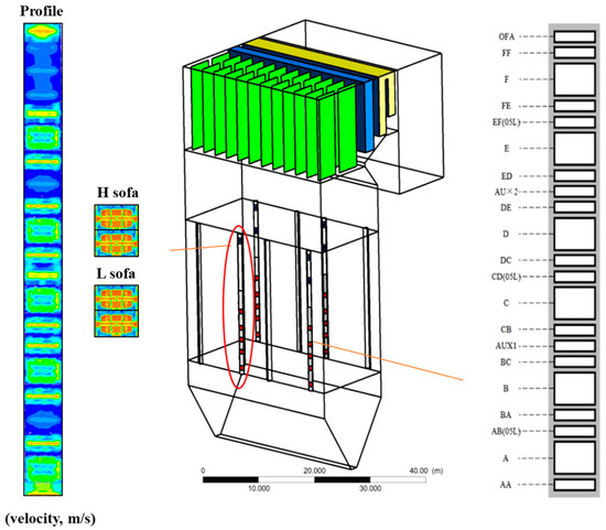
Figure 8.
Schematic diagram of boiler burner and heating surface arrangement.
Table 4.
Calculated boundary conditions.
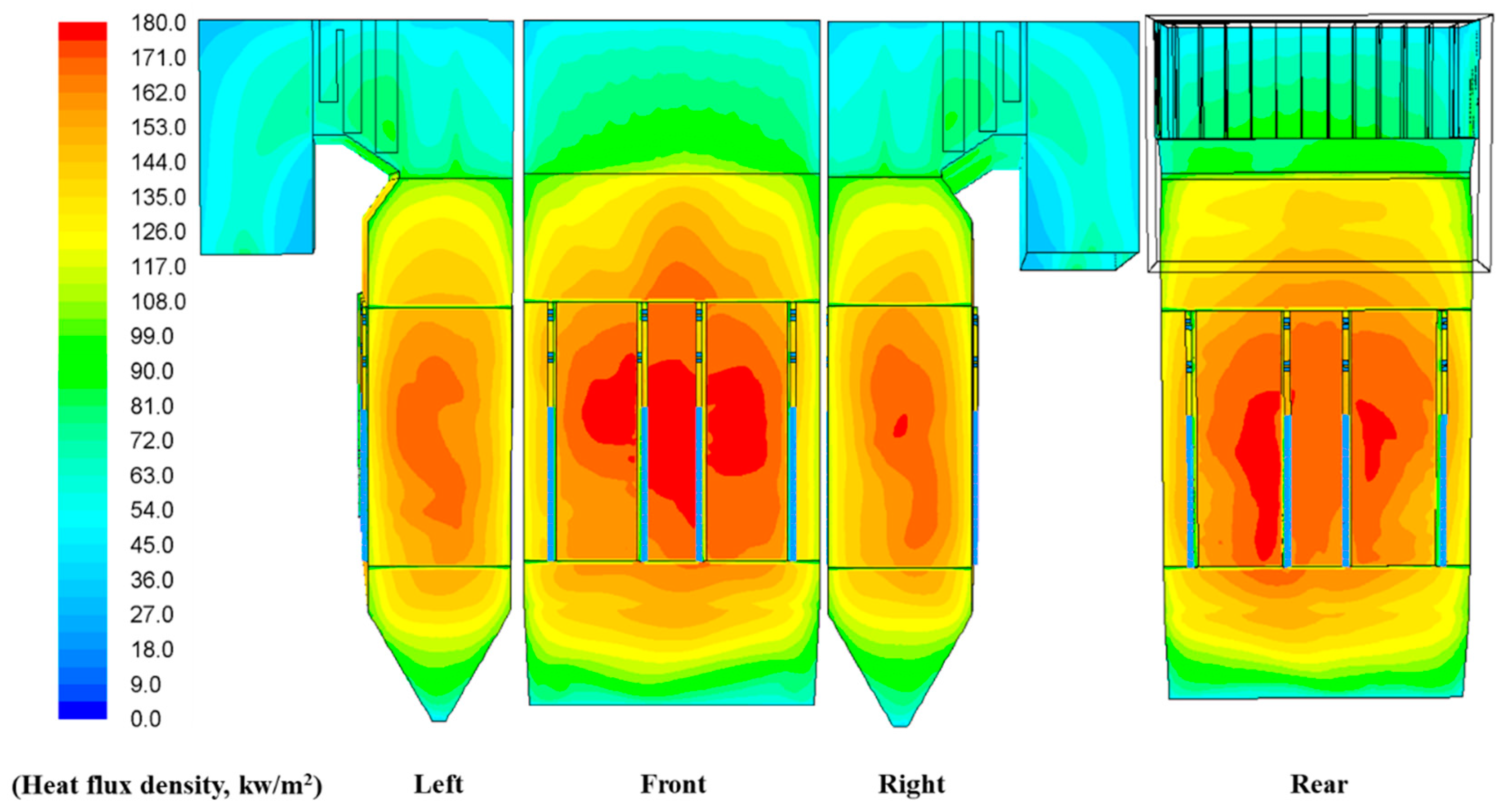
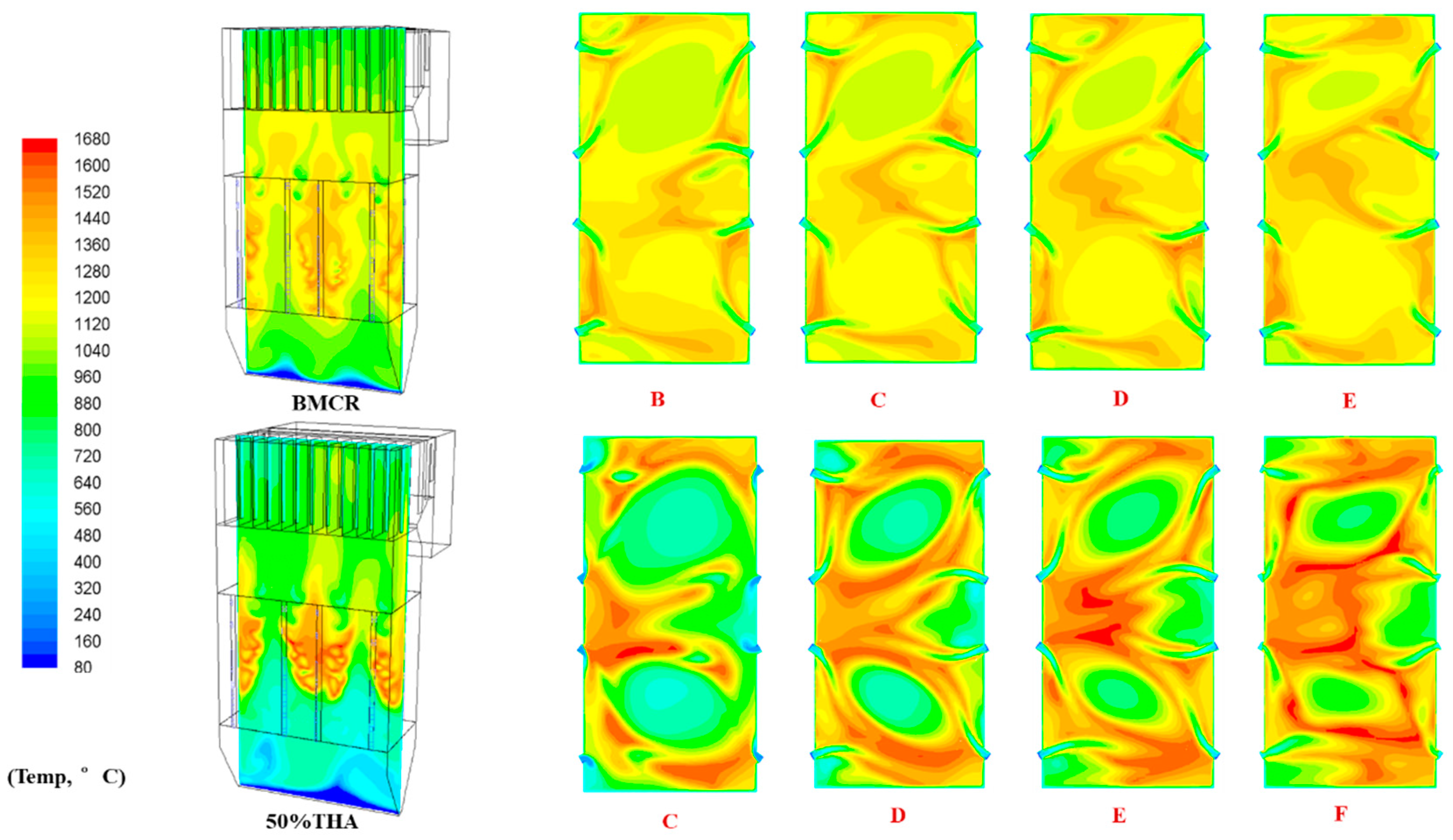
The three-dimensional CFD numerical model of the flue gas side can be found in the literature [17,19]. After the calculation of fluent software, the combustion process of pulverized coal in the boiler is obtained, the heat load distribution data are used when developing the real-time performance calculation algorithm of the water wall, and the three-dimensional display of the calculation result is shown in Figure 9. The highest heat flux density of the furnace wall occurs in the area near the burner on the top floor of the front wall and the separation burnout wind, corresponding to the area with the highest flame temperature of the furnace.

Figure 9.
Boiler heat load distribution diagram.
3.2. Heat Load Screening
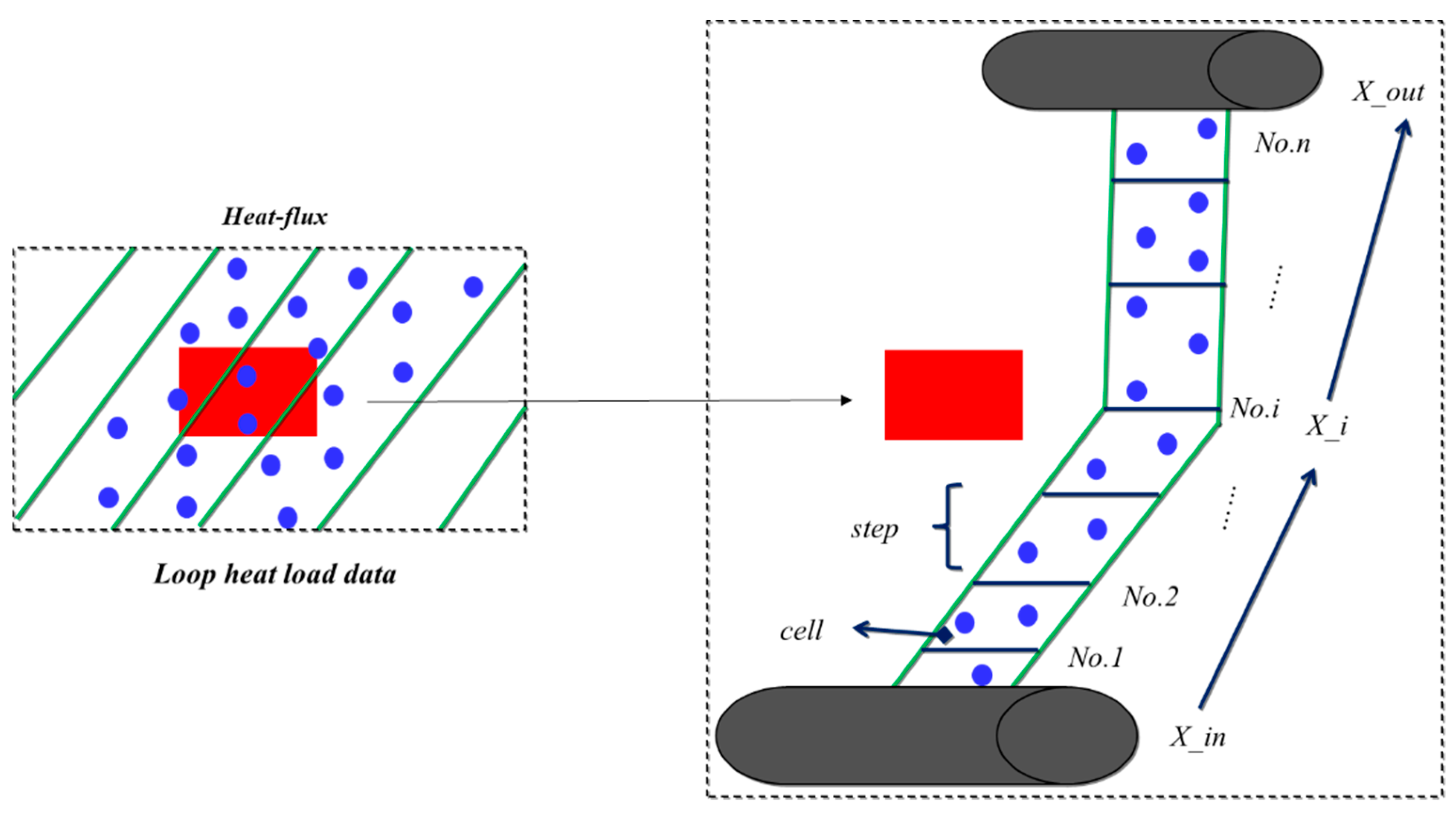
In order to facilitate the use of heat load data, the distribution trend is converted into a binary ASCII format file by using the fluent software’s function, and the converted data have four columns: x, y, z, and heat-flux. The first three refer to the coordinates of the point in m. The last item refers to the value of heat exchange, which is measured in kW/m2. According to the data in the dictionary DICT of Table 3 in the data processing in CFD, the heat load value in each loop range is filtered, and the heat in each loop is solved. The screening process is shown in Figure 10.
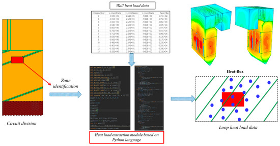
Figure 10.
Heat load data screening process.
The wall heat load data are imported into the program, and the program will extract the heat load according to the divided circuit, and calculate the working fluid temperature and wall temperature. When the operator wants to view the heat load and wall temperature of a certain area, the program will identify the area, determine the constraint range, and automatically extract the heat load and wall temperature of the corresponding area for display.
3.3. Heat Transfer Process Calculation
3.3.1. Flow Resistance Calculation
The working fluid in the boiler tube has both single-phase fluid and vapor–liquid two-phase fluid, which will produce a certain pressure drop due to the need to overcome various resistances when flowing in the tube. According to the momentum conservation equation, the basic equation for the calculation of pressure drop in boiler hydrodynamic calculations is:
where ∆p is the total pressure drop, which is defined as the difference between the pressure at the beginning and end of the pipeline. ∆pmc and ∆pjb represent frictional resistance and local resistance, respectively, and the sum of these two is usually called flow resistance ∆pu; ∆pzw and ∆pjs are called heavy pressure drop and accelerated pressure drop, respectively.
∆p = ∆pmc + ∆pjb + ∆pzw + ∆pjs
3.3.2. Calculation of Heat Transfer in the Tube
The temperature rise calculation of the working fluid is calculated using the following formula:
where Q is the total heat, that is, the result of heat load screening, Q = Heat-flux × A, A is the loop area, obtained in the boiler structure data. c is the constant pressure-specific heat of working fluid, which is queried using the iapws module, which is a library file for Python. m is the working fluid flow, obtained in the operating data section.
Q = c × m × ∆t
3.3.3. The Program Performs Calculations
The execution of the hydrodynamic calculation method is shown in Figure 11. The previous calculation of steps is written in the Python language, forming a script file with the suffix.py, which is run in the Python 3.5 environment. The execution steps are: 1. Read the data measurement point data at the inlet header of the water wall; 2. Read the heat load screening result data; 3. Set the calculation step in the height direction; 4. Calculate the pressure drop; 5. Calculate the temperature; 6. Query parameters; 7. Cyclic calculation improves calculation accuracy; 8. Numerical test of measurement points.

Figure 11.
Hydrodynamic calculation execution.
The temperature and pressure values at each position of the vertical section and the spiral section of water wall can be obtained, and the real-time performance calculation of the water wall is completed [27]. In order to facilitate the observation of the overall distribution trend of temperature, the calculation results are displayed in a three-dimensional visualization platform, and the display effect is shown as shown in 12. The display interface in Figure 12 is divided into two parts: the left part shows the overall temperature distribution trend of the spiral segment and the vertical segment, and the right part shows the local display of a part of the spiral segment and vertical segment that can be selected by the user.
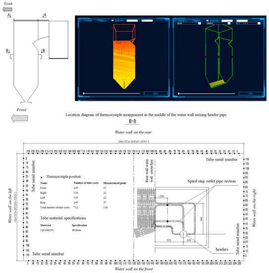
Figure 12.
Real-time performance calculation of water wall.
To verify the correctness of the selected calculation model, the experimental measurements of the boiler under BMCR (boiler maximum continuous rating) load were compared with the numerical simulation results, as shown in the table below. From Table 5, it can be seen that the flue gas temperature at the furnace outlet, and working fluid temperature at the outlet are basically the same: the simulated flue gas temperature is slightly higher than the operating value, with a relative error of less than 5%; The relative error of the working medium temperature shall not exceed 2%. Therefore, the numerical simulation model selected in this article has high credibility.
Table 5.
Comparison between simulation and practice.
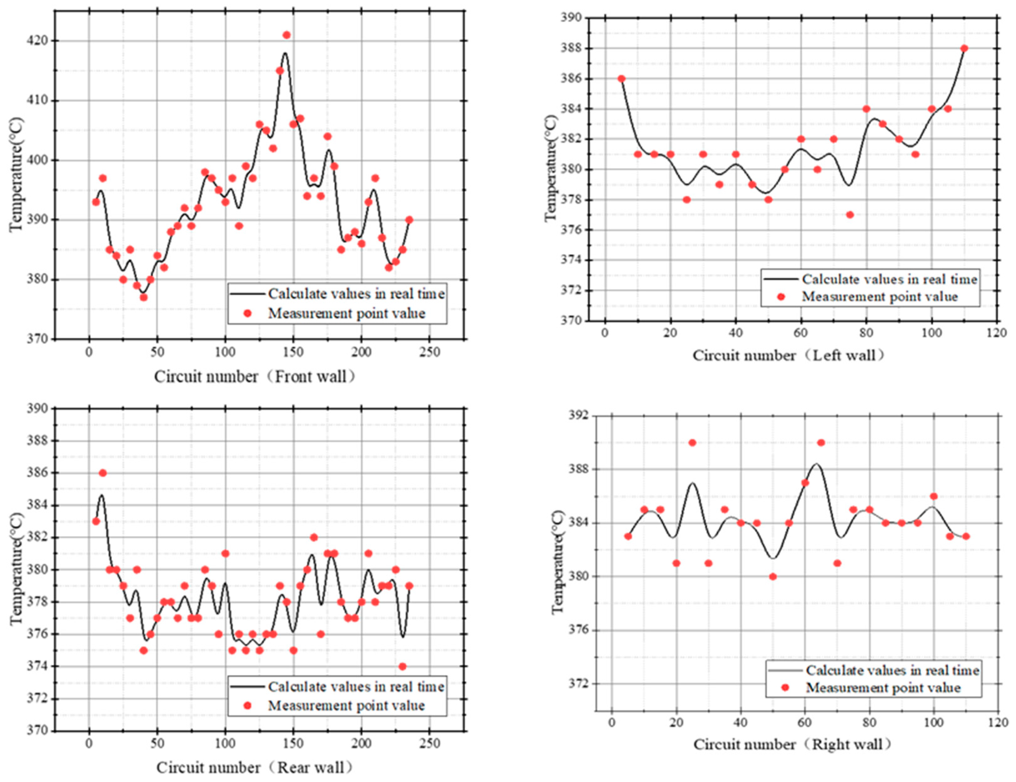
The layout diagram of the on-site water-cooled wall measurement point is shown in Figure 13, intercepting the load operation conditions of the 550 MW unit on site, and the calculation results of the outlet wall temperature of the water-cooled wall according to the feedback of the on-site measurement point data are in good agreement with the measurement data. The error is within 2 °C, which verifies the accuracy of the coupling model. The calculation of full coverage of the wall temperature of the water-cooled wall pipe except the measurement point is realized.
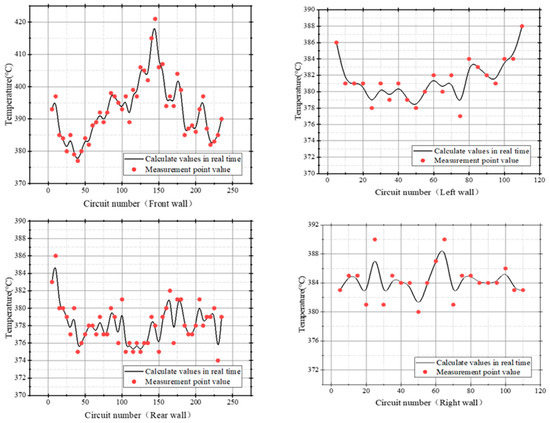
Figure 13.
On-site water-cooled wall measurement point layout.
Figure 14 shows the distribution law of each burner section: from the temperature distribution law, it can be seen that there is a hot and cold angle law for the octagonal reverse double-cut circular furnace, which is consistent with the actual operation. The simulation shows that the temperature located in the center of the furnace is lower than the ambient temperature. The reason for this is that the distribution of pulverized coal particles in the center of the furnace is small, and the heat released is limited, so the temperature of the center of the section is low and the temperature is high. In the main combustion area of the furnace, a large amount of primary wind is replenished, which accelerates the ignition and combustion of pulverized coal particles and promotes the combustion and heat release of pulverized coal. Therefore, the formation of a high-temperature area and the high-speed rotation of the flue gas helps to ignite the coal powder injected into it and improve the mixing effect of pulverized coal, so the fire in this area is more easily caused and the flow field is stable. However, the front wall adhesion is more obvious.
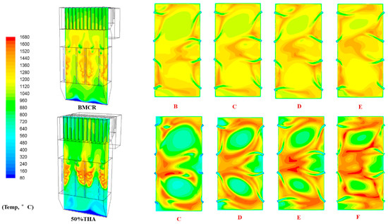
Figure 14.
Cross-sectional distribution of burner.
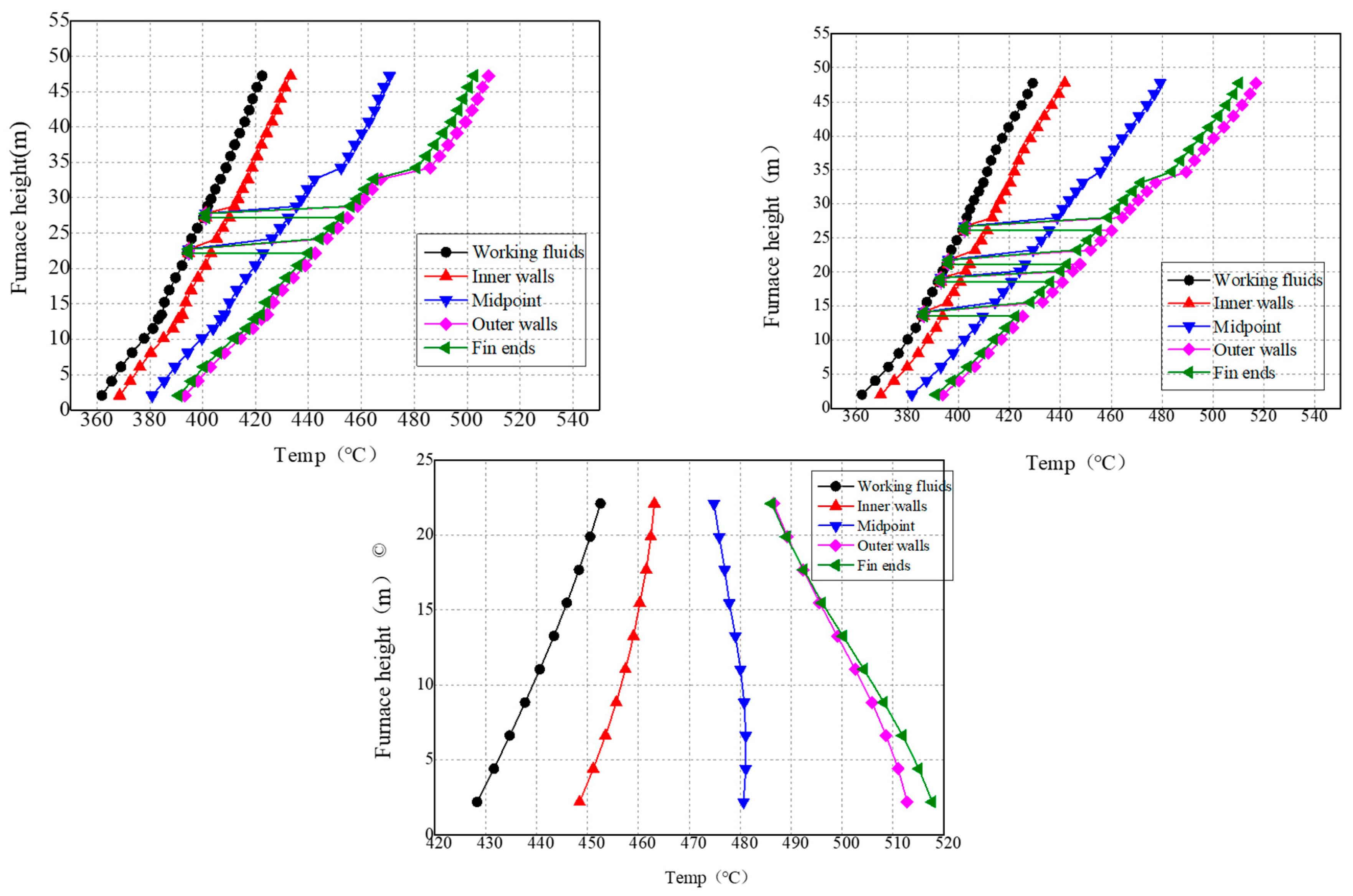
According to the calculation results, the pipe with a high water wall temperature under medium and low load is roughly fixed and is little affected by different grinding combinations, the upper swing of the main burner and other conditions. The temperature margin of the front wall is relatively small, the wall temperature margin of the back wall is temperate and the wall temperature margin of the two sides is large. The pipe with high wall temperature of different grinding combinations is not the same. For the analysis of wall temperature distribution under BMCR load, the 15th circuit of the longest pipe and the sixth circuit of the shortest tube of the front wall were selected as the wall temperature analysis objects of the spiral pipe coil. The temperature analysis object of the vertical water-cooled wall pipe of the upper furnace was selected as the 60th circuit of the heated strongest pipe of the front wall for analysis. Figure 15 shows the variation curves of wall temperature in the direction of furnace height in the lower furnace circuit, circuit 15 and upper furnace circuit 60 under BMCR loading, respectively.
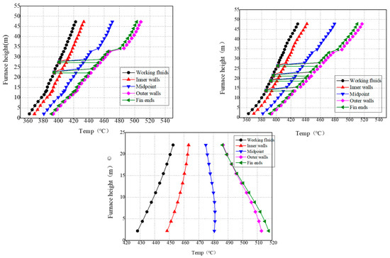
Figure 15.
Wall temperature change curve under BMCR condition.
Taking the 15th circuit as an example, it can be seen that under BMCR load, the working fluid was in the single-phase zone, so the working fluid temperature increases with the increase of the furnace height, and the wall temperature also increases. The temperature point that suddenly decreases in the figure is the unheated pipe section that bypasses the burner, and the working fluid temperature, inner wall temperature, intermediate point temperature, outer wall temperature, and fin temperature coincide into one point. At the furnace height of 47.24 m, the temperature of the outer wall of the metal reaches a maximum value, which is about 516 °C. At this time, the midpoint temperature also reaches a maximum of 479.3 °C.
For the upper furnace, taking the 60th circuit as an example, it can be seen that the working fluid temperature increases with the increase of the furnace height, but the wall temperature is gradually reduced by the influence of the heat load with the decrease of the height. The outer wall temperature of the maximum temperature of the upper furnace reaches 512.8 °C, the maximum temperature of the middle point is 481.1 °C, and the maximum temperature of the fin end is 517.7 °C.
For the calculation of wall temperature, for the lower furnace, the wall temperature of the lower furnace above the burner is high, the maximum intermediate point wall temperature of each circuit is 479.3 °C, the maximum outer wall temperature is 516 °C, the maximum fin temperature is 510 °C, and the selection of 15CrMoG can meet the safety requirements. For the furnace, the maximum intermediate point wall temperature of each circuit is 481.1 °C, the maximum outer wall temperature is 512.8 °C, the maximum fin temperature is 517.7 °C, and the selection of 12Cr1MoVG can meet the safety requirements.
In general, when the BMCR is loaded, it is safe and reliable to use 15CrMoG and 12Cr1MoVG for the boiler furnace.
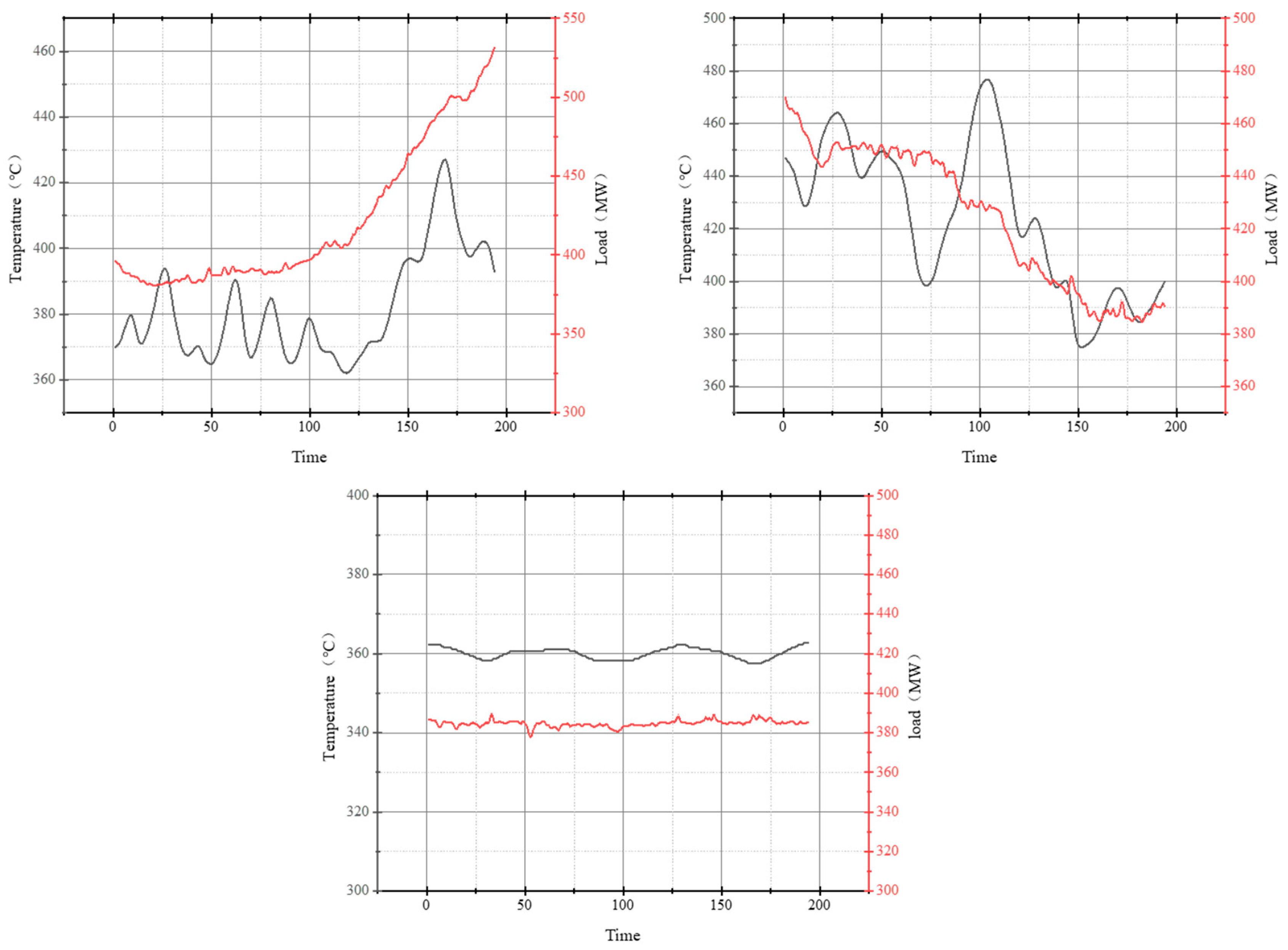
At present, the minimum depth adjustment capacity of the unit can be as low as 380 MW, and the real-time calculation of the 1000 MW boiler using this model is shown in Figure 16. According to the real-time calculation model, the unit is safe and reliable.
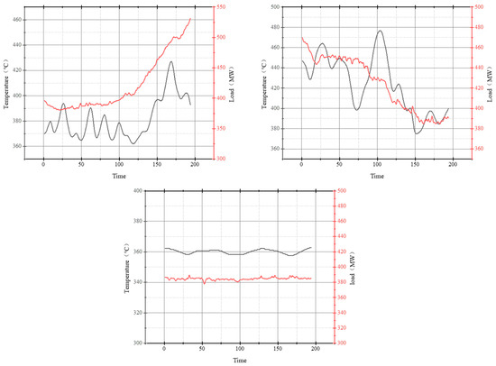
Figure 16.
Wall temperature change curve under variable working conditions.
4. Conclusions
In order to solve the problem of overheating of the heating surface during deep peak shaving of boilers, this paper proposes a real-time calculation of steam temperature that couples combustion and hydrodynamic instability evaluations. This model uses a three-dimensional CFD model to obtain the three-dimensional distribution of flow and heat transfer on the boiler flue gas side, and uses Python software to construct a one-dimensional flow and heat transfer model on the working fluid side of the boiler. The two models can accurately predict the temperature distribution of the working medium in the heating surface tube and the tube wall through the data interaction between the heat flow density of the heating surface and the temperature of the working medium in the tube, and accurately reflects the influence of the heat transfer deviation at the flue gas side caused by the complex flow field in the furnace and the flow deviation of the working medium in the tube on the temperature distribution of the tube wall of the heating surface, to accurately predict the overheating area of the tube wall of the heating surface.
- The coupled model was used to numerically simulate the heat transfer and wall temperature distribution of a 1000 MW boiler’s water-cooled wall. The calculated and measured results of the boiler’s smoke temperature distribution and wall temperature distribution under different loads were in good agreement. The true wall temperature of the full screen tube was within 2 °C, and the accuracy of the model was verified.
- We utilized machine learning algorithms based on embedded mechanism models to achieve real-time online visualization prediction of flow temperature, pressure, and wall temperature in pipes at different local overheating positions of water-cooled walls. At the same time, based on the full working condition databases of flue gas and working fluid sides in the furnace and select characteristic variables, we constructed a unit control system based on the 3D distribution of heat load in the furnace to achieve safe and stable operation of the unit at 15–110% rated load.
Author Contributions
Conceptualization, G.Z.; Methodology, X.G.; Software, X.G.; Validation, G.Z.; Investigation, Z.Z. (Zhengshun Zhang); Resources, Z.Z. (Zhecheng Zhang); Writing—original draft, X.G.; Writing—review & editing, D.F.; Supervision, Y.W. All authors have read and agreed to the published version of the manuscript.
Funding
This work was supported by the National Key R&D Program of China (2022YFB4100600) and Fundamental Research Funds for the Central Universities (FRFCU5710051521).
Conflicts of Interest
The authors declare no conflict of interest.
References
- Zhou, S.; Wang, Y.; Zhou, Y.; Clarke, L.E.; Edmonds, J.A. Roles of wind and solar energy in China’s power sector: Implications of intermittency constraints. Appl. Energy 2018, 213, 22–30. [Google Scholar] [CrossRef]
- Liu, L.; Wang, Z.; Wang, Y.; Wang, J.; Chang, R.; He, G.; Tang, W.; Gao, Z.; Li, J.; Liu, C. Optimizing wind/solar combinations at finer scales to mitigate renewable energy variability in China. Renew. Sustain. Energy Rev. 2020, 132, 110151. [Google Scholar] [CrossRef]
- Henderson, C. Increasing the flexibility of coal-fired power plants. IEA Clean Coal Cent. 2014, 15, 15. [Google Scholar]
- Huang, C.; Zhang, P.; Wang, W.; Huang, Z.; Lv, J.; Liu, J.; Ni, W. The upgradation of coal-fired power generation industry supports China’s energy conservation, emission reduction and carbon neutrality. Therm. Power Gener. 2021, 50, 1–6. [Google Scholar]
- Guo, X.; Zhao, G.; Sun, Z.; Song, B.; Guo, J.; Zhao, Z.; Li, H. Effect of Recirculated Flue Gas on Steam Parameters of 660 MW Double Reheat Boiler. Proc. CSEE 2018, 38, 1101–1110. [Google Scholar]
- Xiong, T.; Yan, X.; Huang, S.; Yu, J.; Huang, Y. Modeling and analysis of supercritical flow instability in parallel channels. Int. J. Heat Mass Transf. 2013, 57, 549–557. [Google Scholar] [CrossRef]
- Shen, Z.; Yang, D.; Wang, S.; Wang, W.; Li, Y. Experimental and numerical analysis of heat transfer to water at supercritical pressures. Int. J. Heat Mass Transf. 2017, 108, 1676–1688. [Google Scholar] [CrossRef]
- Shen, Z.; Yang, D.; Xie, H.; Nie, X.; Liu, W.; Wang, S. Flow and heat transfer characteristics of high-pressure water flowing in a vertical upward smooth tube at low mass flux conditions. Appl. Therm. Eng. 2016, 102, 391–401. [Google Scholar] [CrossRef]
- Liu, P.; Hou, D.; Lin, M.; Kuang, B.; Yang, Y. Stability analysis of parallel-channel systems under supercritical pressure with heat exchanging. Ann. Nucl. Energy 2014, 69, 267–277. [Google Scholar] [CrossRef]
- Wu, X.; Fan, W.; Liu, Y.; Bian, B. Numerical simulation research on the unique thermal deviation in a 1000 MW tower type boiler. Energy 2019, 173, 1006–1020. [Google Scholar] [CrossRef]
- Tan, P.; Fang, Q.; Zhao, S.; Yin, C.; Zhang, C.; Zhao, H.; Chen, G. Causes and mitigation of gas temperature deviation in tangentially fired tower-type boilers. Appl. Therm. Eng. 2018, 139, 135–143. [Google Scholar] [CrossRef]
- Yang, X.; Ingham, D.; Ma, L.; Zhou, H.; Pourkashanian, M. Understanding the ash deposition formation in Zhundong lignite combustion through dynamic CFD modelling analysis. Fuel 2017, 194, 533–543. [Google Scholar] [CrossRef]
- Boyd, R.; Kent, J. Three-dimensional furnace computer modelling. Symp. (Int.) Combust. 1988, 21, 265–274. [Google Scholar] [CrossRef]
- Gao, N.; Jia, X.; Gao, G.; Ma, Z.; Quan, C.; Naqvi, S.R. Modeling and simulation of coupled pyrolysis and gasification of oily sludge in a rotary kiln. Fuel 2020, 279, 118152. [Google Scholar] [CrossRef]
- Starkloff, R.; Alobaid, F.; Karner, K.; Epple, B.; Schmitz, M.; Boehm, F. Development and validation of a dynamic simulation model for a large coal-fired power plant. Appl. Therm. Eng. 2015, 91, 496–506. [Google Scholar] [CrossRef]
- Liu, H.; Wang, Y.; Zhang, W.; Wang, H.; Deng, L.; Che, D. Coupled modeling of combustion and hydrodynamics for a 1000 MW double-reheat tower-type boiler. Fuel 2019, 255, 115722. [Google Scholar] [CrossRef]
- Schuhbauer, C.; Angerer, M.; Spliethoff, H.; Kluger, F.; Tschaffon, H. Coupled simulation of a tangentially hard coal fired 700 C boiler. Fuel 2014, 122, 149–163. [Google Scholar] [CrossRef]
- Laubscher, R.; Rousseau, P. Coupled simulation and validation of a utility-scale pulverized coal-fired boiler radiant final-stage superheater. Therm. Sci. Eng. Prog. 2020, 18, 100512. [Google Scholar] [CrossRef]
- Chen, T.; Zhang, Y.-j.; Liao, M.-r.; Wang, W.-z. Coupled modeling of combustion and hydrodynamics for a coal-fired supercritical boiler. Fuel 2019, 240, 49–56. [Google Scholar] [CrossRef]
- Guo, X.; Xia, L.; Zhao, G.; Wei, G.; Wang, Y.; Yin, Y.; Guo, J.; Ren, X. Steam temperature characteristics in boiler water wall tubes based on furnace CFD and hydrodynamic coupling model. Energies 2022, 15, 4745. [Google Scholar] [CrossRef]
- Laubscher, R.; Rousseau, P. Numerical investigation on the impact of variable particle radiation properties on the heat transfer in high ash pulverized coal boiler through co-simulation. Energy 2020, 195, 117006. [Google Scholar] [CrossRef]
- Rousseau, P.G.; Gwebu, E.Z. Modelling of a superheater heat exchanger with complex flow arrangement including flow and temperature maldistribution. Heat Transf. Eng. 2019, 40, 862–878. [Google Scholar] [CrossRef]
- Liu, H.; Zhang, W.; Wang, H.; Zhang, Y.; Deng, L.; Che, D. Coupled combustion and hydrodynamics simulation of a 1000 MW double-reheat boiler with different FGR positions. Fuel 2020, 261, 116427. [Google Scholar] [CrossRef]
- Modliński, N.; Szczepanek, K.; Nabagło, D.; Madejski, P.; Modliński, Z. Mathematical procedure for predicting tube metal temperature in the second stage reheater of the operating flexibly steam boiler. Appl. Therm. Eng. 2019, 146, 854–865. [Google Scholar] [CrossRef]
- Ge, X.; Zhang, Z.; Fan, H.; Shang, X.; Dong, J. Study on the effect of flame offset and flow deviation on wall water tube temperature of 1000 mw ultra-supercritical boiler: Zhongguo Dianji Gongcheng Xuebao. Proc. Chin. Soc. Electr. Eng. 2018, 38, 2348–2357. [Google Scholar]
- Lv, Z.; Xiong, X.; Tan, H.; Wang, X.; Liu, X.; ur Rahman, Z. Experimental investigation on NO emission and burnout characteristics of high-temperature char under the improved preheating combustion technology. Fuel 2022, 313, 122662. [Google Scholar] [CrossRef]
- Zhao, S.; Hui, S.; Liang, L.; Zhou, Q.; Zhao, Q.; Li, N.; Tan, H.; Xu, T. Effect of the momentum flux ratio of vertical to horizontal component on coal combustion in an arch-fired furnace with upper furnace over-fire air. Exp. Therm. Fluid Sci. 2013, 45, 180–186. [Google Scholar] [CrossRef]


Disclaimer/Publisher’s Note: The statements, opinions and data contained in all publications are solely those of the individual author(s) and contributor(s) and not of MDPI and/or the editor(s). MDPI and/or the editor(s) disclaim responsibility for any injury to people or property resulting from any ideas, methods, instructions or products referred to in the content. |
© 2023 by the authors. Licensee MDPI, Basel, Switzerland. This article is an open access article distributed under the terms and conditions of the Creative Commons Attribution (CC BY) license (https://creativecommons.org/licenses/by/4.0/).