Investing in Wind Energy Using Bi-Level Linear Fractional Programming

Abstract

Investing in wind energy is a tool to reduce greenhouse gas emissions without negatively impacting the environment to accelerate progress towards global net zero. The objective of this study is to present a methodology for efficiently solving the wind energy investment problem, which aims to identify an optimal wind farm placement and capacity based on fractional programming (FP). This study adopts a bi-level approach whereby a private price-taker investor seeks to maximize its profit at the upper level. Given the optimal placement and capacity of the wind farm, the lower level aims to optimize a fractional objective function defined as the ratio of total generation cost to total wind power output. To solve this problem, the Charnes-Cooper transformation is applied to reformulate the initial bi-level problem with a fractional objective function in the lower-level problem as a bi-level problem with a fractional objective function in the upper-level problem. Afterward, using the primal-dual formulation, a single-level linear FP model is created, which can be solved via a sequence of mixed-integer linear programming (MILP). The presented technique is implemented on the IEEE 118-bus power system, where the results show the model can achieve the best performance in terms of wind power output.

1. Introduction

1.1. Backgrounds

Wind energy is essential in transitioning from fossil fuel-driven energy systems to renewable based-energy systems worldwide. Higher wind power penetration in the electricity mix means lower greenhouse gas emissions. Wind power has become the hot spot of energy development. It is one of the fastest-growing renewables, whose installed capacity rose from 7.5 GW in 1997 to 564 GW in 2018 [1]. Under the current intensified demand for renewable energy, investing in wind farms could be continuously developed, requiring proper models and techniques to determine their optimal size and location. Hence, wind energy investment must be comprehensively studied for higher economic efficiency. To this end, the investment problem of renewable energy sources (RESs), particularly wind energy, has received significant consideration, and many models have been proposed.

The generated output power of a wind farm during its life cycle is a crucial factor that must be considered in wind power investment problems. With the high-level penetration of wind power, the transmission capacity restriction and inherent features of wind energy severely limit wind power consumption, leading to wind power curtailment. For instance, around 27.7 billion kWh of wind energy was curtailed in China’s electric network in 2018 [2], which poses a serious difficulty to the sustainable development of wind power in the years to come. Additionally, around 190 billion kWh or 15% of total wind power generation was curtailed in china from 2009 to 2017, equal to using 61 million tons of coal, leading to the depletion of 170 million tons of CO₂ emissions [3]. Traditionally, the investment planning of the wind farm ignores to model the maximization of wind power output which may result in an inefficient investment scheme and curtailment of a considerable amount of wind power. Hence, decreasing the curtailment of wind power is of utmost significance and must be a vital concern to planners and operators to avoid wasting wind resources. To promote wind power utilization, it is essential to devise a methodology that considers the amount of absorption of wind energy generation in investment studies to increase the profitability of wind farm projects and enhance the industry’s long-term sustainability.

1.2. Literature Survey

A bi-level programming model is formulated in [4], in which the first level is the wind power planning and the second level is the market clearing. An extended version of [4] is proposed in [5], where the solution technique is based on Benders decomposition (BD) to speed up the convergence procedure. Since great uncertainty appears in the problem, Ref. [6] proposes a risk-driven investment model based on the conditional value at risk. Another paper that considers the risk of wind farm investment is Ref. [7], which considers the internal rate of return to evaluate the investment risk. The balancing market is modeled in [8], where the wind farm can profit from the balancing market in addition to the day-ahead market. A composite transmission network and wind energy investment are suggested by [9] to reinforce the transmission grid, allowing for the connection of more wind farms to the grid. The authors in [10] suggest another bi-level co-optimization approach to develop a model for transmission network and wind investment. A bi-level framework for investing in wind energy is constructed by [11], in which the investor is assumed to be a price-maker participant. The investor maximizes the expected profit at the upper level, while the lower level is to clear the market. Using bi-level programming, a probabilistic-based transmission and wind power investment model is set out in [12]. In [12], a wind farm investment model is developed considering voltage stability using modal analysis. Ref. [13] determines the most crucial factors for investing in the wind industry, which are: government monetary assistance such as feed-in tariff (FIT), the investment cost of building wind farms, and sufficient transmission capacity. The FIT’s effect on strategic wind investment and reducing the CO₂ emission in Germany is investigated in [14]. A linear AC model for simultaneous transmission, wind power, and reactive power investment planning is proposed by [15]. The effect of incentive schemes using system dynamics modeling on wind investment is studied in [16], modeling uncertainties in demand, price, and wind power production. Because RES-driven generators are replacing synchronous ones, the system inertia, and therefore, the ability of frequency response, is declining. Hence, it is necessary to model frequency constraint in the problem. In this regard, Refs. [17,18] construct a planning algorithm for a high penetration of RESs considering frequency constraints. A nonlinear mathematical programming method for the siting and sizing of wind farms is proposed in [19], considering the reactive power capability of wind power plants. When determining the wind farm location and capacity, the correlation between wind speed and demand is modeled in [20]. The correlation is constructed based on the wind- and load-duration curves. An investment model to identify the most appropriate placements for offshore wind farms is introduced in [21], which develops a step-by-step wind farm siting technique. Investing in wind energy is studied in [22], using reliability-based chance-constrained programming where the objective is to minimize the social cost. Ref. [23] studies how the carbon tax affects the wind investment using real options, while the price uncertainty of coal, carbon, and electricity is considered. The research work done by the authors in [24] reveals how investment in the wind sector has continuously increased, unlike the fact that wind curtailment is becoming a severe issue. A novel model for wind farm and energy storage system capacity expansion planning is presented in [25], considering the transmission-constrained unit commitment, which leads to more precise results. Authors in [26] present a comprehensive investment model to optimally identify the wind power location and technology in a distribution network, which accounts for numerous cost factors, historical data of wind speeds, and restrictions of wind turbine installation. Ref. [27] proposes a new wind power investment model to determine wind farms’ optimal siting and sizing, considering transient instability constraints while improving the voltage profile. The strategic investment in a power market with two energy sources: water and wind, is studied in [28], where an investment game with two actors simultaneously building new hydro units or wind farms is modeled. Ref. [29] introduces a game theoretic bi-level model for the wind investment, where the upper level maximizes each investor’s profit, and the lower level is the market clearing procedure. The equivalent short circuit ratio is considered in [29] to maintain system stability. A real options method to explore the economic feasibility of a wind farm investment with the alternative of abandoning along the project life cycle is studied in [30]. The outcome of [31] provides helpful rules for investors to adjust the optimal expansion timing and for policymakers to identify the optimal subsidy allocation for development of offshore wind farm. A bi-level framework is presented in [32] to identify the optimal size and site of energy storage systems for reducing wind curtailments. It is shown that when storage systems are installed at the load centers, more profit is earned compared to the installation at the wind farm. Ref. [33] presents a method of wind power plants’ investment risk analysis employing novel stochastic models to create synthetic time series of wind speed and short-term electricity price. A combinatory planning model is formulated in [34] for integrating wind turbines based on two-stage fuzzy chance-constrained programming, which co-optimizes the installation of wind turbines and the identification of optimal real-time prices. Authors in [35] review the models and theories used in wind power investment, where the selected articles were classified in terms of the year of publication, journals, and application areas. Bi-level programming has been widely used in other areas as well. A water-energy nexus planning scheme is developed in [36] to assist optimal decision-making with bi-level programming and multi-uncertainty.

None of the works surveyed above consider the maximization of the wind power absorption while investing in the wind power industry, while in this paper the generated wind power is maximized using fractional programming.

1.3. Aims and Contributions

This article innovatively constructs a stochastic optimization approach based on linear fractional programming (FP) to maximize wind power absorption. The entire design contains two levels; the first is to maximize the profit of the investors who wish to make profit from producing renewable energy. The second level is linear fractional programming, whose objective function is to minimize generation cost from thermal units while maximizing the power output of wind farms given the optimal investment plan from the upper level. Unlike the current models, where the lower level only minimizes the total generation cost, the proposed lower level seeks to optimize a fractional objective function defined as the ratio of total generation cost to total wind power output. Hence, the operator can achieve the highest possible generation from variable renewable energies (wind power). The decision variables of the upper level are integer-valued variables that determine the capacity of a wind farm. Given this optimal capacity, the lower level computes the optimal output generation of wind farms used in the upper level to calculate the investor’s profit. To find the global solution to the formulated bi-level problem, the Charnes-Cooper transformation is applied to reformulate the initial bi-level problem with a fractional objective function in the lower level problem as a bi-level problem with a fractional objective function in the upper-level problem. Afterward, using the primal-dual formulation, a single-level linear FP is created, which can be solved via a sequence of mixed-integer linear programming (MILP). Off-the-shelf solvers can efficiently handle these MILP problems. Figure 1 indicates the conceptual scheme of the proposed method and its differences from the existing ones. Finally, we conduct a numerical study to show the performance of the proposed model in terms of wind power generation.

The remaining of the paper is outlined as follows. A mathematical model for investing in wind energy based on linear fractional programming to maximize wind power output is formulated in Section 2. Section 3 explains the solution algorithm of the bi-level fractional program using Charnes-Cooper transformation, primal-dual formulation, and Newton’s method. Numerical results are discussed in Section 4 to demonstrate the effectiveness of the proposed framework. Section 5 concludes with remarks.

2. Problem Statement

This section provides a mathematical representation of wind energy investment from a private investor’s perspective. The model constitutes bi-level programming. The upper level seeks to maximize the investor’s profit, while the lower level seeks to optimize a fractional objective function. This fractional function is defined as the ratio of total generation cost to the total wind power output. The mathematical model is formulated as below:

$$\underset{z_{ib}^W}{\underbrace{Max}} \underset{Revenue}{\underbrace{{{\displaystyle \sum }}_{s\in {\mathsf{\Omega }}^S}^{}{\sigma }_s{{\displaystyle \sum }}_{i\in {\mathsf{\Omega }}_{}^N}^{}{\pi }_{is}^{}{P}_{is}^W}}-\underset{Investment Cost}{\underbrace{{{\displaystyle \sum }}_{i\in {\mathsf{\Omega }}_{}^N}^{}{C}_i^W{{\displaystyle \sum }}_{b\in {\mathsf{\Omega }}_i^B}^{}{z}_{ib}^W{\mathsf{\Delta }}_{ib}^W}}$$

(1)

$${{\displaystyle \sum }}_{i\in {\mathsf{\Omega }}_{}^N}^{}{C}_i^W\underset{P_i^{Wmax}}{\underbrace{{{\displaystyle \sum }}_{b\in {\mathsf{\Omega }}_i^B}^{}{z}_{ib}^W{\mathsf{\Delta }}_{ib}^W}}\le C_{}^{Wmax}$$

(2)

$${{\displaystyle \sum }}_{b\in {\mathsf{\Omega }}_i^B}^{}{z}_{ib}^W=1\hspace{1em}\hspace{1em}\forall i\in {\mathsf{\Omega }}_{}^N$$

(3)

$$\mathrm{where} P_{is}^W,\forall s\in {\mathsf{\Omega }}_{}^S\in \arg \left\{\right.$$

$$\underset{P_{is}^T,P_{is}^W,P_{ijs}^L,{\delta }_{is}}{\underbrace{Min}} \frac{{{\displaystyle \sum }}_{i\in {\mathsf{\Omega }}^N}^{}{c}_i{P}_{is}^T}{{{\displaystyle \sum }}_{i\in {\mathsf{\Omega }}^N}^{}{P}_{is}^W}$$

(4)

$$P_{is}^T+P_{is}^W-{{\displaystyle \sum }}_{j\in {\mathsf{\Omega }}^N}^{}{P}_{ijs}^L=K_{is}^D{P}_i^D\hspace{1em}\forall i\in {\mathsf{\Omega }}_{}^N$$

(5)

$$P_{ijs}^L=-b_{ij}\left({\delta }_{is}-{\delta }_{js}\right)\hspace{1em}\forall ij\in {\mathsf{\Omega }}_{}^L$$

(6)

$$0\le P_{is}^W\le K_{is}^W {{\displaystyle \sum }}_{b\in {\mathsf{\Omega }}_i^B}^{}{z}_{ib}^W{\mathsf{\Delta }}_{ib}^W\hspace{1em}\forall i\in {\mathsf{\Omega }}_{}^N$$

(7)

$$P_i^{Tmin} \le P_{is}^T\le P_i^{Tmax}\hspace{1em}\forall i\in {\mathsf{\Omega }}_{}^N$$

(8)

$$-P_{ij}^{Lmax}\le P_{ijs}^L\le P_{ij}^{Lmax}\hspace{1em}\forall ij\in {\mathsf{\Omega }}_{}^L$$

(9)

$$-{\delta }_{}^{max}\le {\delta }_{is}\le {\delta }_{}^{max}\hspace{1em}\forall i\in {\mathsf{\Omega }}_{}^N$$

(10)

$${\delta }_{ref,s}=0$$

(11)

Equation (1) is the objective function of the upper, which is the investor’s profit (revenue minus investment cost). Equation (2) sets the upper bound for the investment cost. Constraint (3) enforces that only one of the variables $z_{ib}^W$ can be 1 over set b meaning that only one block can be selected. Equation (4) shows the linear fractional objective function of the lower level, which is defined as the ratio of total generation cost to the total wind power generation. (5) is the power balance at each node. (6) calculates the power flow through line ij. Wind and thermal power generation, transmission line capacity, and voltage angle are bounded by (7)–(10). Constraint (11) sets the voltage angle at the reference bus to zero. It should be highlighted that, as seen in the mathematical formulation above, wind capacity is considered a discontinuous variable. A schematic representation of wind farm capacity calculation is depicted in Figure 2, where the capacity of each wind turbine is assumed to be 100 MW. For example, if $z_{b_3}^W=1$, the wind farm capacity would be 200 MW. The bi-level structure (1)–(11) is derived from [4,5,8] with the exception that the lower level’s objective Function (4) of our model is a fractional function.

It is worth mentioning that, unlike the current bi-level models where either KKT conditions or primal-dual formulation is used to transform the problem into a single level, these methods cannot be directly applied to the formulated bi-level model due to the non-convexity of the lower-level problem. Therefore, a new technique is needed to solve the bi-level linear fractional programming model. This technique is described in the next section, in which the problem is solved using the Charnes-Cooper transformation, primal-dual formulation, and Newton’s method.

3. Solution Strategy

Since all the leader’s (upper-level’s) variables are binary and the follower’s (lower-level’s) variables are continuous, the solution technique proposed in [37] to solve the bi-level linear FP can be applied. In this context, the compact form of the wind farm investment problem can be written as:

$$\underset{x\in {\left\{0,1\right\}}^m,\tilde{y}\in {ℝ}_{+}^n}{\underbrace{Max}}\hspace{1em}{a}_1^{T}x+a_2^T\tilde{y}$$

(12)

$$Hx\le h$$

(13)

$$\tilde{y}\in \arg \left\{\right.$$

$$\underset{y\in {ℝ}_{+}^n}{\underbrace{Min}}\hspace{1em}\hspace{1em}\frac{c_1^{T}y+d_1^{}}{c_2^{T}y+d_2^{}}$$

(14)

$$Ax+By\le r$$

(15)

It is assumed that $c_2^{T}y+d_2^{}>0$. By assuming $z=\frac{y}{c_2^{T}y+d_2^{}}$, $t=\frac{1}{c_2^{T}y+d_2^{}}$ and for a given $x$, the lower level can be recast as a MILP (Charnes-Cooper transformation):

$$\underset{z\in {ℝ}_{+}^n,t\in {ℝ}_{+}^{}}{\underbrace{Min}}\hspace{1em}{c}_1^{T}z+d_1^{}t$$

(16)

$$-Bz+\left(r-Ax\right)t\ge 0\hspace{1em}\stackrel{}{\to }\pi$$

(17)

$$c_2^{T}z+d_2^{}t=1\hspace{1em}\stackrel{}{\to }\rho$$

(18)

Dual variables $\pi$ and $\rho$ appear after the corresponding equation. It is worth pointing out that $y=z/t$. Hence, bi-level programming (12)–(15) can be re-written as:

$$\underset{x\in {\left\{0,1\right\}}^m,\tilde{z}\in {ℝ}_{+}^n,\tilde{t}\in {ℝ}_{+}^{}}{\underbrace{Max}}\hspace{1em}\hspace{1em}{a}_1^{T}x+\frac{a_2^T\tilde{z}}{\tilde{t}}$$

(19)

$$Hx\le h$$

(20)

$$\tilde{z},\tilde{t} \in \arg \left\{\right.$$

$$\underset{z\in {ℝ}_{+}^n,t\in {ℝ}_{+}^{}}{\underbrace{Min}}\hspace{1em}\hspace{1em}{c}_1^{T}z+d_1^{}t$$

(21)

(17)–(18)

(22)

Since the lower level is linear, it can be replaced by its primal feasibility, dual feasibility, and strong duality equality (primal-dual formulation). In doing so, the bi-level optimization problem (19)–(22) is reformulated as follows:

$$\underset{x\in {\left\{0,1\right\}}^m,z\in {ℝ}_{+}^n,t\in {ℝ}_{+}^{},\pi \in {ℝ}_{+}^q,\rho \in ℝ}{\underbrace{Max}}\hspace{1em}\hspace{1em}\frac{a_1^{T}xt+a_2^{T}z}{t}$$

(23)

$$Hx\le h$$

(24)

$$-Bz+\left(r-Ax\right)t\ge 0$$

(25)

$$c_2^{T}z+d_{2}t=1$$

(26)

$$-B^T\pi +c_2\rho \le c_1$$

(27)

$${\left(r-Ax\right)}^T\pi +d_2\rho \le d_1$$

(28)

$$c_1^{T}z+d_{1}t-\rho =0$$

(29)

(25) and (26) are primal feasibility constraints and (27) and (28) are dual feasibility constraints. Strong duality equality is shown by (29). Two bilinear terms $xt$ and $x^T{A}^T\pi$ appear in (23), (25) and (28). The former includes terms $v_i=x_{i}t$ and the latter includes $w_i=x_i{s}_i$ where $s=A^T\pi$. Because these nonlinear terms are a product of binary variable and continuous variable, the big-M method can be used to make them linear:

$$-M_1\left(1-x_i\right)\le v_i-t\le 0,\hspace{1em}0\le v_i\le M_1{x}_i$$

(30)

$$-M_2\left(1-x_i\right)\le w_i-s_i\le M_2\left(1-x_i\right),\hspace{1em}-M_2{x}_i\le w_i\le M_2{x}_i$$

(31)

In matrix form, the optimization problem can be recast as:

$$\underset{x\in {\left\{0,1\right\}}^m,z\in {ℝ}_{+}^n,t\in {ℝ}_{+}^{},\pi \in {ℝ}_{+}^q,\rho \in ℝ,s\in {ℝ}_{}^m,v\in {ℝ}_{+}^m,w\in {ℝ}_{}^m}{\underbrace{Max}}\hspace{1em}\hspace{1em}\hspace{1em}\frac{a_1^{T}v+a_2^{T}z}{t}$$

(32)

(24), (26) and (29)

(33)

$$-Bz-Av+rt\ge 0$$

(34)

$$A^T\pi -s=0$$

(35)

$$-{\mathbf{1}}^{T}w+r^T\pi +d_2\rho \le d_1$$

(36)

$$-M_{2}x\le w\le M_{2}x$$

(37)

$$-M_2\left(\mathbf{1}-x\right)\le w-s\le M_2\left(\mathbf{1}-x\right)$$

(38)

$$v\le M_{1}x$$

(39)

$$-M_1\left(\mathbf{1}-x\right)\le v-\mathbf{1}t\le 0$$

(40)

where $\mathbf{1}$ is the vector of all one with appropriate size. The optimization problem (32)–(40) is a single-level linear fractional program that can be effectively solved by a parametric approach [38,39]. In this approach, the fractional program (32)–(40) is converted to the following linear program using a parameter $\lambda$:

$$\underset{x\in {\left\{0,1\right\}}^m,z\in {ℝ}_{+}^n,t\in {ℝ}_{+}^{},\pi \in {ℝ}_{+}^q,\rho \in ℝ,s\in {ℝ}_{}^m,v\in {ℝ}_{+}^m,w\in {ℝ}_{}^m}{\underbrace{Max}}\hspace{1em}\hspace{1em}\hspace{1em}{a}_1^{T}v+a_2^{T}z-\lambda t$$

(41)

(33)–(40)

(42)

Let $O^{*}=\left\{x^{*},z^{*},t^{*},{\pi }^{*},{\rho }^{*},s^{*},v^{*},w^{*}\right\}$ be a solution of (41)–(42) such that $a_1^T{v}^{*}+a_2^T{z}^{*}-\lambda t^{*}=0$. According to Dinkelbach’s algorithm [40], it is proved that $O^{*}$ is also a solution of problem (32)–(40). Thus, it is needed to determine $\lambda$ for which the optimal objective Function (41) is sufficiently close to zero. We use the Newton’s method to calculate $\lambda ,$ whose step-by-step algorithm is explained below in Algorithm 1. Interested readers are referred to [34,35,36] and the references therein for further detail. The following section performs the computational experiments of the proposed methodology and compares the results with the existing methods.

Algorithm 1 Newton’s method to find $\lambda$

Read: Data and $\epsilon$

Initialization: $k\leftarrow 1$,  ${\lambda }^k\leftarrow 0$, $OPT\left({\lambda }^0\right)=+\infty$

While $OPT\left({\lambda }^{k-1}\right)\ge \epsilon$ do

Solve problem (41)–(42). Denote its optimal solution as $\left\{x^k,z^k,t^k,{\pi }^k,{\rho }^k,s^k,v^k,w^k\right\}$ and its optimal objective function as $OPT\left({\lambda }^k\right)$.

${\lambda }^{k+1}\leftarrow \frac{a_1^T{v}^k+a_2^T{z}^k}{t^k}$,$y^k\leftarrow \frac{z^k}{t^k}$, $k\leftarrow k+1$

End while

Return optimal values of $\lambda$ and decision variables of problem (32)–(40)

4. Numerical Results

This section explains the numerical results of the IEEE 118-bus power grid. All experiments are conducted under GAMS [41] on a computer with a 2.5 GHz CPU and 16 GB RAM using the solver Gurobi [42]. IEEE 118-bus power system contains 118 nodes (54 generating nodes and 99 load nodes) and 186 lines. Data can be downloaded from [43] for the sake of reproducibility. Scenarios related to uncertain wind power and demand are also defined in [43]. Generation cost coefficients ($c_i$) are twice the original values in [43]. In addition, the demand of each node is increased by a factor of 1.5. The capacity of each wind turbine is set to 50 MW. Wind farms’ candidate locations are at nodes 10, 12, 24, 27, 31, 42, 48, 59, 75, 82, 83, 87, 95, 99, 100, 117. The maximum wind farm capacity is set to 500 MW at each node. Annualized wind investment cost ($C_i^W$) is equal to 120,000 $/MW.

We define two cases whose related results are shown in

Table 1. Optimal results for cases (a) and (b).

	Case (a): Bi-Level Linear Programming	Case (b): Bi-Level Fractional Programming
Optimal wind farms location and capacity (MW)	27 (500), 42 (200), 48 (200), 59 (500), 75 (150), 82 (50), 83 (50), 100 (450)	12 (350), 24 (500), 27 (500), 31 (300), 42 (500), 48 (400), 59 (500), 75 (500), 82 (400), 83 (300), 95 (400), 99 (250), 100 (50)
Wind investment capacity (MW)	2100	4950
Wind annualized investment cost ($)	2.52 × 108	5.94 × 108
Expected annual revenue ($)	2.95 × 108	6.23 × 108
Expected annual profit ($)	4.3 × 107	2.9 × 107
Expected annual operation cost ($)	8.71 × 108	6.20 × 108
Expected annual production of thermal units (MWh)	3.37 × 107	2.26 × 107
Expected annual production of wind farms (MWh)	1.11 × 107	2.21 × 107

. Case (a) is defined as a bi-level model whose lower level is the market clearing process with the linear objective function, i.e., ${\displaystyle \sum }_{i\in {\mathsf{\Omega }}^N}^{}{c}_i{P}_{is}^T$ rather than being a fractional function. Case (b) is a bi-level model formulated in Section 2, i.e., a bi-level linear fractional programming model. The results shown in Table 1 demonstrate that:

• Investment in wind energy is increased by around 135% in case (b). The wind investment grows to increase the wind power generation, thereby reducing the fractional objective function defined by Equation (4). However, the profit of wind farms in case (b) is lower than that in case (a) by 33%.
• As expected, the annual energy production of thermal units in case (a) is 49% higher compared with case (b), which is due to the higher number of wind farms installation in the power system in case (b). Note that the production cost of a wind farm is assumed to be negligible. It is inferred that the carbon emission would be much less in case (b).
• It would be interesting to compare the ratio of expected operation cost to the expected wind power generation, i.e., $\frac{{{\displaystyle \sum }}_{s\in {\mathsf{\Omega }}^S}^{}{\sigma }_s{{\displaystyle \sum }}_{i\in {\mathsf{\Omega }}_{}^N}^{}{{\displaystyle \sum }}_{i\in {\mathsf{\Omega }}^N}^{}{c}_i{P}_{is}^T}{{{\displaystyle \sum }}_{s\in {\mathsf{\Omega }}^S}^{}{\sigma }_s{{\displaystyle \sum }}_{i\in {\mathsf{\Omega }}_{}^N}^{}{P}_{is}^W}$ for both cases. This value for case (a) is 78.5, while it is 28.1 for case (b), which shows a significant decrease of 64%, indicating that the model is an effective way to accommodate more wind power.

Generally speaking, it can be stressed that although in the presented model the profit of a private wind investor is reduced, the whole power system will benefit from the proposed strategy by increasing the amount of wind generation, which consequently leads to a reduction in the greenhouse gas emissions from fossil fuel driven-generation units.

To further examine the results, the optimal value of the lower-level objective function formulated by Equation (4), i.e., $O{F}_L\left(s\right)$ is plotted in Figure 3 for four different scenarios defined as follows:

• Scenario 1 (denoted by S₁): load demand (${\mathrm{K}}_{\mathrm{is}}^{\mathrm{D}}$) and wind intensity (${\mathrm{K}}_{\mathrm{is}}^{\mathrm{W}}$) are at their maximum values: $\left({\mathrm{K}}_{\mathrm{is}}^{\mathrm{D}}={\mathrm{K}}_{\mathrm{is}}^{\mathrm{W}}=1\right)$.
• Scenario 2 (denoted by S₂): load demand is at its maximum value, and wind intensity is at its minimum value: $\left({\mathrm{K}}_{\mathrm{is}}^{\mathrm{D}}=1,{ \mathrm{K}}_{\mathrm{is}}^{\mathrm{W}}=0.3\right)$.
• Scenario 3 (denoted by S₃): load demand is at its minimum value, and wind intensity is at its maximum value: $\left({\mathrm{K}}_{\mathrm{is}}^{\mathrm{D}}=0.4,{ \mathrm{K}}_{\mathrm{is}}^{\mathrm{W}}=1\right)$.
• Scenario 4 (denoted by S₄): load demand and wind intensity are at their minimum value: $\left({\mathrm{K}}_{\mathrm{i}\mathrm{s}}^{\mathrm{D}}=0.4, {\mathrm{K}}_{\mathrm{i}\mathrm{s}}^{\mathrm{W}}=0.3\right)$.

As the results in Figure 3 indicate, the ratio of total production cost to total wind power generation in case (b), where the proposed fractional programming model is applied, is lower than the corresponding ratio in case (a). This conclusion was also previously observed in Table 1. It is of note that the difference in $O{F}_L\left(s\right)$ between cases (a) and (b) in scenario 2 is significant and has the largest value, while the difference in scenario 3 is negligible. This ratio is approximately the same for cases (a) and (b) in scenario 3 because of the low electric demand. In fact, the total demand in scenario 3 is 2545 MW, while the minimum value of total generation by thermal units is 2134 MW (note that $P_i^{Tmin}$ is not zero). This means that at most, 411 MW can be produced by the wind farms regardless of how much wind farm capacity has been installed in the system. Therefore, although much more wind turbines are installed in case (b), the value of $O{F}_L\left(s\right)$ is almost equal for both cases (a) and (b) in scenario 3. It should be highlighted that although in both scenarios 3 and 4, the level of electric demand is equal (which is set to its minimum value), the amount of the defined ratio, i.e., $O{F}_L\left(s\right)$ is different. This difference can be justified owing to the different coefficients for wind intensity in scenarios 3 and 4 despite having the same level of electric demand. Unlike scenario 3 where ${\mathrm{K}}_{\mathrm{i}\mathrm{s}}^{\mathrm{W}}=1$, in scenario 4 ${\mathrm{K}}_{\mathrm{i}s}^{\mathrm{W}}$ is set at its minimum value, i.e., 0.3, meaning that only about 30% of the installed wind capacity can be used, if necessary. This will lead to less wind power generation or, equivalently, larger value of $O{F}_L\left(s\right)$, as can be seen in Figure 3.

Given the explanation discussed above, it is inferred that the maximum difference in $O{F}_L\left(s\right)$ between cases (a) and (b) is obtained when the value of wind intensity is low, and the load demand is high. Indeed, under these conditions, the wind generation in case (a), where fewer wind turbines are installed, is limited by a small value of wind intensity leading to less wind power generation. However, much more wind capacity exists in case (b) to meet the electric demand, which can lead to sufficient wind power generation despite a small value of wind intensity. This is the case of scenario 2 which, as shown in Figure 3, the difference in $O{F}_L\left(s\right)$ is significant. Note that the expected (average) value of $O{F}_L\left(s\right)$ over all scenario for case (a) is 814.5 $/MWh and for case (b) is 69.8 $/MWh.

Moreover, we also report the values of the ratio, i.e., $O{F}_L\left(s\right)$ when the minimum generation limit of thermal units is zero, i.e., $P_i^{Tmin}=0$. The results are depicted in Figure 4. Two points are derived from this figure: first, it is observed that the values of $O{F}_L\left(s\right)$ is significantly decreased for both cases (a) and (b) compared with the values of $O{F}_L\left(s\right)$ in Figure 3; second, as in the previous case, the defined ratio in case (a) is larger than the corresponding value in case (b). Furthermore, as can be seen in Figure 4, $O{F}_L\left(s\right)$ is almost zero for both cases in scenario 3. Please note that 𝑂𝐹_𝐿(𝑠) was defined as the ratio of the total generation cost from thermal units to the total wind power production, i.e., $O{F}_L\left(s\right)=\frac{{{\displaystyle \sum }}_{i\in {\Omega }^N}^{}{c}_i{P}_{is}^T}{{{\displaystyle \sum }}_{i\in {\Omega }^N}^{}{P}_{is}^W}$. On the other hand, in scenario 3, load demand is at its minimum value, and wind intensity is at its maximum value. This means that almost all the electric demand can be met by the wind power output since there is sufficient wind power generation in the system. Hence, the generation from thermal unit would be almost zero ($P_{is}^T\cong 0$) resulting in the $O{F}_L\left(s\right)$ to be approximately zero.

The optimal expected values of $O{F}_L$ for different levels of electric load, and for both cases (a) and (b) are denoted in Figure 5. It is worth pointing out that as the load grows, the generation and transmission line’s capacity must be increased proportionally as well (otherwise, the optimization problem would be infeasible). As shown on the left-hand side Figure 5, where the increase step in load is 10%, the ratio of $O{F}_L$ is decreased in case (a) as the load increases. This reduction is because more wind farms are installed in the system as the load grows, yielding more wind power production, which means a smaller value for the lower-level objective function $O{F}_L$. However, this ratio remains approximately unchanged in case (b) because almost all wind turbines are installed in this case.

In addition, the right-hand side of Figure 5 indicates that the optimal value of $O{F}_L$ would be monotonically increasing when the electric load is approximately four times larger than its original value for case (a) and two times for case (b). The ratio increases when the load grows sufficiently because a significant demand for electric power causes all wind farms to be constructed and operated at full capacity. Therefore, additional electricity demand must be satisfied by generation from thermal units. As a result, the total generation cost rises while the wind power generation remains constant, meaning the increase in the optimal value of $O{F}_L$. This also means when the electric load is sufficiently high, $O{F}_L$ would have the same value for both cases (a) and (b). This observation is verified by the plot on the right-hand side of Figure 5.

5. Conclusions

Although wind investment has rapidly developed in recent years, curtailment issues remain. To this end, this paper proposes a wind farm investment model using linear fractional programming to handle wind power curtailment. A model based on bi-level linear fractional programming is suggested, where the first level is to maximize profit, and the lower level is linear fractional programming. The lower level’s fractional objective function is the ratio of total generation cost to total wind power output.

The findings of this research show that the proposed linear fractional programming method can considerably reduce the amount of wind curtailment. Besides, regarding cases (a) and (b), it is observed that:

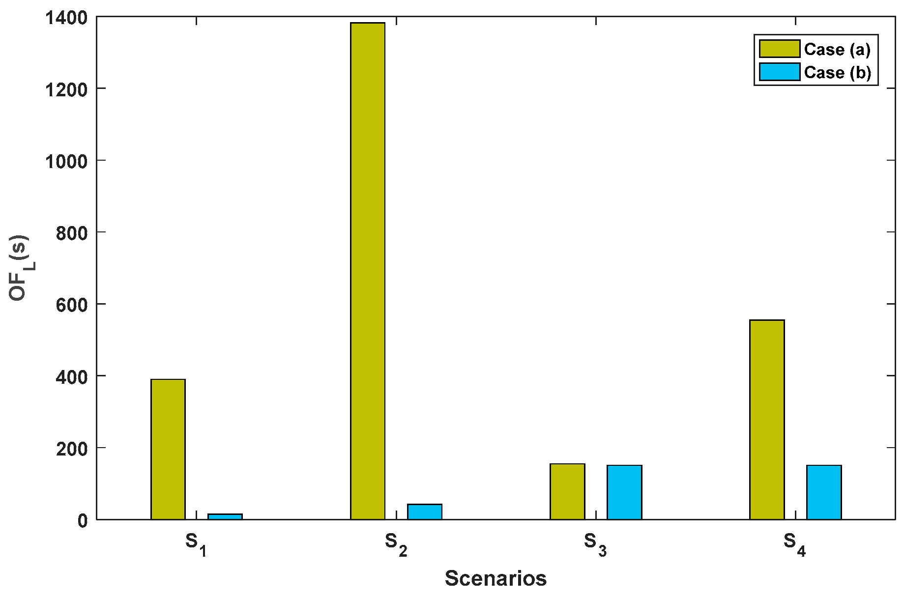
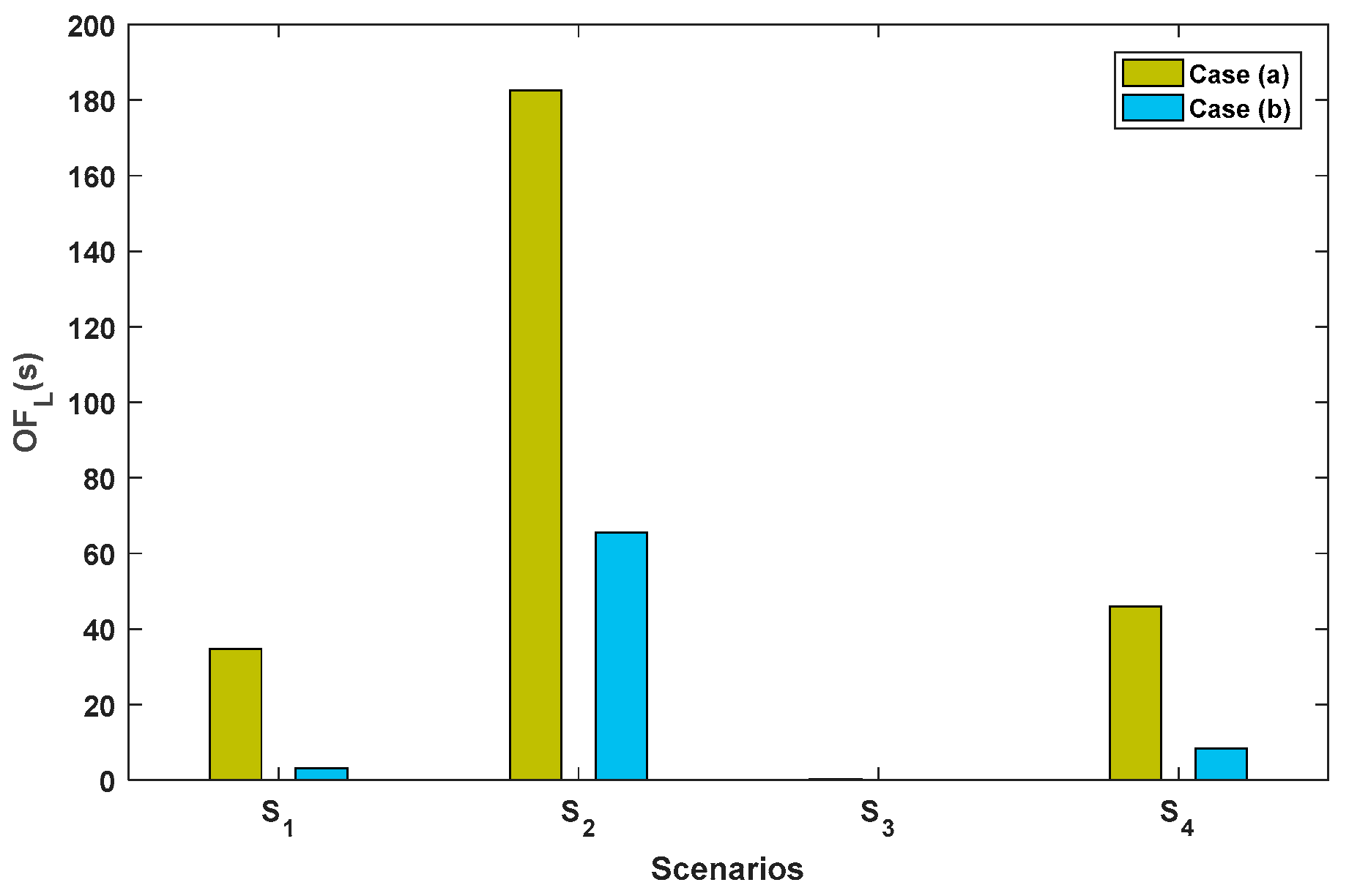
• The lower level’s objective function, i.e., $O{F}_L\left(s\right)$ is the same for scenario 3, where load demand is at its minimum value, and wind intensity is at its maximum.
• The ratio $O{F}_L\left(s\right)$ has the largest difference between cases (a) and (b) in scenario 2, where load demand is at its maximum value, and wind intensity is at its minimum.
• As the load grows, $O{F}_L$ is first reduced in case (a). However, after reaching a particular point in which $O{F}_L$ has its minimum amount, this ratio increases. For a sufficient amount of load growth, $O{F}_L$ would be the same for both cases (a) and (b).

The presented research is limited to the cases where the investor is price taker and there is efficient transmission capacity. In future works, we suggest co-optimizing transmission expansion, energy storage, and wind farm investment, modeling feed-in-tariff and emission cost in the investment problem, and extending the current model to include other sources of renewable energies and the unit commitment-related limitations. Employing AC power flow in the presence of flexible AC transmission system (FACTS) considering reactive power generation capability of wind farms is our focus for future studies.

References

1. IRENA (International Renewable Energy Agency). Wind Energy. 2020. Available online: https://www.irena.org/wind (accessed on 20 June 2023).
2. National Energy Administration. Reports on Wind Power Annual Operation. Available online: http://www.nea.gov.cn/2019-01/28/c_137780779.htm (accessed on 20 June 2023).
3. Xia, F.; Lu, X.; Song, F. The Role of Feed-in Tariff in the Curtailment of Wind Power in China. Energy Econ. 2020, 86, 104661. [Google Scholar] [CrossRef]
4. Baringo, L.; Conejo, A.J. Wind Power Investment within a Market Environment. Appl. Energy 2011, 88, 3239–3247. [Google Scholar] [CrossRef]
5. Baringo, L.; Conejo, A.J. Wind Power Investment: A Benders Decomposition Approach. IEEE Trans. Power Syst. 2012, 27, 433–441. [Google Scholar] [CrossRef]
6. Baringo, L.; Conejo, A.J. Risk-Constrained Multi-Stage Wind Power Investment. IEEE Trans. Power Syst. 2013, 28, 401–411. [Google Scholar] [CrossRef]
7. Li, C.; Lu, G.; Wu, S. The Investment Risk Analysis of Wind Power Project in China. Renew. Energy 2013, 50, 481–487. [Google Scholar] [CrossRef]
8. Baringo, L.; Conejo, A.J. Strategic Wind Power Investment. IEEE Trans. Power Syst. 2014, 29, 1250–1260. [Google Scholar] [CrossRef]
9. Baringo, L.; Conejo, A.J. Transmission and Wind Power Investment. IEEE Trans. Power Syst. 2012, 27, 885–893. [Google Scholar] [CrossRef]
10. Zolfaghari, S.; Akbari, T. Bilevel Transmission Expansion Planning Using Second-Order Cone Programming Considering Wind Investment. Energy 2018, 154, 455–465. [Google Scholar] [CrossRef]
11. Barforoushi, T. Strategic Wind Power Investment in Competitive Electricity Markets Considering the Possibility of Participation in Intraday Market. IET Gener. Transm. Distrib. 2020, 14, 2676–2686. [Google Scholar]
12. Nikkhah, S.; Rabiee, A. Optimal Wind Power Generation Investment, Considering Voltage Stability of Power Systems. Renew. Energy 2018, 115, 308–325. [Google Scholar] [CrossRef]
13. Lam, J.C.K.; Woo, C.K.; Kahrl, F.; Yu, W.K. What Moves Wind Energy Development in China? Show Me the Money! Appl. Energy 2013, 105, 423–429. [Google Scholar] [CrossRef]
14. Hitaj, C.; Löschel, A. The Impact of a Feed-in Tariff on Wind Power Development in Germany. Resour. Energy Econ. 2019, 57, 18–35. [Google Scholar] [CrossRef] [Green Version]
15. Arabpour, A.; Besmi, M.R.; Maghouli, P. Transmission Expansion and Reactive Power Planning Considering Wind Energy Investment Using a Linearized AC Model. J. Electr. Eng. Technol. 2019, 14, 1035–1043. [Google Scholar] [CrossRef]
16. Alishahi, E.; Moghaddam, M.P.; Sheikh-El-Eslami, M.K. A System Dynamics Approach for Investigating Impacts of Incentive Mechanisms on Wind Power Investment. Renew. Energy 2012, 37, 310–317. [Google Scholar] [CrossRef]
17. Li, H.; Qiao, Y.; Lu, Z.; Zhang, B.; Teng, F. Frequency-Constrained Stochastic Planning Towards a High Renewable Target Considering Frequency Response Support from Wind Power. IEEE Trans. Power Syst. 2021, 36, 4632–4644. [Google Scholar] [CrossRef]
18. Ullmark, J.; Göransson, L.; Chen, P.; Bongiorno, M.; Johnsson, F. Inclusion of Frequency Control Constraints in Energy System Investment Modeling. Renew. Energy 2021, 173, 249–262. [Google Scholar] [CrossRef]
19. Gil-González, W.; Montoya, O.D.; Grisales-Noreña, L.F.; Perea-Moreno, A.-J.; Hernandez-Escobedo, Q. Optimal Placement and Sizing of Wind Generators in AC Grids Considering Reactive Power Capability and Wind Speed Curves. Sustainability 2020, 12, 2983. [Google Scholar] [CrossRef] [Green Version]
20. Baringo, L.; Conejo, A.J. Correlated Wind-Power Production and Electric Load Scenarios for Investment Decisions. Appl. Energy 2013, 101, 475–482. [Google Scholar] [CrossRef]
21. Spyridonidou, S.; Vagiona, D.G.; Loukogeorgaki, E. Strategic Planning of Offshore Wind Farms in Greece. Sustainability 2020, 12, 905. [Google Scholar] [CrossRef] [Green Version]
22. Xu, M.; Zhuan, X. Optimal Planning for Wind Power Capacity in an Electric Power System. Renew. Energy 2013, 53, 280–286. [Google Scholar] [CrossRef]
23. Zhao, X.; Yao, J.; Sun, C.; Pan, W. Impacts of Carbon Tax and Tradable Permits on Wind Power Investment in China. Renew. Energy 2019, 135, 1386–1399. [Google Scholar] [CrossRef]
24. Zhu, M.; Qi, Y.; Belis, D.; Lu, J.; Kerremans, B. The China Wind Paradox: The Role of State-Owned Enterprises in Wind Power Investment versus Wind Curtailment. Energy Policy 2019, 127, 200–212. [Google Scholar] [CrossRef]
25. Zhou, Y.; Zhai, Q.; Yuan, W.; Wu, J. Capacity Expansion Planning for Wind Power and Energy Storage Considering Hourly Robust Transmission Constrained Unit Commitment. Appl. Energy 2021, 302, 117570. [Google Scholar] [CrossRef]
26. Ouammi, A.; Dagdougui, H.; Sacile, R. Optimal Planning with Technology Selection for Wind Power Plants in Power Distribution Networks. IEEE Syst. J. 2019, 13, 3059–3069. [Google Scholar] [CrossRef]
27. Ayvaz, A.; Genc, I. A Novel Optimization Method for Wind Power Investment Considering Economic and Security Concerns. J. Renew. Sustain. Energy 2022, 14, 16301. [Google Scholar] [CrossRef]
28. García Mazo, C.M.; Olaya, Y.; Botero Botero, S. Investment in Renewable Energy Considering Game Theory and Wind-Hydro Diversification. Energy Strateg. Rev. 2020, 28, 100447. [Google Scholar] [CrossRef]
29. Alshamrani, A.M.; Alrasheedi, A.F.; Alnowibet, K.A. A Game-Theoretic Model for Wind Farm Planning Problem: A Bi-Level Stochastic Optimization Approach. Sustain. Energy Technol. Assess. 2022, 53, 102539. [Google Scholar] [CrossRef]
30. Aquila, G.; de Queiroz, A.R.; Balestrassi, P.P.; Rotella Junior, P.; Rocha, L.C.S.; Pamplona, E.O.; Nakamura, W.T. Wind Energy Investments Facing Uncertainties in the Brazilian Electricity Spot Market: A Real Options Approach. Sustain. Energy Technol. Assess. 2020, 42, 100876. [Google Scholar] [CrossRef]
31. Liu, Q.; Sun, Y.; Liu, L.; Wu, M. An Uncertainty Analysis for Offshore Wind Power Investment Decisions in the Context of the National Subsidy Retraction in China: A Real Options Approach. J. Clean. Prod. 2021, 329, 129559. [Google Scholar] [CrossRef]
32. Xu, G.; Cheng, H.; Fang, S.; Ma, Z.; Zeng, P.; Yao, L. Optimal Size and Location of Battery Energy Storage Systems for Reducing the Wind Power Curtailments. Electr. Power Compon. Syst. 2018, 46, 342–352. [Google Scholar] [CrossRef]
33. Neto, D.P.; Domingues, E.G.; Calixto, W.P.; Alves, A.J. Methodology of Investment Risk Analysis for Wind Power Plants in the Brazilian Free Market. Electr. Power Compon. Syst. 2018, 46, 316–330. [Google Scholar] [CrossRef]
34. Zeng, B.; Zhang, J.; Ouyang, S.; Yang, X.; Dong, J.; Zeng, M. Two-Stage Combinatory Planning Method for Efficient Wind Power Integration in Smart Distribution Systems Considering Uncertainties. Electr. Power Compon. Syst. 2014, 42, 1661–1672. [Google Scholar] [CrossRef]
35. Liu, Q.; Sun, Y.; Wu, M. Decision-Making Methodologies in Offshore Wind Power Investments: A Review. J. Clean. Prod. 2021, 295, 126459. [Google Scholar] [CrossRef]
36. Huang, S.; Suo, C.; Guo, J.; Lv, J.; Jing, R.; Yu, L.; Fan, Y.; Ding, Y. Balancing the Water-Energy Dilemma in Nexus System Planning with Bi-Level and Multi-Uncertainty. Energy 2023, 278, 127720. [Google Scholar] [CrossRef]
37. Yang, J.; Shi, X.; Prokopyev, O.A. Exact Solution Approaches for a Class of Bilevel Fractional Programs. Optim. Lett. 2022, 17, 191–210. [Google Scholar] [CrossRef]
38. Radzik, T. Fractional Combinatorial Optimization. In Handbook of Combinatorial Optimization; Springer: Berlin/Heidelberg, Germany, 1998; pp. 429–478. [Google Scholar]
39. Borrero, J.S.; Gillen, C.; Prokopyev, O.A. Fractional 0–1 Programming: Applications and Algorithms. J. Glob. Optim. 2017, 69, 255–282. [Google Scholar] [CrossRef]
40. Dinkelbach, W. On Nonlinear Fractional Programming. Manag. Sci. 1967, 13, 492–498. [Google Scholar] [CrossRef]
41. A Guide for GAMS software, G.U.; GAMS Development Corporation: Washington, DC, USA, 2014.
42. Gurobi Optimization, “Gurobi Optimizer Reference Manual”. Available online: http://www.gurobi.com (accessed on 20 June 2023).