
Energy Efficiency and Optimization Strategies in a Building to Minimize Airborne Infection Risks


Abstract
:1. Introduction
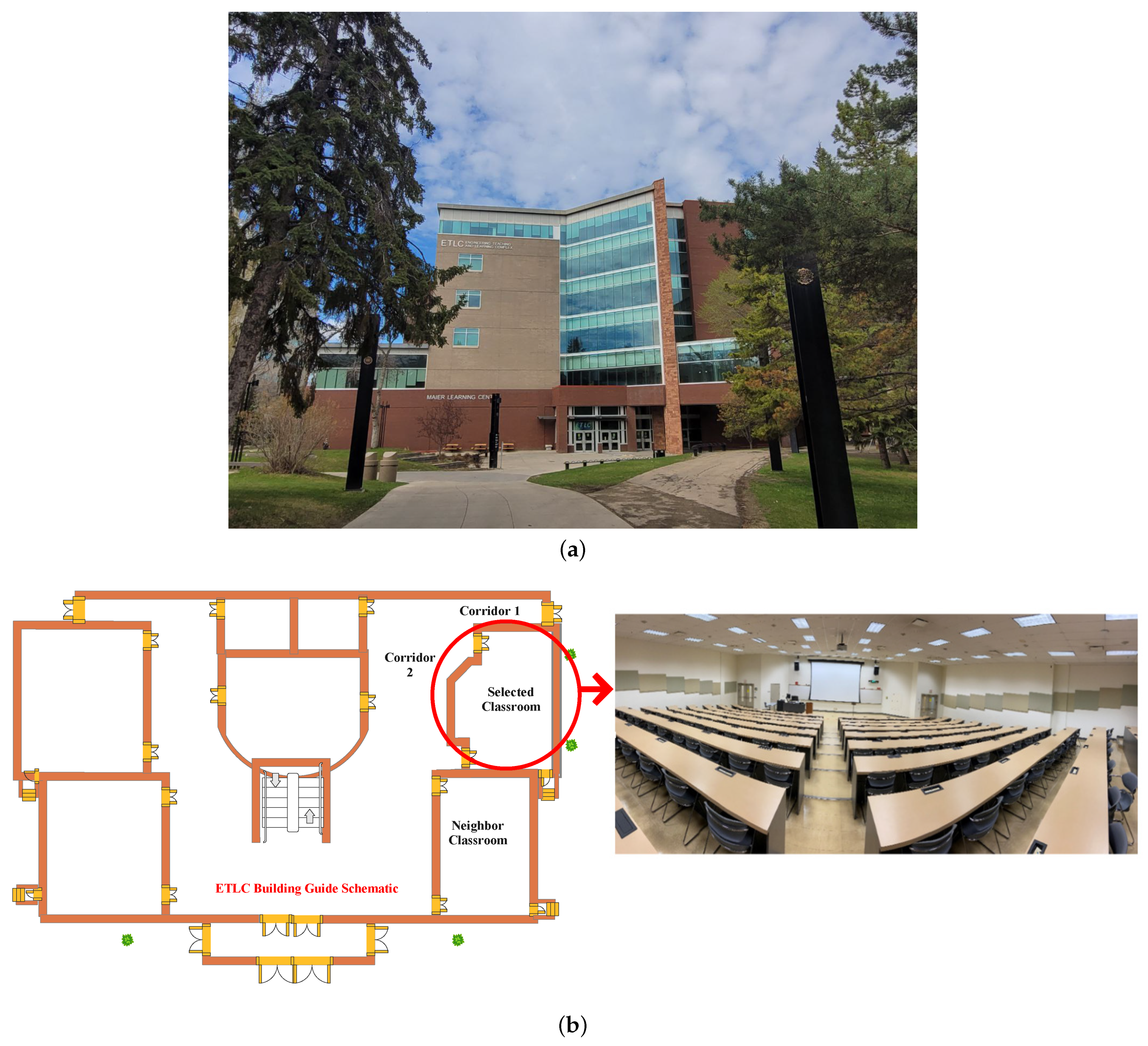
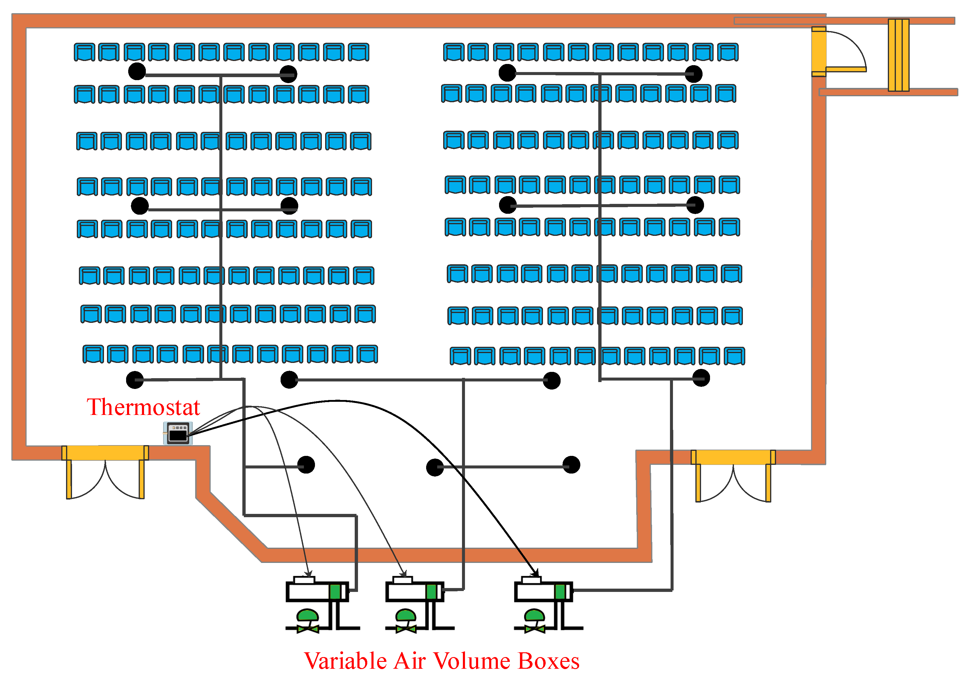
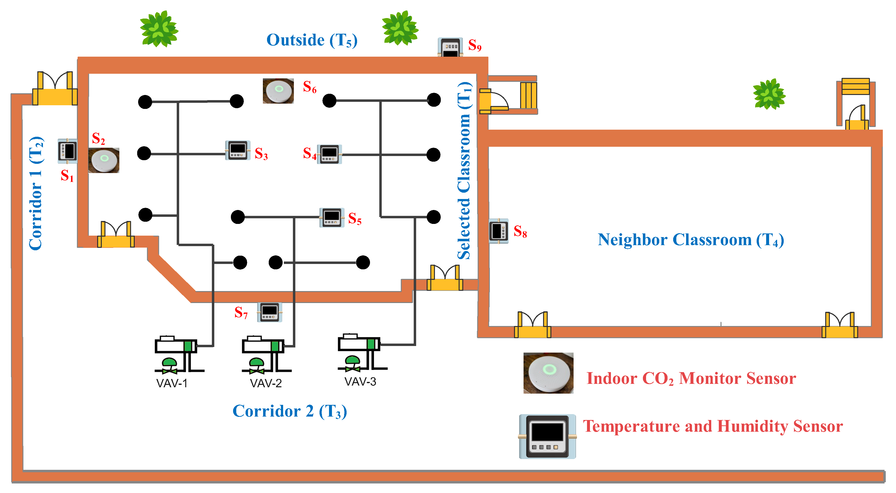
2. Test Setup
3. Plant Models for Use in Controller
3.1. Dynamic Model of Airborne COVID-19 Transmission Risk
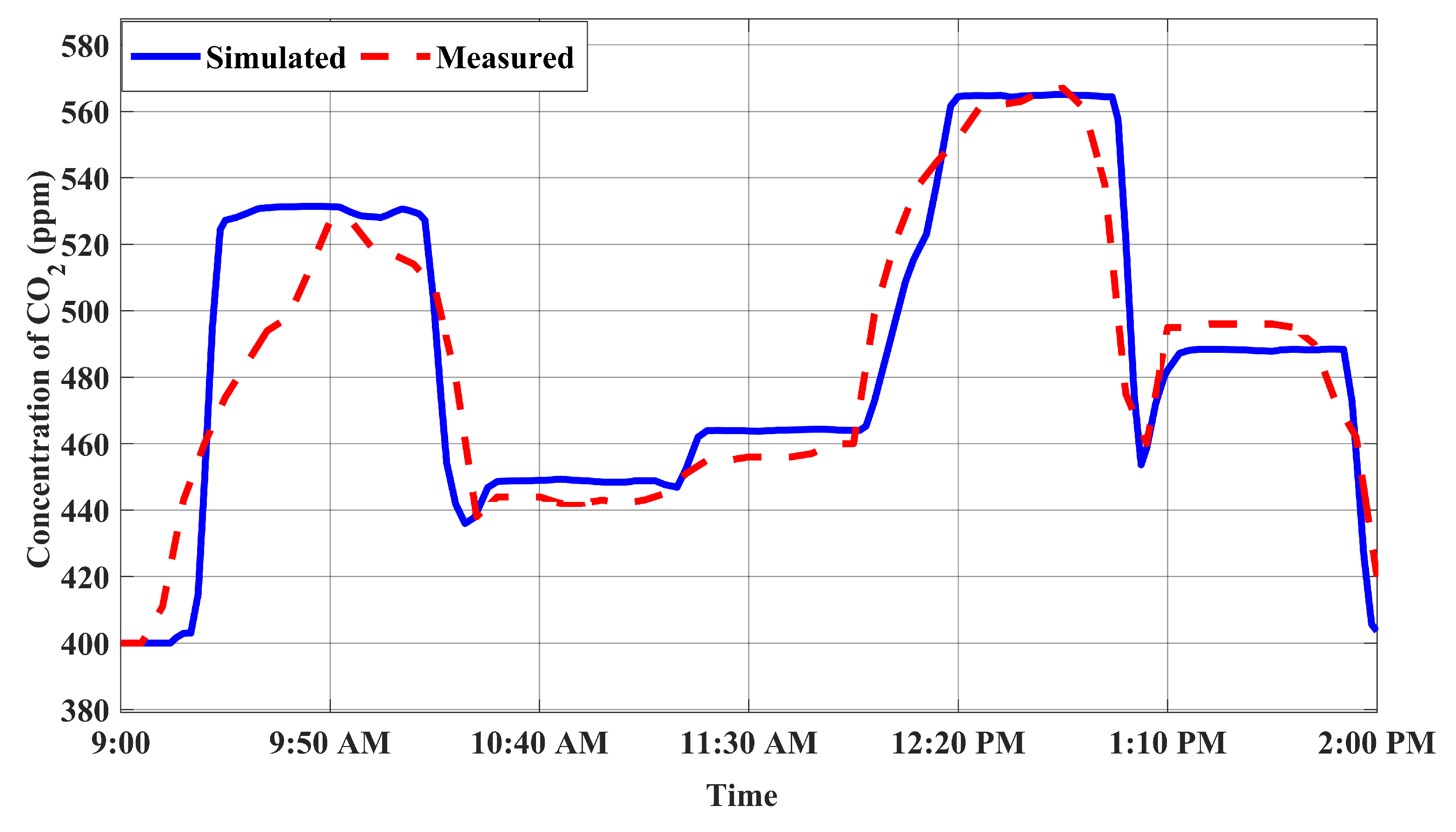
3.2. Concentration Model
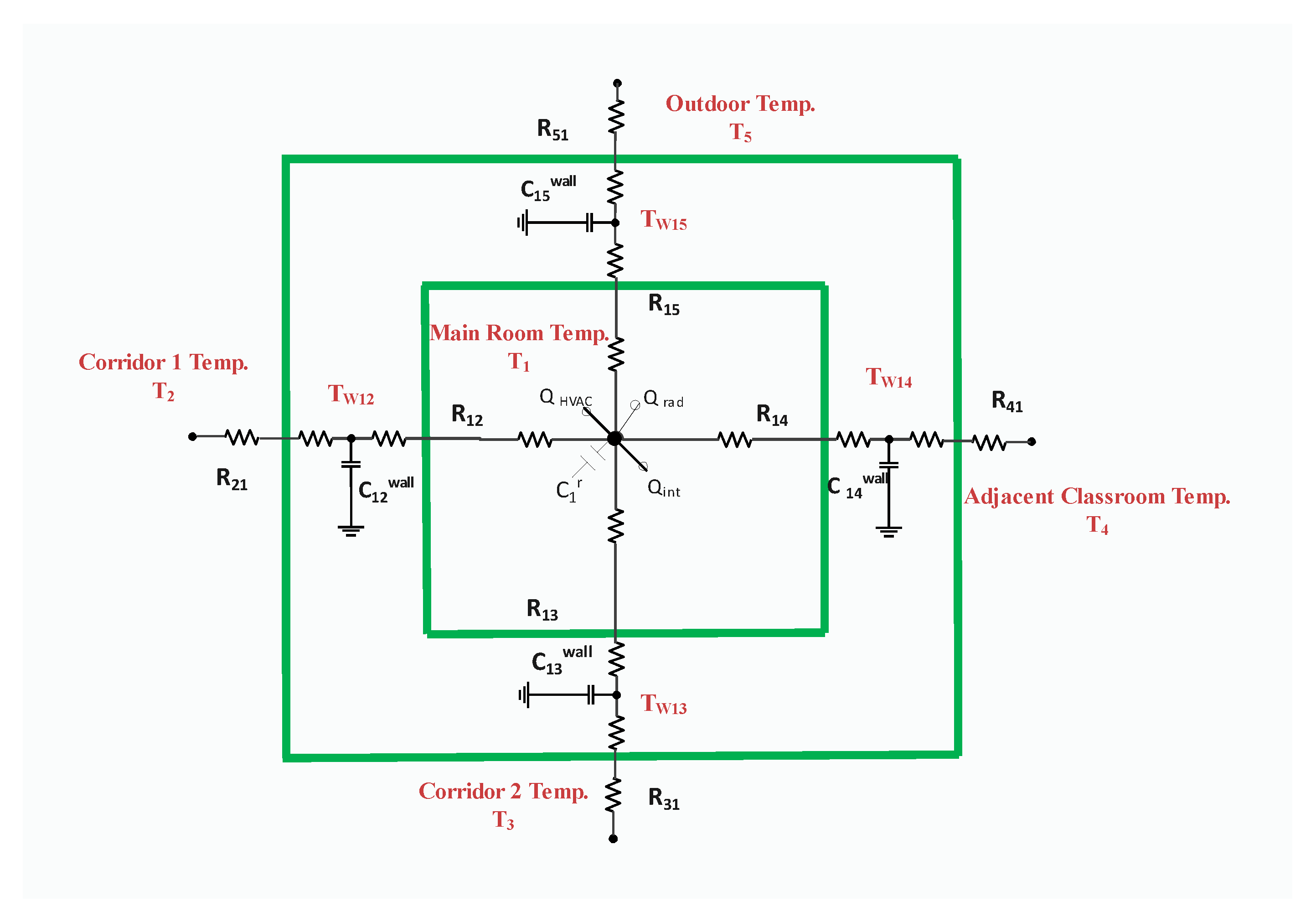
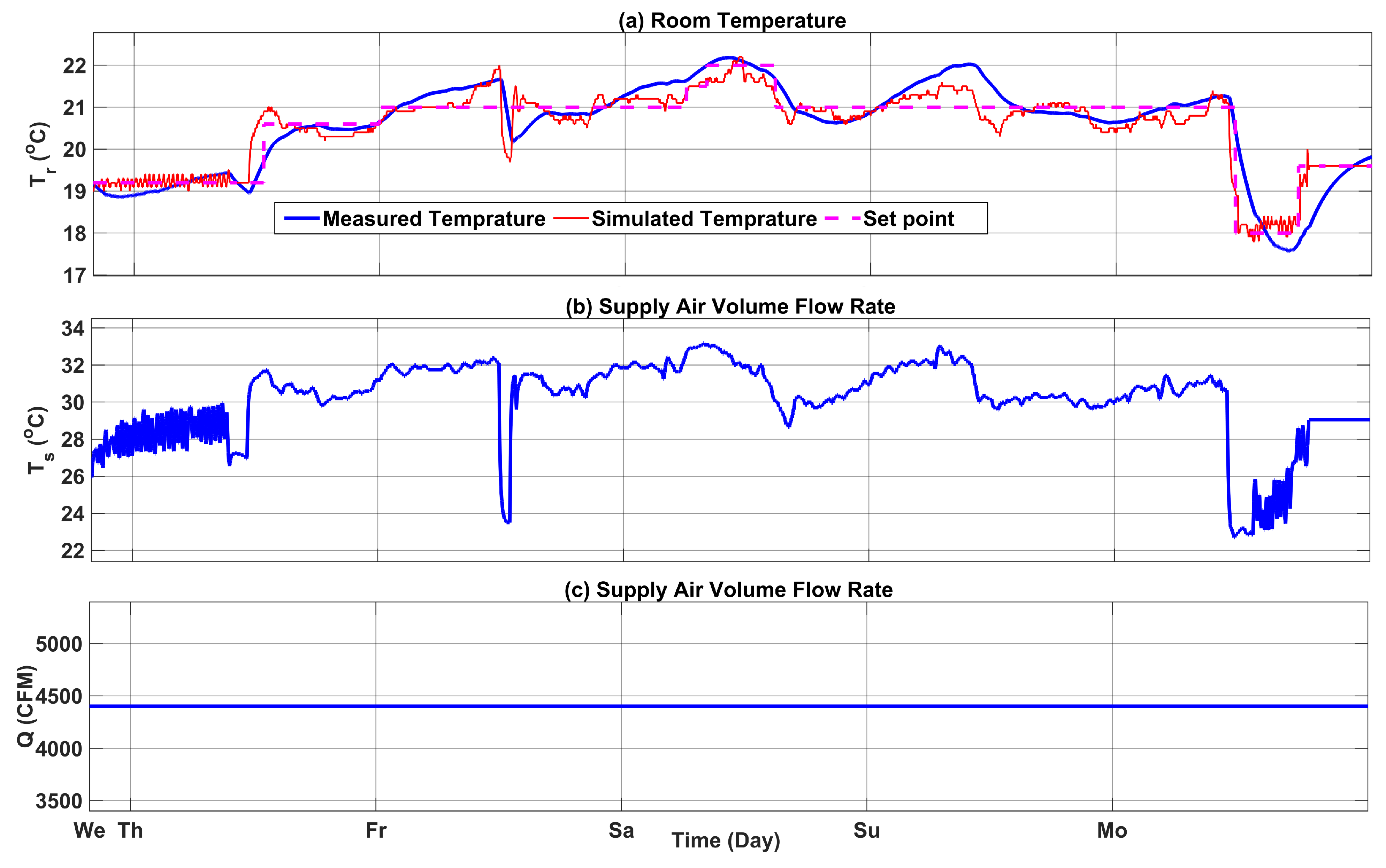
3.3. Building Thermal Model
- Air in the classroom is thoroughly mixed. Thus, the classroom’s temperature and air density are constant across the classroom;
- As the classroom does not have any windows, the effect of solar radiation is negligible;
- Specific heat capacity of air, is equal to 1.007 at 300 ;
- All internal walls have the same properties such as , L, and h.
3.4. State Space Models
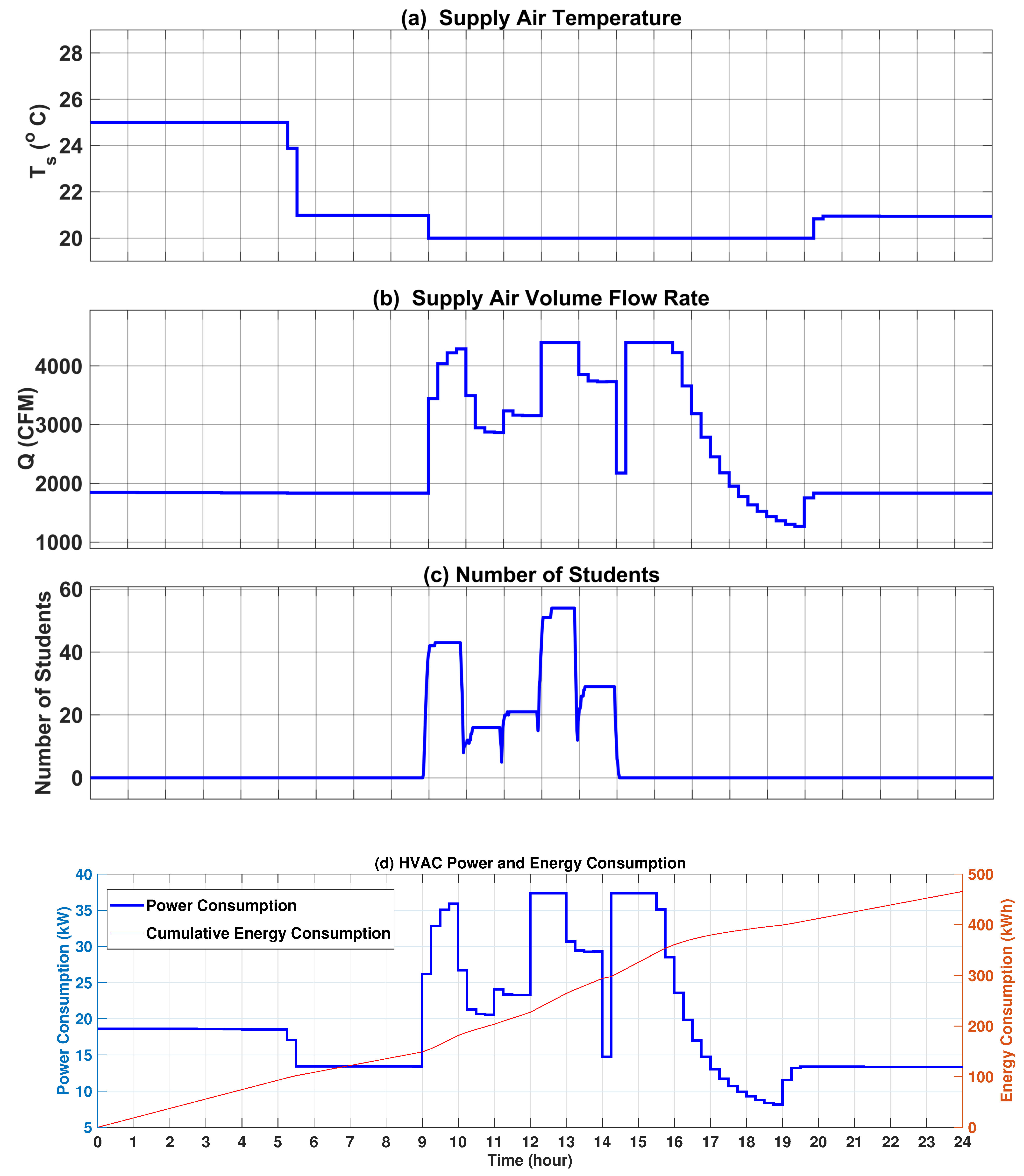
3.5. HVAC Energy Consumption
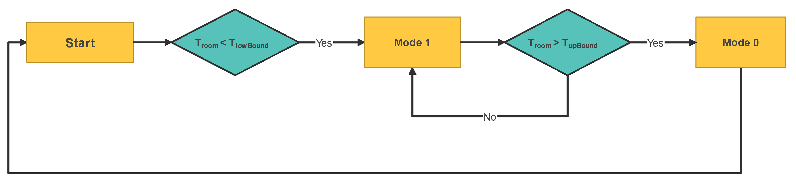
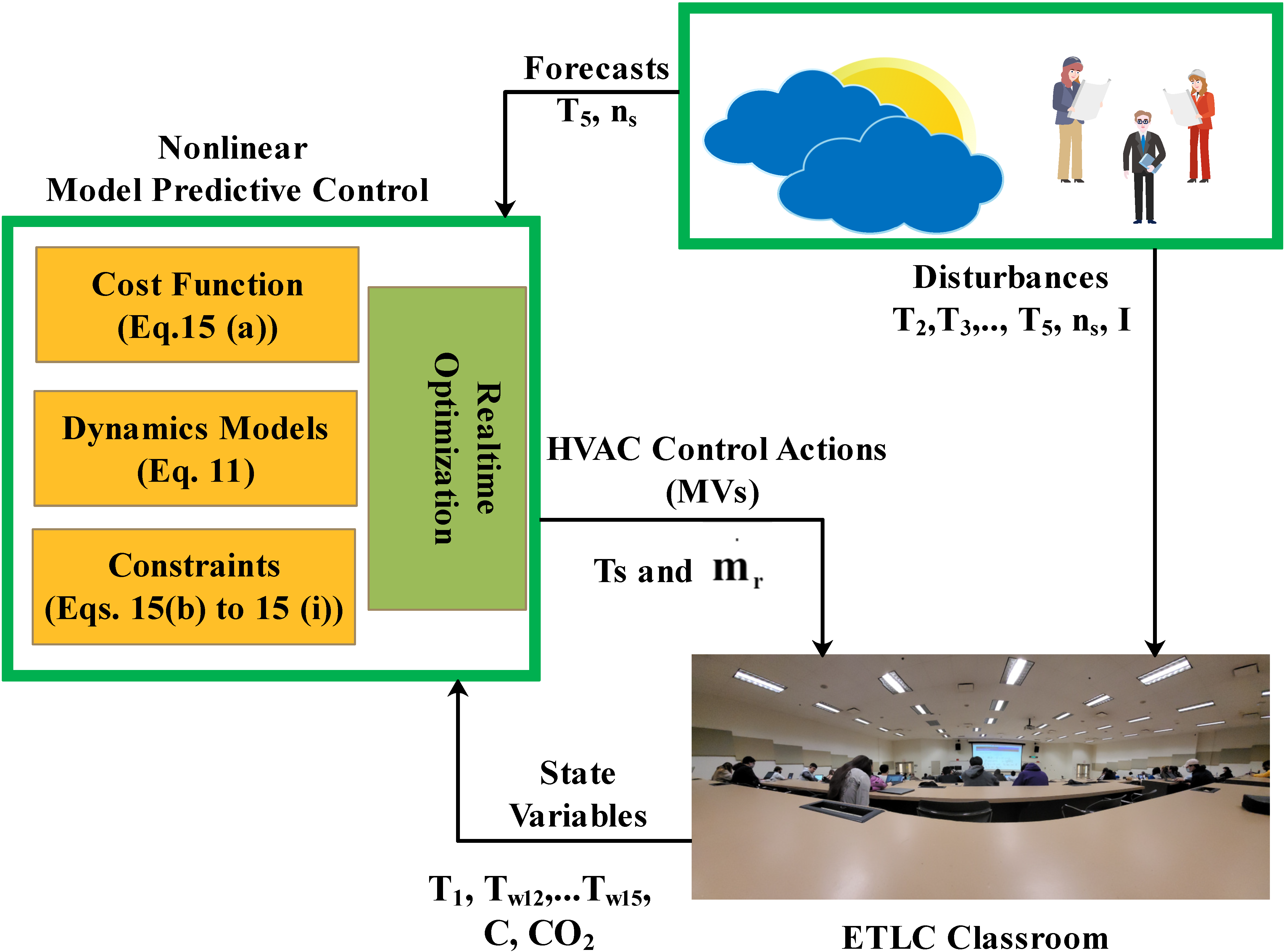
4. Controller Design
- Cost Function: The cost (objective) function in the designed NMPC in this work should be represented by formulations that lead to minimum HVAC energy consumption and minimize the COVID transmission risk. There are different forms of cost functions such as terminal control, minimum control effort, trajectory tracking, minimizing energy consumption, or a combination of them [18]. The cost function in this paper is presented by Equation (15) that includes a combination of minimizing HVAC energy use, minimum control efforts, and trajectory tracking.
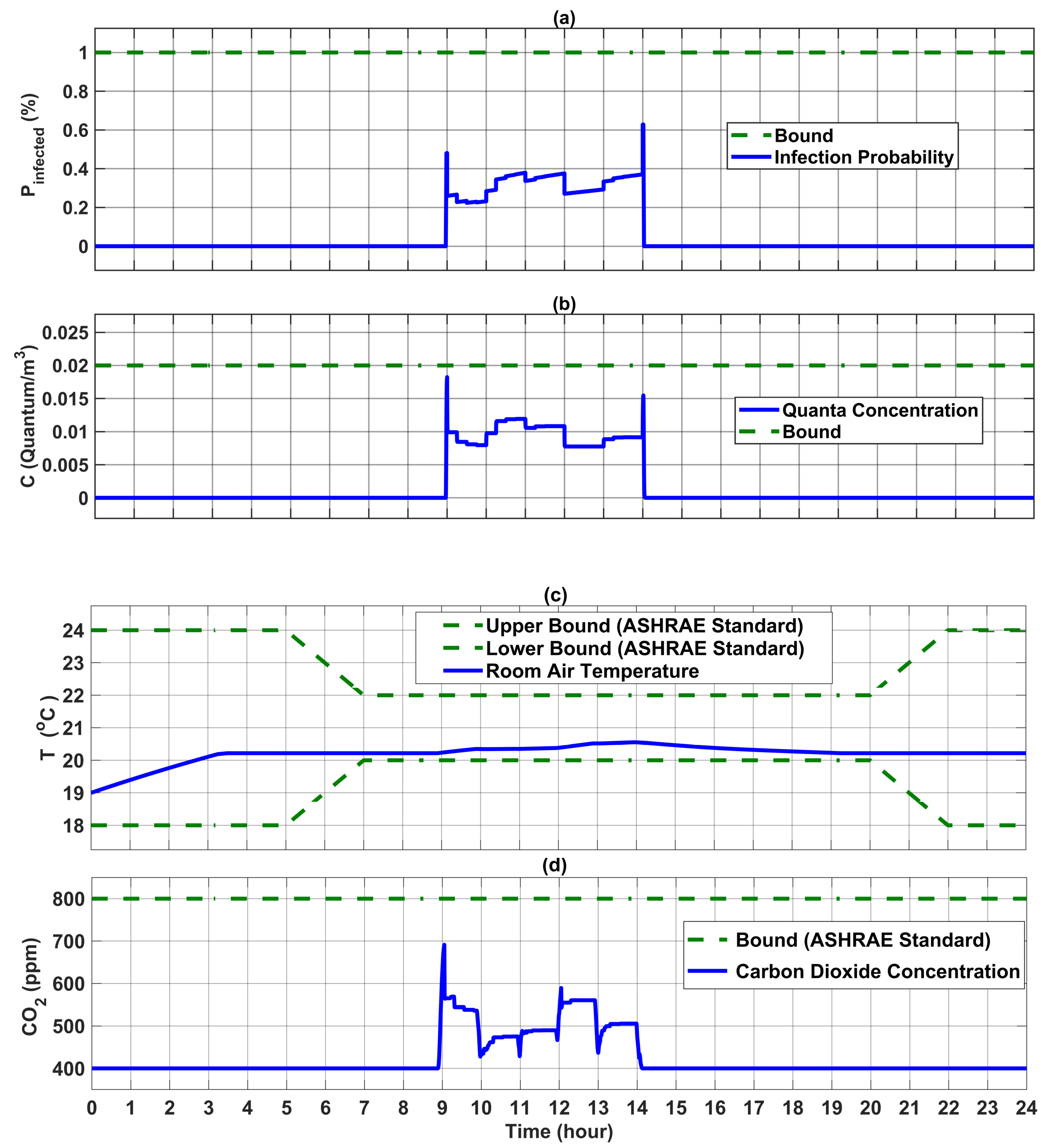
- Constraints: Constraints can be defined as rate or range limits, such as upper and lower bounds of zone temperature or maximum and minimum limits of supply airflow rate [18]. In this paper, inequality constraints are included to enforce (i) low risk of COVID transmission, (ii) meeting ASHRAE comfort level for occupants in terms of room temperature, (iii) minimum ventilation requirement set by level in the room, and iv) control actuators operational constraints (i.e., AHU flow rate, supply air temperature).
- Prediction Horizon, Control Horizon, and Control Time Step: The control horizon is often selected to be less than the prediction horizon to minimize computation cost [18]. In this paper, the sample time, is chosen as 15 min by considering slow room temperature dynamics; the prediction horizon, is 96, which provides the prediction time of 1440 min or 24 h; the control horizon, is chosen as 19.
- Optimizer: Selection of an appropriate optimizer for an NMPC is critical to ensure that a feasible optimal solution can be found in real-time within each control time step. The HVAC control problem in this work includes nonlinear programming (NLP) consisting of a quadratic cost function. Some of the methods to solve NLP problems include active set (AS) methods, first order methods (FOM), interior point (IP) methods, and sequential quadratic programming (SQP) methods [43]. In this work, the SQP algorithm is implemented in Matlab to find feasible solution at each control time step.
5. Results and Discussions
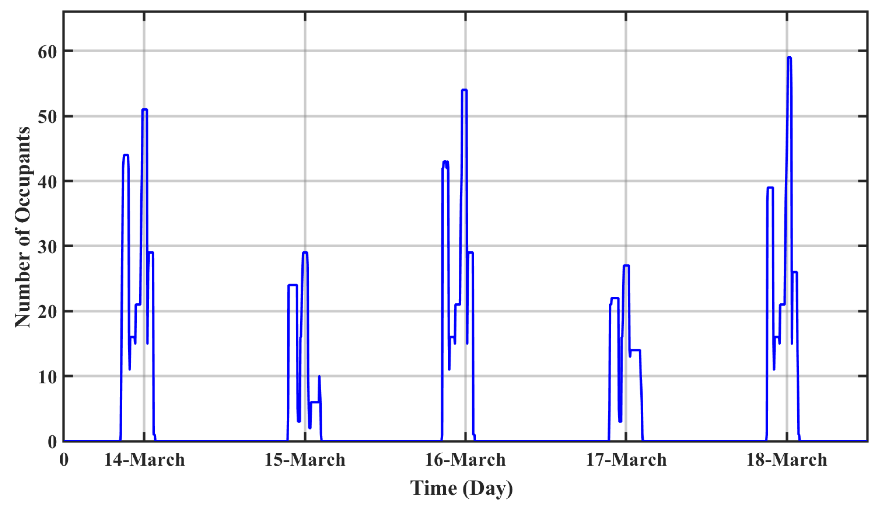
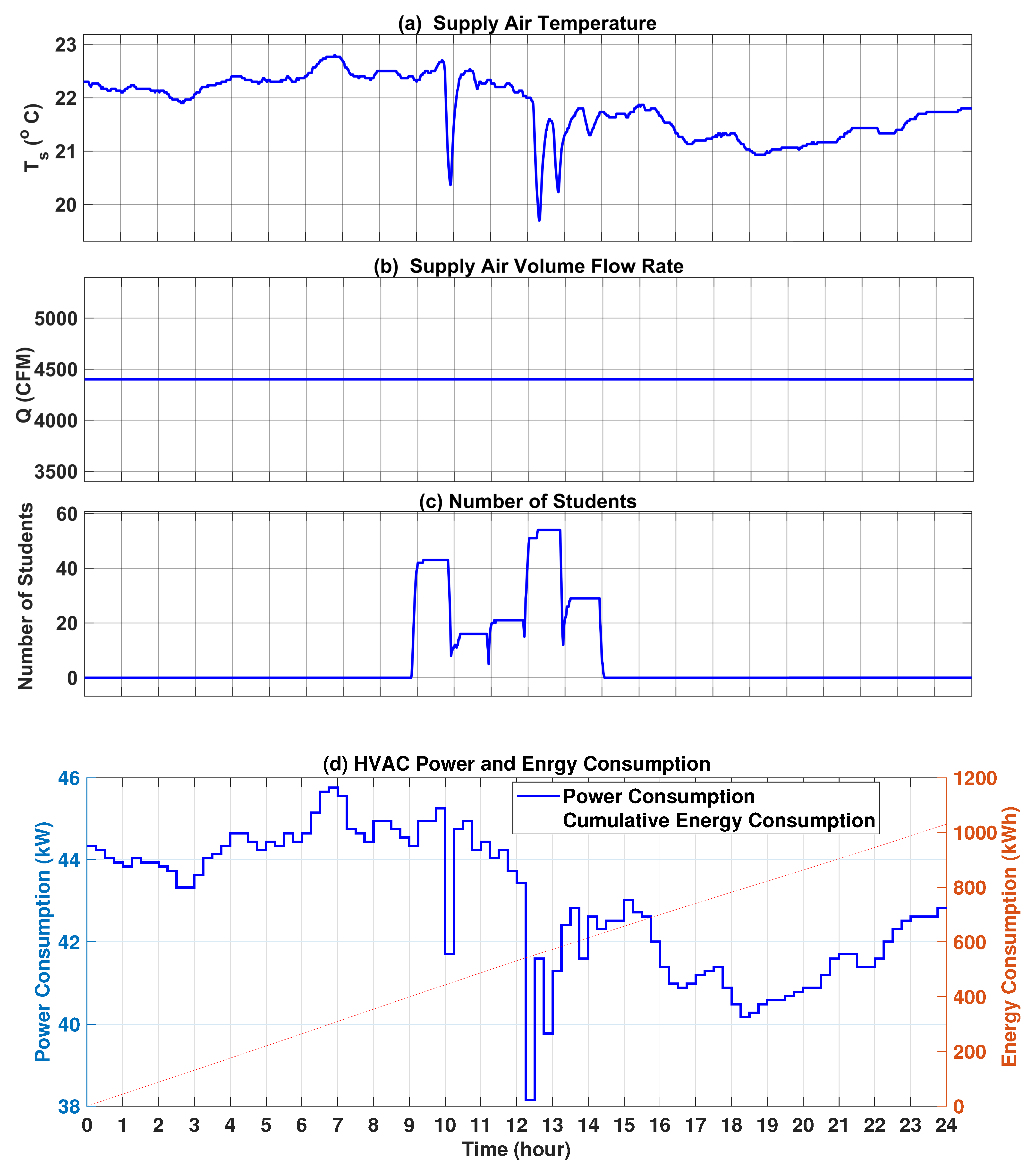
5.1. Experimental Data
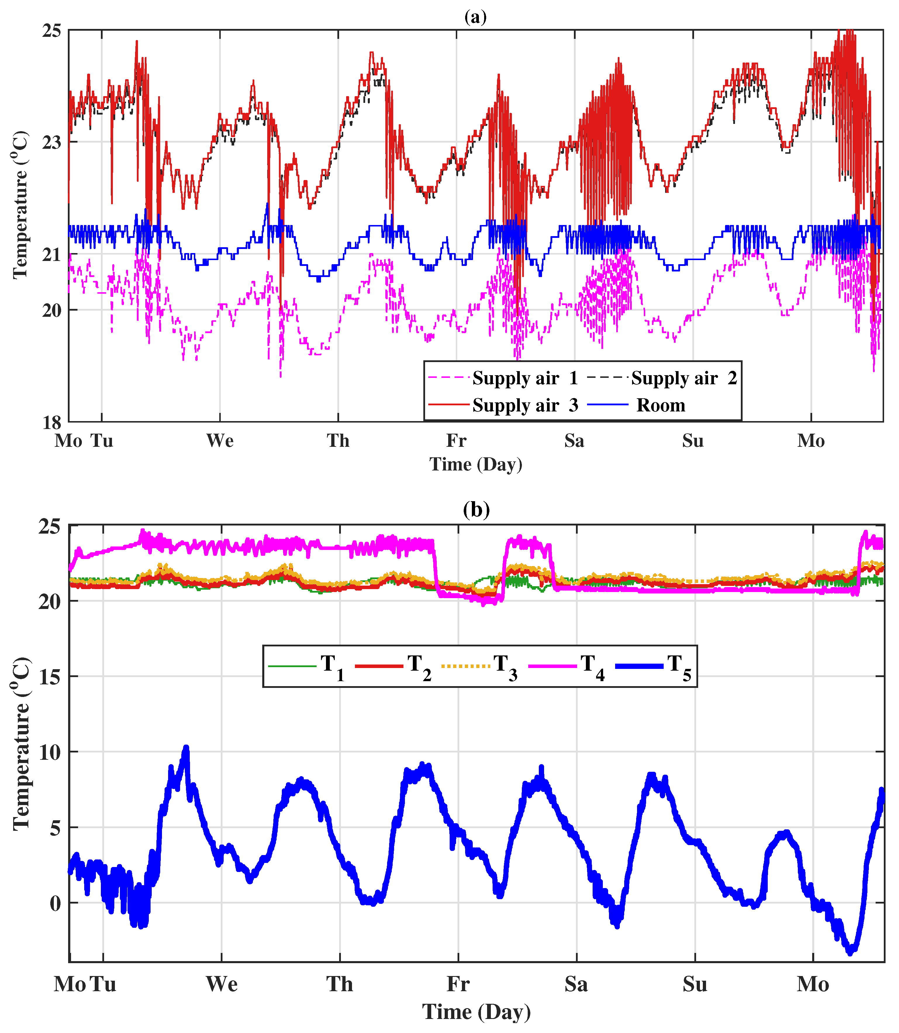
5.2. Model Validation
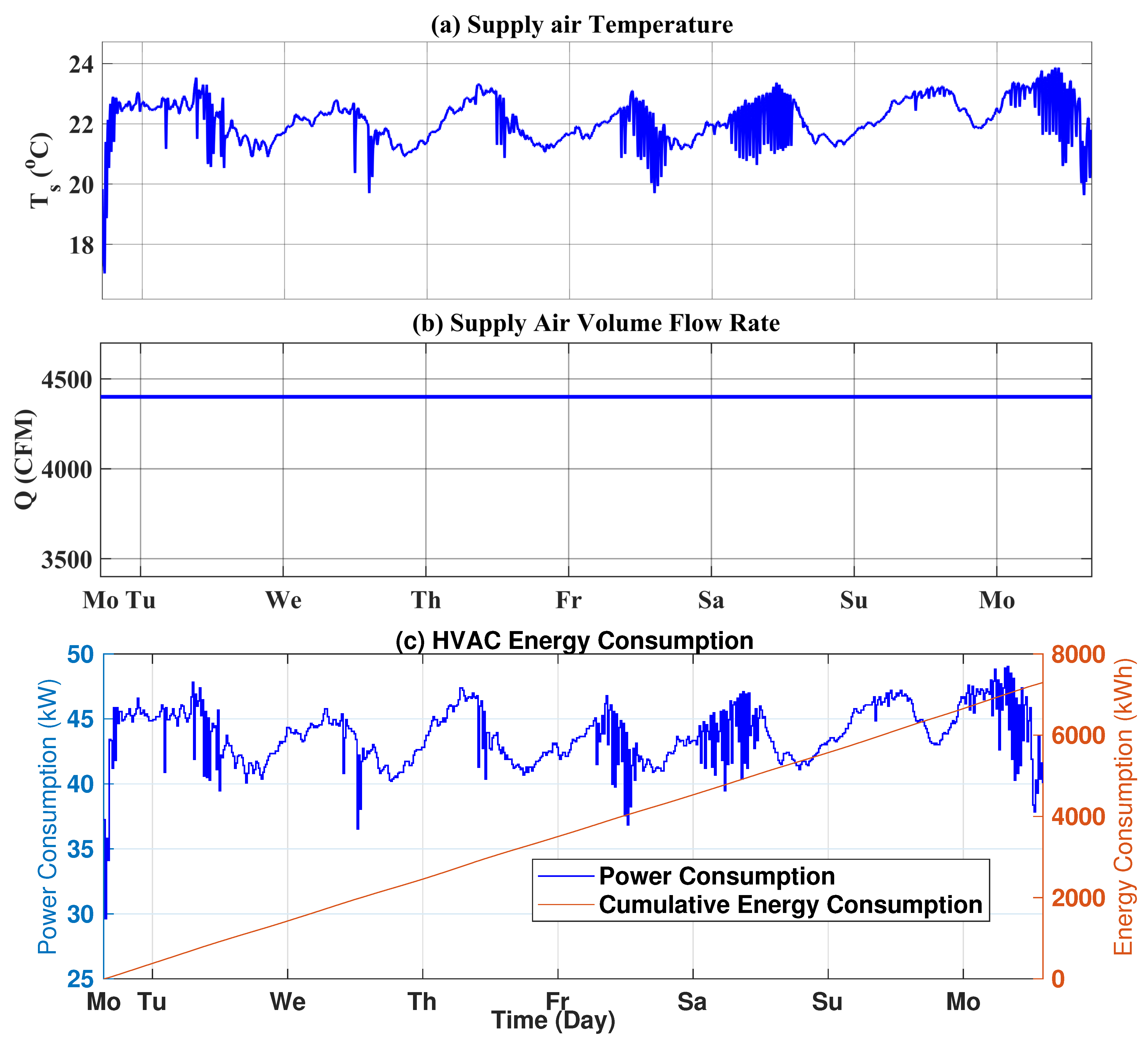
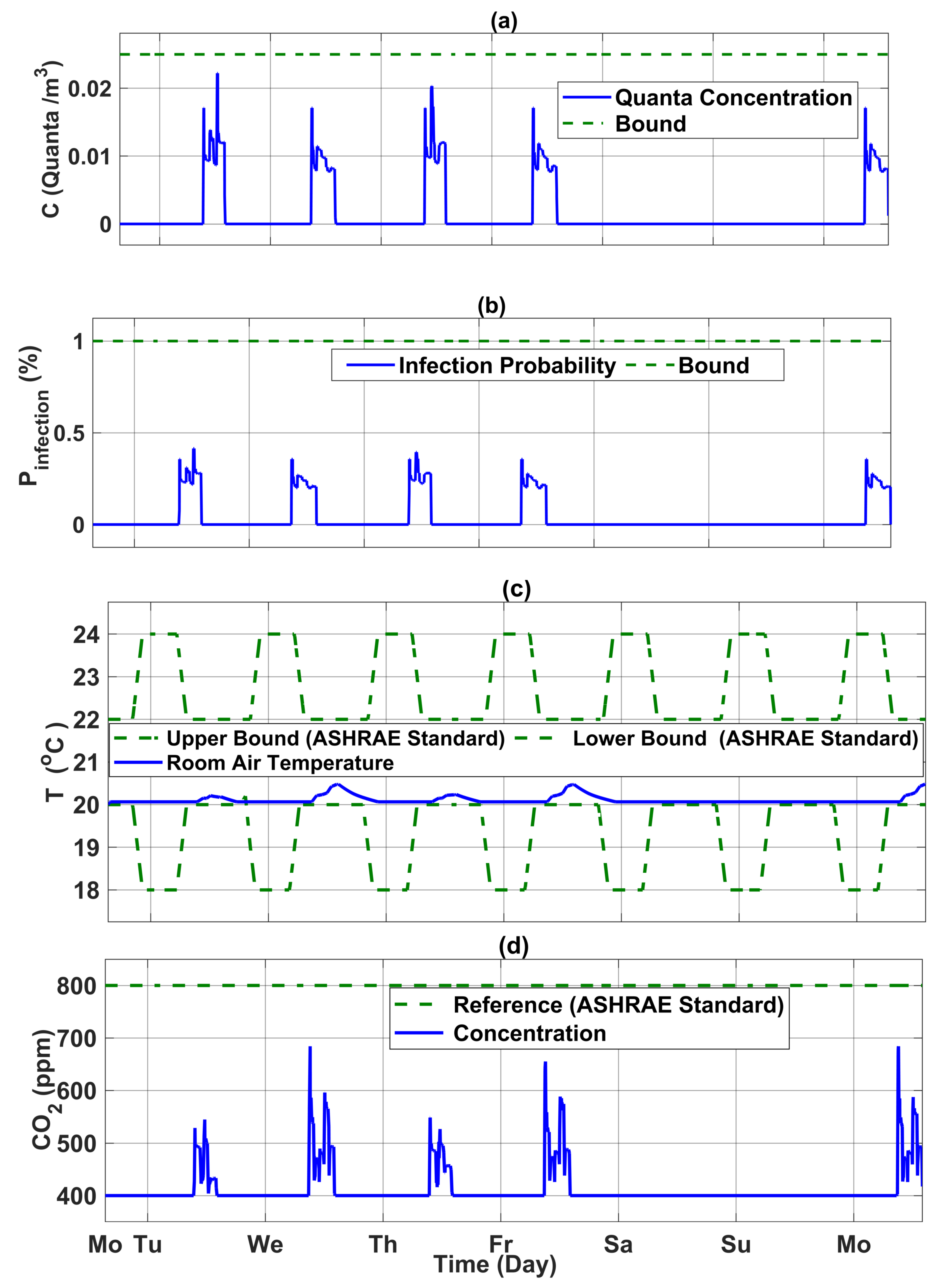
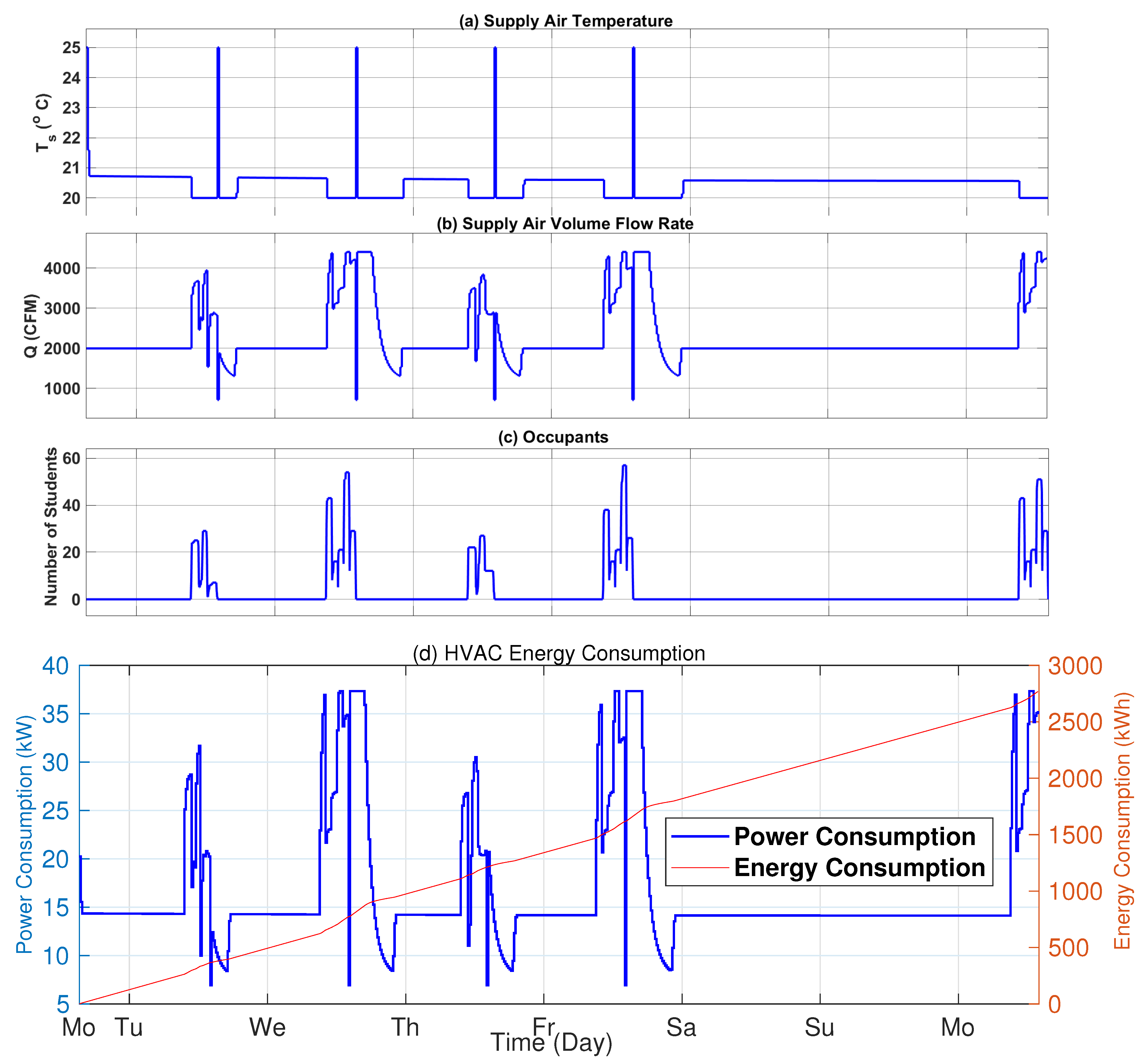
5.3. Control Results
6. Summary and Conclusions
Author Contributions
Funding
Data Availability Statement
Conflicts of Interest
Abbreviations and Nomenclature
| ACH | Air Change Per Hour |
| AHU | Air Handling Unit |
| ASHRAE | American Society of Heating, Refrigerating and Air-Conditioning Engineers |
| COVID-19 | Coronavirus |
| ETLC | Engineering Teaching and Learning Complex |
| H1N1 | Influenza |
| HVAC | Heating, Ventilation, and Air Conditioning |
| IAQ | Indoor Air Quality |
| IMC | Internal Model Controller |
| MD | Measurement Disturbance |
| MERS | Middle East Respiratory Syndrome |
| MPC | Model Predictive Control |
| MV | Manipulated Variable |
| NLP | Nonlinear Programming Problem |
| NMPC | Nonlinear Model Predictive Control |
| PAR | Peak to Average Ratio |
| PI | Proportional-Integral |
| PID | Proportional–Integral–Derivative |
| PM | Particulate Matter |
| PPM | Parts Per Million |
| RBC | Rule-based Control |
| RC | Resistance-Capacitance |
| SARS | Severe Acute Respiratory Syndrome |
| SBMPC | Stochastic Scenario-Based MPC |
| SQP | Sequential Quadratic Programming |
| VAV | Variable Air Volume |
| WHO | World Health Organization |
| Symbols | |
| Prevalence rate of disease (-) | |
| Absorption coefficient of the wall between room i, j (-) | |
| Fan power coefficient (-) | |
| Slack variable | |
| Efficiency of the boilers (-) | |
| Thermal conductivity () | |
| Air change per hour () | |
| Air mass flow rate () | |
| Heat transfer rate (W) | |
| Temperature gradient () | |
| Constant pressure specific heat () | |
| Heat storage capacity () | |
| Stefan-Boltzmann constant () | |
| Duration of event ( | |
| Quanta emission rate (quanta/h) | |
| emission rate of indoor source (mg/s) | |
| Fraction of unreported COVID-19 cases | |
| Generation rate by occupants () | |
| Energy consumption | |
| Conductivity of walls () | |
| Control horizon | |
| Prediction horizon | |
| Daily new COVID-19 cases | |
| Power consumption by fans ( | |
| Power consumption by heating coils ( | |
| Probability of being infected (%) | |
| Volumetric breathing rate of an occupant () | |
| Internal thermal resistance of walls ( | |
| Thermal resistance of outside wall ( | |
| Time step (min) | |
| Temperature () | |
| Velocity (m/s) | |
| Constraint violation penalty weight | |
| Density of air () | |
| Q | Air volume flow rate () |
| Wall density () | |
| Area of walls () | |
| Heat storage capacity of the room () | |
| Heat storage capacity of walls () | |
| Convection heat-transfer coefficient () | |
| Number of infected people (-) | |
| Thickness of wall () | |
| Mass () | |
| Number of students (-) | |
| Volume of the classroom () | |
| Wall volume () |
References
- Falode, A.J.; Bolarinwa, J.O.; Yakubu, M. History of pandemics in the twentieth and twenty-first century. Synesis J. Humanit. Soc. Sci. 2021, 2, 9–26. [Google Scholar] [CrossRef]
- Greenhalgh, T.; Jimenez, J.L.; Prather, K.A.; Tufekci, Z.; Fisman, D.; Schooley, R. Ten scientific reasons in support of the airborne transmission of SARS-CoV-2. Lancet 2021, 397, 1603–1605. [Google Scholar] [CrossRef] [PubMed]
- Prather, K.A.; Marr, L.C.; Schooley, R.T.; McDiarmid, M.A.; Wilson, M.E.; Milton, D.K. Airborne transmission of SARS-CoV-2. Science 2020, 370, 303–304. [Google Scholar] [CrossRef] [PubMed]
- Noorimotlagh, Z.; Jaafarzadeh, N.; Martínez, S.S.; Mirzaee, S.A. A systematic review of possible airborne transmission of the COVID-19 virus (SARS-CoV-2) in the indoor air environment. Environ. Res. 2021, 193, 110612. [Google Scholar] [CrossRef]
- Chu, D.K.; Akl, E.A.; Duda, S.; Solo, K.; Yaacoub, S.; Schünemann, H.J. Physical distancing, face masks, and eye protection to prevent person-to-person transmission of SARS-CoV-2 and COVID-19: A systematic review and meta-analysis. Lancet 2020, 395, 1973–1987. [Google Scholar] [CrossRef]
- Azimi, P.; Stephens, B. HVAC filtration for controlling infectious airborne disease transmission in indoor environments: Predicting risk reductions and operational costs. Build. Environ. 2013, 70, 150–160. [Google Scholar] [CrossRef]
- Thuresson, S.; Fraenkel, C.J.; Sasinovich, S.; Soldemyr, J.; Widell, A.; Medstrand, P.; Alsved, M.; Löndahl, J. Airborne severe acute respiratory syndrome coronavirus 2 (SARS-CoV-2) in hospitals: Effects of aerosol-generating procedures, HEPA-filtration units, patient viral load, and physical distance. Clin. Infect. Dis. 2022, 75, e89–e96. [Google Scholar] [CrossRef]
- Feng, Z.; Cao, S.J.; Haghighat, F. Removal of SARS-CoV-2 using UV+ Filter in built environment. Sustain. Cities Soc. 2021, 74, 103226. [Google Scholar] [CrossRef]
- Yang, Y.; Zhang, H.; Chan, V.; Lai, A.C. Development and experimental validation of a mathematical model for the irradiance of in-duct ultraviolet germicidal lamps. Build. Environ. 2019, 152, 160–171. [Google Scholar] [CrossRef]
- Yang, Y.; Zhang, H.; Nunayon, S.S.; Chan, V.; Lai, A.C. Disinfection efficacy of ultraviolet germicidal irradiation on airborne bacteria in ventilation ducts. Indoor Air 2018, 28, 806–817. [Google Scholar] [CrossRef] [PubMed]
- Qian, H.; Zheng, X. Ventilation control for airborne transmission of human exhaled bio-aerosols in buildings. J. Thorac. Dis. 2018, 10, S2295. [Google Scholar] [CrossRef]
- Qian, H.; Li, Y. Removal of exhaled particles by ventilation and deposition in a multibed airborne infection isolation room. Indoor Air 2010, 20, 284–297. [Google Scholar] [CrossRef]
- Razmara, M.; Maasoumy, M.; Shahbakhti, M.; Robinett, R., III. Optimal exergy control of building HVAC system. Appl. Energy 2015, 156, 555–565. [Google Scholar] [CrossRef]
- Razmara, M.; Maasoumy, M.; Shahbakhti, M.; Robinett, R.D. Exergy-based model predictive control for building HVAC systems. In Proceedings of the 2015 American Control Conference (ACC), Chicago, IL, USA, 1–3 July 2015; IEEE: Piscataway, NJ, USA, 2015; pp. 1677–1682. [Google Scholar]
- Pérez-Lombard, L.; Ortiz, J.; Pout, C. A review on buildings energy consumption information. Energy Build. 2008, 40, 394–398. [Google Scholar] [CrossRef]
- Harrold, M.; Lush, D. Automatic controls in building services. In Proceedings of the IEE Proceedings B (Electric Power Applications); IET: Rochester, NY, USA, 1988; Volume 135, pp. 105–133. [Google Scholar] [CrossRef]
- Al-Rabghi, O.M.; Akyurt, M.M. A survey of energy-efficient strategies for effective air conditioning. Energy Convers. Manag. 2004, 45, 1643–1654. [Google Scholar] [CrossRef]
- Afram, A.; Janabi-Sharifi, F. Theory and applications of HVAC control systems—A review of model predictive control (MPC). Build. Environ. 2014, 72, 343–355. [Google Scholar] [CrossRef]
- Arguello-Serrano, B.; Velez-Reyes, M. Nonlinear control of a heating, ventilating, and air conditioning system with thermal load estimation. IEEE Trans. Control Syst. Technol. 1999, 7, 56–63. [Google Scholar] [CrossRef]
- Wang, J.; Huang, J.; Feng, Z.; Cao, S.J.; Haghighat, F. Occupant-density-detection based energy efficient ventilation system: Prevention of infection transmission. Energy Build. 2021, 240, 110883. [Google Scholar] [CrossRef]
- Walker, S.S.; Lombardi, W.; Lesecq, S.; Roshany-Yamchi, S. Application of distributed model predictive approaches to temperature and CO2 concentration control in buildings. IFAC—PapersOnLine 2017, 50, 2589–2594. [Google Scholar] [CrossRef]
- Maasoumy, M.; Sangiovanni-Vincentelli, A. Total and peak energy consumption minimization of building HVAC systems using model predictive control. IEEE Des. Test Comput. 2012, 29, 26–35. [Google Scholar] [CrossRef] [Green Version]
- Vašak, M.; Starčić, A.; Martinčević, A. Model predictive control of heating and cooling in a family house. In Proceedings of the 2011 Proceedings of the 34th International Convention MIPRO, Opatija, Croatia, 23–27 May 2011; IEEE: Piscataway, NJ, USA, 2011; pp. 739–743. [Google Scholar]
- Pippia, T.; Lago, J.; De Coninck, R.; De Schutter, B. Scenario-based nonlinear model predictive control for building heating systems. Energy Build. 2021, 247, 111108. [Google Scholar] [CrossRef]
- Ganesh, H.S.; Fritz, H.E.; Edgar, T.F.; Novoselac, A.; Baldea, M. A model-based dynamic optimization strategy for control of indoor air pollutants. Energy Build. 2019, 195, 168–179. [Google Scholar] [CrossRef]
- Hou, J.; Li, H.; Nord, N. Nonlinear model predictive control for the space heating system of a university building in Norway. Energy 2022, 253, 124157. [Google Scholar] [CrossRef]
- Toub, M.; Robinett, R.D., III; Shahbakhti, M. Building-to-grid optimal control of integrated MicroCSP and building HVAC system for optimal demand response services. Optim. Control Appl. Methods 2022, 44, 866–884. [Google Scholar] [CrossRef]
- Škrjanc, I.; Šubic, B. Control of indoor CO2 concentration based on a process model. Autom. Constr. 2014, 42, 122–126. [Google Scholar] [CrossRef]
- Cho, J.H.; Moon, J.W. Integrated artificial neural network prediction model of indoor environmental quality in a school building. J. Clean. Prod. 2022, 344, 131083. [Google Scholar] [CrossRef]
- Khalid, R.; Javaid, N.; Rahim, M.H.; Aslam, S.; Sher, A. Fuzzy energy management controller and scheduler for smart homes. Sustain. Comput. Inform. Syst. 2019, 21, 103–118. [Google Scholar] [CrossRef]
- Riley, E.; Murphy, G.; Riley, R. Airborne spread of measles in a suburban elementary school. Am. J. Epidemiol. 1978, 107, 421–432. [Google Scholar] [CrossRef] [PubMed]
- Armstrong, T.; Haas, C.N. A quantitative microbial risk assessment model for Legionnaires’ disease: Animal model selection and dose-response modeling. Risk Anal. Int. J. 2007, 27, 1581–1596. [Google Scholar] [CrossRef]
- Miller, S.L.; Nazaroff, W.W.; Jimenez, J.L.; Boerstra, A.; Buonanno, G.; Dancer, S.J.; Kurnitski, J.; Marr, L.C.; Morawska, L.; Noakes, C. Transmission of SARS-CoV-2 by inhalation of respiratory aerosol in the Skagit Valley Chorale superspreading event. Indoor Air 2021, 31, 314–323. [Google Scholar] [CrossRef]
- Shen, J.; Kong, M.; Dong, B.; Birnkrant, M.J.; Zhang, J. A systematic approach to estimating the effectiveness of multi-scale IAQ strategies for reducing the risk of airborne infection of SARS-CoV-2. Build. Environ. 2021, 200, 107926. [Google Scholar] [CrossRef] [PubMed]
- Buonanno, G.; Stabile, L.; Morawska, L. Estimation of airborne viral emission: Quanta emission rate of SARS-CoV-2 for infection risk assessment. Environ. Int. 2020, 141, 105794. [Google Scholar] [CrossRef] [PubMed]
- Hou, D.; Katal, A.; Wang, L.L. Bayesian calibration of using CO2 sensors to assess ventilation conditions and associated COVID-19 airborne aerosol transmission risk in schools. medRxiv 2021. [Google Scholar] [CrossRef]
- Li, B.; Cai, W. A novel CO2-based demand-controlled ventilation strategy to limit the spread of COVID-19 in the indoor environment. Build. Environ. 2022, 219, 109232. [Google Scholar] [CrossRef]
- Hu, Z.; Song, C.; Xu, C.; Jin, G.; Chen, Y.; Xu, X.; Ma, H.; Chen, W.; Lin, Y.; Zheng, Y.; et al. Clinical characteristics of 24 asymptomatic infections with COVID-19 screened among close contacts in Nanjing, China. Sci. China Life Sci. 2020, 63, 706–711. [Google Scholar] [CrossRef] [Green Version]
- Batterman, S. Review and extension of CO2-based methods to determine ventilation rates with application to school classrooms. Int. J. Environ. Res. Public Health 2017, 14, 145. [Google Scholar] [CrossRef] [Green Version]
- Ahmed, K.; Akhondzada, A.; Kurnitski, J.; Olesen, B. Occupancy schedules for energy simulation in new prEN16798-1 and ISO/FDIS 17772-1 standards. Sustain. Cities Soc. 2017, 35, 134–144. [Google Scholar] [CrossRef] [Green Version]
- Maasoumy, M.; Razmara, M.; Shahbakhti, M.; Vincentelli, A.S. Handling model uncertainty in model predictive control for energy efficient buildings. Energy Build. 2014, 77, 377–392. [Google Scholar] [CrossRef] [Green Version]
- Grüne, L.; Pannek, J. Nonlinear Model Predictive Control: Theory and Algorithms; Springer: Berlin/Heidelberg, Germany, 2011; ISBN 978-0-85729-500-2. [Google Scholar] [CrossRef]
- Norouzi, A.; Heidarifar, H.; Shahbakhti, M.; Koch, C.R.; Borhan, H. Model Predictive Control of Internal Combustion Engines: A Review and Future Directions. Energies 2021, 14, 6251. [Google Scholar] [CrossRef]
- Lawrence, T.M. Selecting C. criteria for outdoor air monitoring. Ashrae J. 2008, 50, 18–26. [Google Scholar]
- Yang, S.; Wan, M.P.; Ng, B.F.; Dubey, S.; Henze, G.P.; Chen, W.; Baskaran, K. Experimental study of model predictive control for an air-conditioning system with dedicated outdoor air system. Appl. Energy 2020, 257, 113920. [Google Scholar] [CrossRef]


| Controller | Total Energy Consumption (kWh) | Daily Cost ($) | Energy Saving (%) | Daily Saving Cost ($) |
|---|---|---|---|---|
| Existing Building Controller | 1030.3 | 103.0 | - | - |
| NMPC Controller | 465.6 | 46.6 | 54.8 | 56.4 |
Disclaimer/Publisher’s Note: The statements, opinions and data contained in all publications are solely those of the individual author(s) and contributor(s) and not of MDPI and/or the editor(s). MDPI and/or the editor(s) disclaim responsibility for any injury to people or property resulting from any ideas, methods, instructions or products referred to in the content. |
© 2023 by the authors. Licensee MDPI, Basel, Switzerland. This article is an open access article distributed under the terms and conditions of the Creative Commons Attribution (CC BY) license (https://creativecommons.org/licenses/by/4.0/).
Share and Cite
Samadi, N.; Shahbakhti, M. Energy Efficiency and Optimization Strategies in a Building to Minimize Airborne Infection Risks. Energies 2023, 16, 4960. https://doi.org/10.3390/en16134960
Samadi N, Shahbakhti M. Energy Efficiency and Optimization Strategies in a Building to Minimize Airborne Infection Risks. Energies. 2023; 16(13):4960. https://doi.org/10.3390/en16134960
Chicago/Turabian StyleSamadi, Nasim, and Mahdi Shahbakhti. 2023. "Energy Efficiency and Optimization Strategies in a Building to Minimize Airborne Infection Risks" Energies 16, no. 13: 4960. https://doi.org/10.3390/en16134960