Microfluidic Studies on Minimum Miscibility Pressure for n-Decane and CO₂

Abstract

Oil production is a complex process that can be made more efficient by applying gas enhanced oil recovery (EOR) methods. Thus, it is essential to know the minimum miscibility pressure (MMP) and minimum miscibility enrichment (MME) of gas in oil. Conventional slim-tube experiments for the measurement of MMP require hundreds of millilitres of real or recombined oil and last over 30 days. Advances in microfluidic technology allow the reduction of the amount of fluid and the time required in determining MMP (or MME), hence making the process rapid. In this study, we developed a microfluidic model with a stochastically distributed pore network, porosity of 74.6% and volume of 83.26 nanolitres. Although the volume was six orders of magnitude smaller than the slim tube, it retained the same proportions, guaranteeing a proper comparison between the tests. This microfluidic chip allowed the study of the MMP of n-decane with carbon dioxide at two different temperature conditions. The experimental results coincided with the results received both from conventional and microfluidic experiments. Furthermore, a numerical simulation of a section of the microfluidic model under the experimental conditions presented results within acceptable margins of the experimental ones. The results of the presented methodology indicate the potential to replace conventional technology for the measurement of MMP with microfluidic technology. Its promise lies in accelerating laboratory tests and increasing the reliability of experimental results and, subsequently, the quality of field gas EOR operations.

1. Introduction

The amount of conventional oil reserves is decreasing every year, so developing technologies to improve the production efficiency of hard-to-recover hydrocarbons is a priority [1]. At present, core tests are being carried out to select correctly enhanced oil recovery (EOR) methods for the particular reservoir, which require much time and large fluid volumes [2].

Today’s microfluidic experiments could complement or even completely replace traditional tests [3]. The constant development of manufacturing procedures and experimental installations allows the testing of various gases [4,5,6,7], surfactants [8,9,10], polymers [11,12], foams [13], nanoparticles [14,15], microbiological species [16,17], compositions of low-salinity water (LSW) [18,19,20] and additives for thermal EOR [21,22].Moreover, researchers are increasingly using microchips for PVT (pressure, volume, temperature) studies, enabling them both to determine a single parameter [23,24](bubble point, dew point, saturation pressure) and to directly build a full PVT diagram [25]. Furthermore, microfluidic technology is actively used for asphaltene studies, such as measuring asphaltene content in crude oil samples [26] and investigating mechanisms occurring during asphaltene deposition (pore-throat clogging, snow-ball effect) [27]. Microfluidics also keeps up with the advanced trends in petroleum science due to the possibility of studying hydrate formation in conditions close to the reservoir [28] and CO₂ sequestration in saline aquifers [29].

Gas flooding is the most commonly used enhanced oil recovery method for deep, low-permeable formations [30]. Typically, it involves injecting gas components into the reservoirs. The injected components are usually in a gas phase at atmospheric temperature and pressure and can include mixtures of hydrocarbon gases and non-hydrocarbon components such as carbon dioxide and nitrogen [31].

Carbon dioxide has many advantages over other injected gases. It is commonly known that CO₂ is characterised by the lowest pressure to achieve miscibility, leading to the highest sweep efficiency [32,33]. Dissolution, oil swelling and vaporisation are the primary mechanisms used to facilitate CO₂ EOR [34]. By optimising these mechanisms, the efficiency of carbon dioxide injection can be enhanced, leading to improved oil recovery with a reduced environmental impact. Furthermore, in typical reservoir conditions, CO₂ is almost as heavy as reservoir oil [35]. Thus, the gas has a minimal probability of gas breakthrough due to its high density. Moreover, carbon dioxide injection releases high-cost gases for alternative uses—for instance, for sale. However, some studies have also demonstrated that such injection has severe drawbacks, including very rapid oil production and a reservoir pressure decline during the first few years of production [36].

In the field, one of the most important factors influencing the efficiency of gas EOR technology is the gas’ miscibility with oil [37,38]. It is highly dependent on the oil and gas composition, temperature and pressure of the reservoir [39,40]. The minimum miscibility pressure (MMP) is a crucial parameter in identifying whether a miscible gas drive is possible in a given reservoir or not. The reservoir pressure must usually be near or above the MMP value to achieve good displacement efficiency [41,42,43]. Miscible gas EOR, in comparison with immiscible, is effective and low-cost and yields significant economic benefits [44]. However, to become economically viable, a miscible gas injection technique requires a sufficient solvent supply and adequate, prompt and cost-effective incremental oil recovery to cover the higher costs associated with the establishment of conditions for miscible displacement [45].

MMP is, at a constant temperature and composition, the lowest pressure at which first- (FCM) or multiple-contact miscibility (MCM) can be reached [46]. The EOR method shows very high ultimate displacement efficiency if the solvent is entirely miscible, since there can be no residual oil [47]. However, practically, it is not feasible due to capillary forces, the viscous fingering effect and formation heterogeneity. While injected gases are immiscible with the reservoir oil on first contact, they may become miscible after prolonged contact between the two phases in relative flow, as intermediate-weight components are exchanged between the oil and gas [48]. Such multiple-contact miscibility may develop in a condensing gas drive (oil absorbs the lighter components from the fresh gas), in a vaporizing gas drive (lighter components of the reservoir fluid are extracted into the gas phase) or in a combined mode [49].

Several techniques are used in the field for MMP determination. The most popular ones are slim-tube (ST), rising bubble apparatus (RBA) and vanishing interface methods (VIT) [50]. As a slim tube, a long coiled tube filled with sand is used. When the tube is saturated with oil, solvent injection is started [51]. The criterion for miscibility for this test is 95% oil recovery after 120% pore volume of solvent injected [52]. The RBA method considers a gas bubble injected into an oil-filled visual cell with a constant temperature and pressure. By changing the shape of the bubble, miscibility can be observed for oil at these conditions [53]. The vanishing interface method was proposed at the end of the 20th century [54]. IFT measurements were performed for pendant drops of oil suspended in a cell containing a two-phase mixture of the injection gas and the oil.

In the middle of the 2010s, the first attempt was made to obtain a microfluidic device for MMP determination [55]. It was much smaller, with much better imaging possibilities and small channel widths. The main problem in this device is that only first-contact miscibility is considered, since carbon dioxide bubbles are simultaneously injected with the oil. Therefore, it does not allow mass transfer between two phases, which is needed to achieve multi-contact miscible conditions [56].

In the following years, many articles were presented that tried to emulate multiple-contact miscibility. For example, Sharbatian et al. [57] used a central channel with elongated, dead-end side branches and estimated the MMP from the oil swelling data. Plotting the graph (oil swelling factor vs. time), the minor extraction region was found that showed the occurrence of miscibility. However, due to the intrinsic nature of fluorescence in multicomponent crude oil, the MMP value for this test was measured only qualitatively. Quantitative measurements were exceedingly complex and required pre-calibration for a specific sample [58,59].

Zou et al. [60] presented a microchannel design similar to a single-pore-width slim tube with several inline pocket structures. The ternary fluid system was used as an analogue of the crude oil–gas system, where water stood in for gas, ethanol for light hydrocarbons and hexanol for heavy hydrocarbons. The composition of the displaced fluid was changed to determine minimum miscibility enrichment (MME) and plot the phase diagram. For their following work, Zou et al. [61] decided to create a porous structure with a heterogeneous distribution of cylindrical pillars of different sizes, which imitated the grains and pores of the natural reservoir rock. Then, MME was determined using the same procedure of imbibition and drainage tests. Microfluidic chips were constructed from polydimethylsiloxane (PDMS) and were not allowed to work under reservoir conditions (high pressures and temperatures), which is crucial for MMP studies with crude oil.

Molla et al. [46] created a microchip with a main channel and a plurality of cavities. When the gas flowed through the channel, it displaced the oil from the main channel, but some oil remained confined due to the specific design of the cavities. Therefore, as the front of the gas stream passed through the main channel, the gas successively came into contact with fresh oil in the cavities. MMP was reached when the interface disappeared in all cavities.

Ungar et al. [62] fabricated an analogue of a homogeneous porous medium with circular posts and porosity of 33.5%. Such an approach allows qualitative and quantitative analysis to be combined to define the MMP value. Optically, it was possible to distinguish how fluids interact with each other—whether they mix or not. Miscible injection showed gas front advancement and left no residual oil behind. Immiscible injection, in contrast, propagated with a visual interface, and the gas phase was not able to displace the oil entirely. Additionally, the oil saturation of porous media was calculated for each pressure. This was achieved by dividing the number of oil pixels by the total number of pixels.

MMP measurements using traditional methods usually require days to weeks. The industry-accepted standard, the slim-tube test, lasts over one month. The microfluidic approach, on the contrary, is time-saving—it allows one pressure point to be obtained within 30 min [55]. Furthermore, due to such a high speed, it is possible to conduct more experiments, increasing the accuracy and permitting real-time analysis for each data point. Microfluidic technology can significantly decrease the required volume of recombined or real oil samples for MMP determination, decrease the environmental pollution from laboratory tests and accelerate the development of oil fields to become more environmentally friendly and effective.

2. Materials

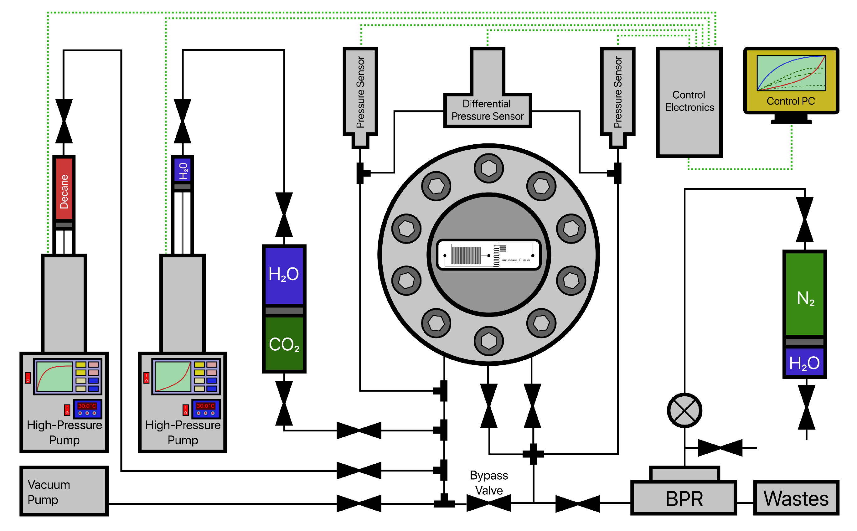
2.1. Microfluidic Assembly

For a microfluidic experiment, a special microfluidic assembly should be used. Conceptually, it consists of the following equipment: a microfluidic chip, a high-pressure and high-temperature microfluidic holder, a high-pressure pump, valves and equipment for visual control.

For the presented research’s goals, a custom-designed and manufactured silicon-glass microfluidic chip was used. For precise fluid control (minimum flow rate was 0.0001 mL/min), two high-pressure and high-temperature laboratory piston pumps (LN-P, Geologika, Novosibirsk, Russia) were used. For the pressure-tight injection of fluid inside the microfluidic chip, a patented microfluidic holder [63] was used; its detailed description can be found in the Supplementary Information (S2). The zero-leakage sealing between the microfluidic holder and microfluidic chip was secured using an oil-resistant hard Buna-N o-ring (1247N132, McMaster-CARR, Robbinsville, NJ, USA). A dual-stage vacuum pump (V-i240SV, VALUE, Wenling China) was used to vacuum all hydraulic system elements. A backpressure regulator (ZF Zero Flow BPR, Equilibar, Fletcher, NC, USA) was used and controlled by gas for outlet pressure control. The injection of CO₂ was performed through the high-pressure transfer vessel. Two high-accuracy pressure transducers (PX01D1-10KGI, Omega, Norwalk, CT, USA) were used for pressure control, and one differential pressure transmitter (PD-39X, KELLER AG, Winterthur, Switzerland) was used to monitor the differential pressure in the system. All these instruments were connected with metal tubes and needle valves. Figure 1 presents the hydraulic system of the microfluidic assembly. One RTD sensor (PR-20-2-100-1/8-2-E-G, Omega, Norwalk, CT, USA) was used to monitor the temperature of the microfluidic holder. Furthermore, six insertion heaters (3618K161, Omega, Norwalk, CT, USA) were used to heat and support the temperature of the microfluidic holder and the chip inside. Then, a special control unit was used to control the system’s electronic components, and a PC station was used for logging during the experiment.

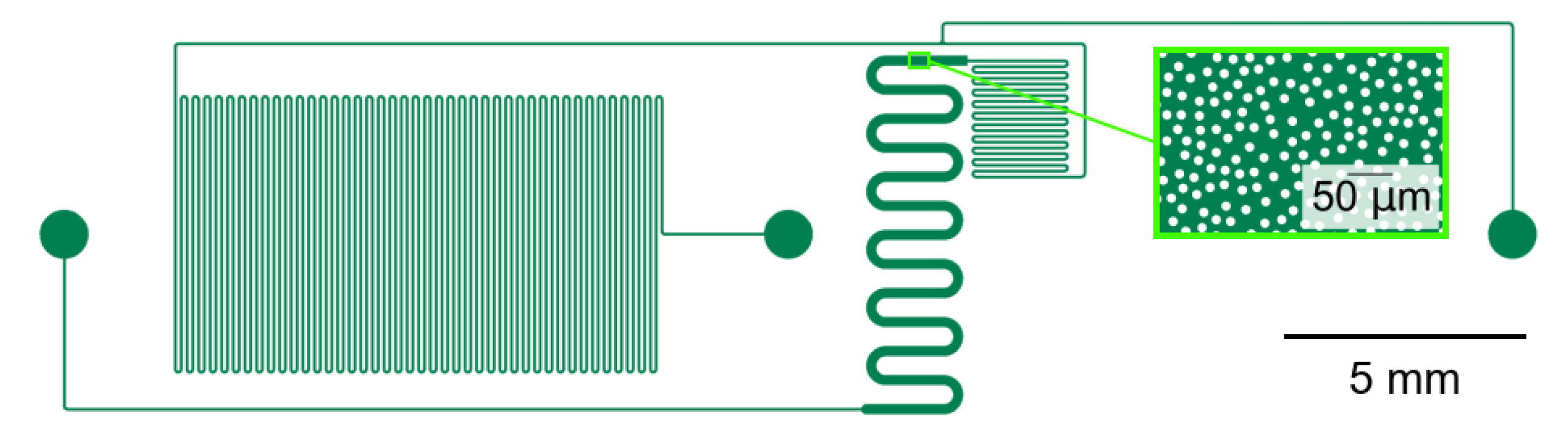
2.2. Microchip Design

The microfluidic chip design was developed specifically for the microfluidic platform described in the previous section. This design had two inlets and one outlet. An additional inlet was used to create a bypass line inside the chip and fill the system at increased fluid flow rates. It helped to bring the injected fluid directly to the porous structure and thereby avoided a significant pressure drop during pumping through the low-permeability zone.

The porous medium of the microchip was represented by a channel 200 microns wide and 20 microns deep with randomly scattered polls (Figure 2). The random structure of non-contiguous cylinders with a diameter of 11 microns was generated using the Python programming language (PoreSpy library [64]: ps.generators.RSA). When the size of the output image and a radius of 5.5 microns were set, the volume fraction parameter was iteratively selected so that the distance between the cylinders was at least 2 microns (one tenth of the etching depth). The final design of the channel had porosity of 74.6% and a volume of 83.26 nl, which was six orders of magnitude less than the standard slim tube.

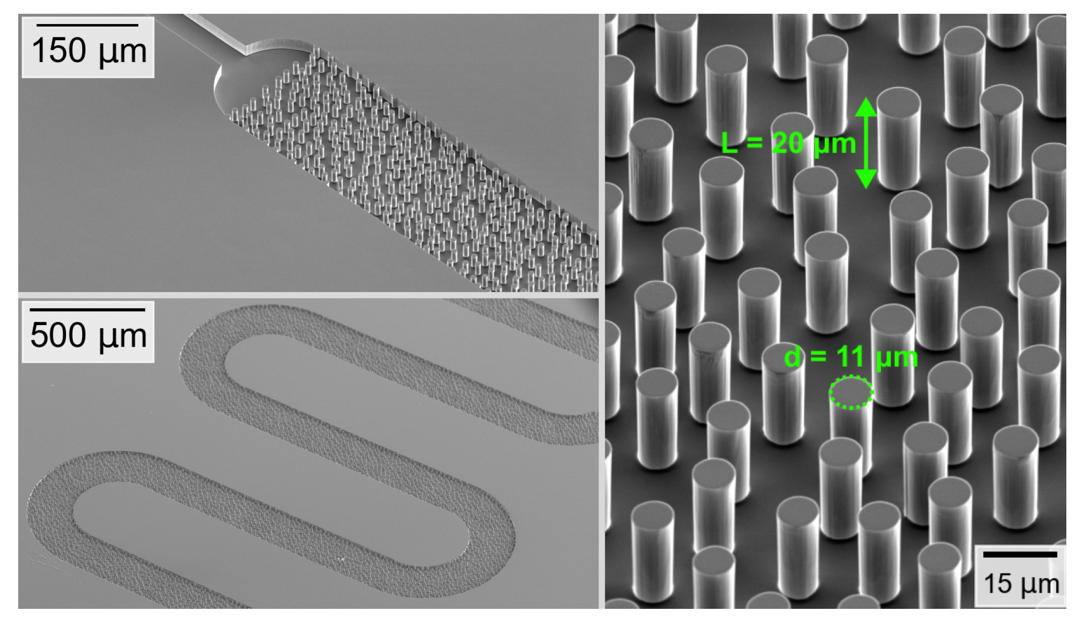
2.3. Manufacturing Process

The creation of microfluidic chips is based on standard technological methods used in the microelectronic industry. A silicon substrate (of any brand and type of conductivity) is chosen as the basis of the microfluidic chip, which is easily subjected to all known technological operations (etching, splicing). The entire technological route can be divided into three main stages: the formation of microchannels, the creation of the fluid inlet/outlet and anode splicing.

In the first stage, the silicon substrate with a diameter of 4 inches was cleaned by the hydrodynamic method. At the next stage, a photoresist (PR) of the AZ4999 brand with a thickness of 2 microns was spin-coated onto the silicon substrate, with a preliminary application of hexamethyldisiloxane (HMDSO) for better adhesion of the photoresist to the substrate. Then, the pattern of microchannels was formed by laser lithography on the Heidenberg DWL2000 installation, followed by photoresist development in 0.96% KOH aqueous solution. The next step in forming the microfluidic chip was the process of deep anisotropic etching of silicon to a given depth by the Bosch method. The critical parameters of the process are the shape of the resulting channels and the roughness of the walls (scallops), which directly depends on the time of the deposition and etching steps. Therefore, a minimum step time was used (less than 1 s) to minimise the walls’ roughness. Inductively coupled plasma (ICP) deposition and etching powers were 1300 W and 1500 W. The etching rate of silicon was 0.3 µm/min, and the photoresist’s selectivity to silicon was 1:87. After the silicon etching process, the residual protective passivation layer and photoresist were removed in oxygen plasma. The photos from the scanning electron microscope of the etched silicon wafer are presented in Figure 3. The next important step in creating a microfluidic chip is the formation of end-to-end fluid input/output channels. Its implementation is possible in several ways: through the etching of silicon by the Bosch method via a rigid mask, mechanical drilling or laser ablation.

When creating the microfluidic chip, in addition to scientific tasks, the problem of the economic feasibility of their manufacturing was solved; the method of laser ablation was chosen as a working method for the formation of through-holes. It is known that the method of laser ablation of a substance is accompanied by a strong effect of surface contamination by removal products. However, we found that the preliminary deposition of a thick layer of AZ4999 photoresist with a thickness of more than 5 microns on the plate surface after the laser ablation process and photoresist removal led to a significant reduction in contamination. According to the economic feasibility assessment, the ratio of the cost of forming through-holes by Bosch etching and laser ablation is ≈100:1, respectively. Hydrodynamic washing of the surface was carried out after forming through-holes in the microfluidic chip. The next stage was the process of anodic bonding of a silicon wafer with borosilicate glass. The main parameters of the anode splicing mode were a substrate temperature of 350 ${}^{\circ }$C, an anode current of 4 mA, an anode voltage of 700 V, a clamping force of 120 N and a splice time of 10 min. The final process in microfluidic chip manufacturing is separating a 4-inch plate into separate chips. The separation process was performed using mechanical cutting on a DISCO DAD circular saw. A photo of the manufactured microfluidic chip and its additional description can be found in the Supplementary Information (S3).

2.4. Fluids and Fluorescent Additive

For the experiments, a combination of standard fluids was used—99% purity n-decane (Sigma Aldrich, St. Louis, MO, USA) and 99.995% purity CO₂ (high-purity carbon dioxide, grade 4.5). To distinguish two phases under a microscope, one of the fluids must be fluorescent. Thus, Nile Red (72485, Sigma-Aldrich, St. Louis, MO, USA), a fluorescent dye soluble in organic solvents and hydrophobic lipids and almost insoluble in water, was added to the n-decane.

For the standard fluids, it is crucial to choose the optimal concentration of additive, since Nile Red’s excitation and emission spectra are highly dependent on the solvent and vary widely in both shape and intensity [65]. For n-decane, the volumetric mixing ratio of 1:100,000 was chosen, which appeared to be optimal [4,66]. C₁₀H₂₂ containing Nile red in higher concentrations was found to leave a vast amount of additive in the matrix, affecting the flow structure.

3. Methods

3.1. Experimental Procedure

The experiment begins with the assembly of a microfluidic platform. Next, the selected chip is installed on the lower part of the microfluidic holder with sealing o-rings, pressed with a specially manufactured sapphire crystal and the upper part of the microfluidic holder, which should be tightly bolted to withstand high pressure during the experiment. Next is the preparation of the fluids. N-decane is mixed with a fluorescent additive at a given concentration and fills the pump head; carbon dioxide is fed into a piston vessel, from which it will subsequently be injected by pumping water at a given flow rate.

Afterwards, the microfluidic platform is connected to a pre-prepared system of hydraulic lines, thoroughly cleaned and dried after previous experiments. Special piston heaters are inserted into the platform and switched on to maintain the set temperature with an error of ±0.2 ${}^{\circ }$C. Then, the system is vacuumed for 30 min. After the successful connection of the pump line to the hydraulic system, C₁₀H₂₂ injection starts with a constant flow rate through the bypass. The bypass is closed as soon as the n-decane begins to exit on the backpressure regulator (BPR), and the filling continues to other parts of the system. When the system is fully saturated, up to one hundred pore volumes of n-decane are pumped through the microfluidic chip to remove possible residues left after the manufacturing stage. Further, the pressure on the BPR rises stepwise to the test pressure.

Many microfluidic tests rely on the precise regulation of the surface wettability for successful functioning. The MMP provided here does not depend on the wettability of the surface, but rather on the physicochemical parameters of the fluids, the pressure and the temperature [6,67]. If the experiment is conducted for the first time, then single-phase filtration through the microchip is carried out at a constant flow rate. It allows the calculation of the permeability of the designed porous structure. After a sufficient time, the n-decane injection is stopped, and the inlet valve is closed.

CO₂ injection starts through the bypass of the microchip, displacing C₁₀H₂₂ at a high flow rate from all inlet lines and creating an interface between the two fluids at the T-junction before the pore structure. When the n-decane stops exiting on the backpressure regulator, the outlet valve is opened and gas injection starts to the porous structure, maintaining differential pressure of no more than 0.01 MPa. The filtration video is recorded on a digital microscope for subsequent video processing to obtain a change in the displacement coefficient over time.

Traditional slim-tube tests are required to control the flow rates and pumped pore volumes to determine the MMP value. The sweep coefficient is determined at the exact value of the pumped pore volume, where all parameters cannot be changed from test to test. In our case, the visual method is used to determine the interaction of gas with liquid. Thus, to control the consistency of the experimental duration, the period from the gas entry to the porous structure to five seconds after the gas breakthrough is taken.

In the next experiment, the system is washed with solvents, purged and dried to exclude the existence of residual fluids for the following experiments.

3.2. Numerical Modelling

A 2D Computational Fluid Dynamics (CFD) simulation of the experimental work is carried out. The primary purpose of the numerical simulation is to reproduce the experimental results and test the possibility of obtaining future predictions of the MMP of CO₂–C₁₀H₂₂ systems at different temperature values outside the scope of the experimental work.

3.2.1. Governing Equations

The governing equations for the numerical model are grouped into two parts: the equations that describe the immiscible/near miscible flow and the set of equations that describe the miscible flows.

Immiscible Flow

The immiscible flow is governed by a coupling between the Navier–Stokes equation and an interface tracking method. The Navier–stokes equation is described by solving the continuity equation (Equation (1)) and the laws of conservation of momentum (Equation (2)). These sets of equations assume that the simulated fluid is Newtonian and incompressible. At the pore scale, the viscous forces dominate the inertia forces. Hence, the inertia term in the Navier–Stokes equation is dropped, and the flow is regarded as a creeping flow. The effect of gravity on the flow is neglected, while the source term (${\mathrm{F}}_{\mathrm{st}}$) is introduced into the Stokes equation by the interface tracking method (phase-field method).

$$\nabla ·\overrightarrow{u}=0$$

(1)

$$\rho \left(\frac{\partial \mathrm{v}}{\partial t}+\left(\mathrm{v}·\nabla \right)\mathrm{v}\right)=-\nabla \mathrm{p}+\rho g+\mu \left(\nabla \mathrm{v}+{\nabla }^T\mathrm{v}\right)+{\mathrm{F}}_{\mathrm{st}}$$

(2)

The phase-field method implements a boundary condition to express the effect of the wettability between the solid surface and the fluids. In this work, the wettability of the walls was regarded as a constant (26${}^{\circ }$), and the effects of changing wettability and hysteresis were negligible. In addition, the capillary forces were higher; hence, the impact of diffusion was neglected.

Miscible Flow

The miscible displacement was modelled by coupled physics between the Navier–Stokes equation (Equation (2)) and the convection–diffusion equation (Equation (3)).

$$\frac{\partial c}{\partial d}=\nabla ·\left(D\nabla c\right)-\nabla ·\left(\mathrm{v}c\right)+R$$

(3)

where c—concentration, mol/m${}^3$; D—diffusivity coefficient, m${}^2$/s; v—velocity, m/s; R—source term of the concentration of a species, mol/m${}^3$. Under the miscible conditions, the interfacial force between the two fluids approaches zero; hence, it disappears. The fluid–fluid interface is controlled by the rate at which the injected fluid diffuses into the displaced fluid. Therefore, the mixing of the fluids changes the rheology (density and viscosity) of the resultant fluid mixture. Furthermore, the consequent mixed fluid swells and increases in mobility compared to the original displaced fluid. However, in this work, the set of equations used assumes the incompressibility of the two fluids and the resultant mixture. Hence, the effect of fluid swelling is neglected. In contrast, the potential changes in the chemical composition of the resultant fluid mixture are described by the continuous averaging of the fluid mixture in the domain at every computational time step. The resultant fluid density and viscosity are calculated by Equations (4) and (5), respectively [68].

$$\rho \left(c\right)=\frac{c-c_0}{c_{inj}-c_0}{\rho }_{C{O}_2}+\left(1-\frac{c-c_0}{c_{inj}-c_0}\right){\rho }_{oil}$$

(4)

$$\mu \left(c\right)={\left[\frac{c-c_0}{c_{inj}-c_o}{\mu }_{c{0}_2}^{-0.25}+\left(1-\frac{c-c_0}{c_{inj}-c_0}{\mu }_{oil}^{-0.25}\right)\right]}^{-4}$$

(5)

where $c_0$—initial concentration of the fluid in the domain, mol/m${}^3$; $c_{inj}$—concentration of the injected fluid, mol/m${}^3$; $\rho \left(c\right)$, $\mu$—density, kg/m${}^3$ and viscosity, Pa·s at each time step. The mole fraction of the the two fluids in the simulated domain is computed by the average concentration of CO₂ and n-decane in the domain.

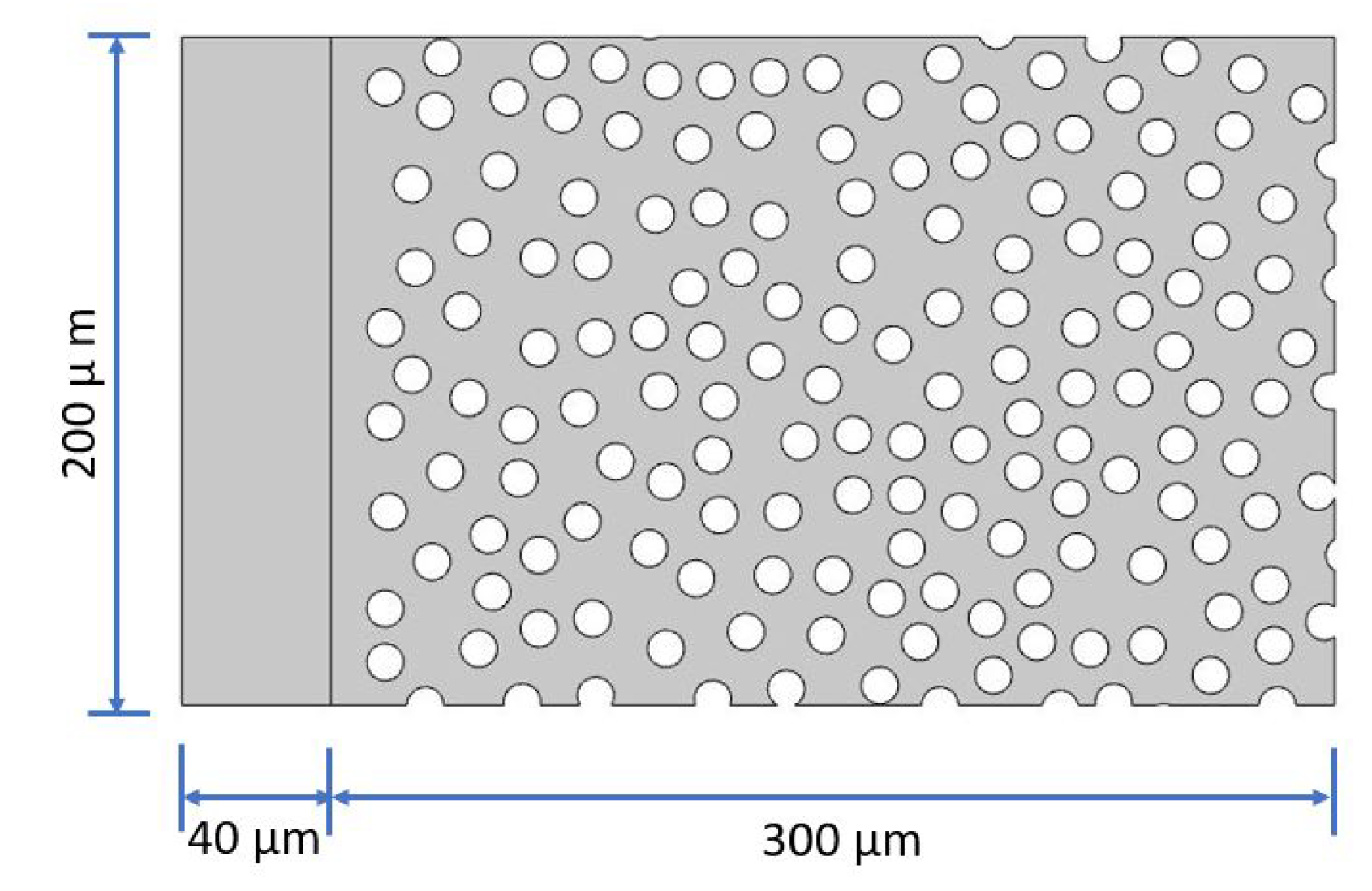
3.2.2. Computational Domain and Boundary Conditions

Simulating the entire volume of the microfluidic chip used in the experimental work required high computational power. Therefore, to overcome the problem with computational costs, a section of the model was generated to mimic the entire experimental model. The simulated volume (SV) is presented in Figure 4. The SV is 200 µm wide and 300 µm long, with an extended inlet of 200 µm × 40 µm to establish a fully developed flow at the inlet. The surface area of the SV is $4.68\times {10}^{-8}$ m${}^2$/s, while the surface area of the entire model used in the experiment is $4.3503\times {10}^{-6}$ m${}^2$/s. The computed porosity of the SV is 78%, which is approximately 5% more than the porosity of the entire model (74%).

At the initial time, the SV was 100% saturated with n-decane, while the extended inlet was 100% saturated with CO₂. This aimed to ensure a fully formed flow boundary condition at the inlet of the channel; a fully formed flow inlet velocity ($v_o$) boundary condition for CO₂ was specified. At the outlet of the SV, the pressure boundary condition was specified to be 0 MPa. The differential pressure across the channel was determined by the inlet velocity of CO₂ ($v_0$). The value was less than 0.01 MPa, as regulated in the experiment. A no-slip boundary condition was applied on the impermeable walls of the channel.

Table 1. Input parameters of numerical model.

Parameter	Unit	Value
Pressure (p)	MPa	6.0	6.25	6.5	6.75	7.0
Density (C10H22)	kg/m${}^3$	727.42	727.62	727.81	728.81	728.39
Density (CO2)	kg/m${}^3$	171.44	187.37	206.44	230.77	266.56
Viscosity (C10H22)	mPa.s	846.67	849.14	851.54	853.98	856.43
Viscosity (CO2)	mPa.s	17.76	18.21	18.777	19.576	20.91
Contact angle ($\theta$) a	${}^{\circ }$	26	26	26	26	-
IFT (F) a	N/m	0.003	0.002	0.00105	0.0001	-
Diff. coeff. ($D_0$) b	m${}^2$/s	-	-	-	-	$1.24\times {10}^{-9}$
Temperature (T)	K	303.15
Inlet velocity (u)	m/s	$3.0984\times {10}^{-5}$

^a Immiscible displacement; ^b miscible displacement.

shows the input parameters for the various simulations. The viscosity and density of the pure fluids under the given pressure and temperature conditions were obtained from [69] and the values of IFT were taken from [70]. The contact angle between decane and CO₂ was obtained from the results of the experiment presented by [71].

4. Results

4.1. Experimental Section

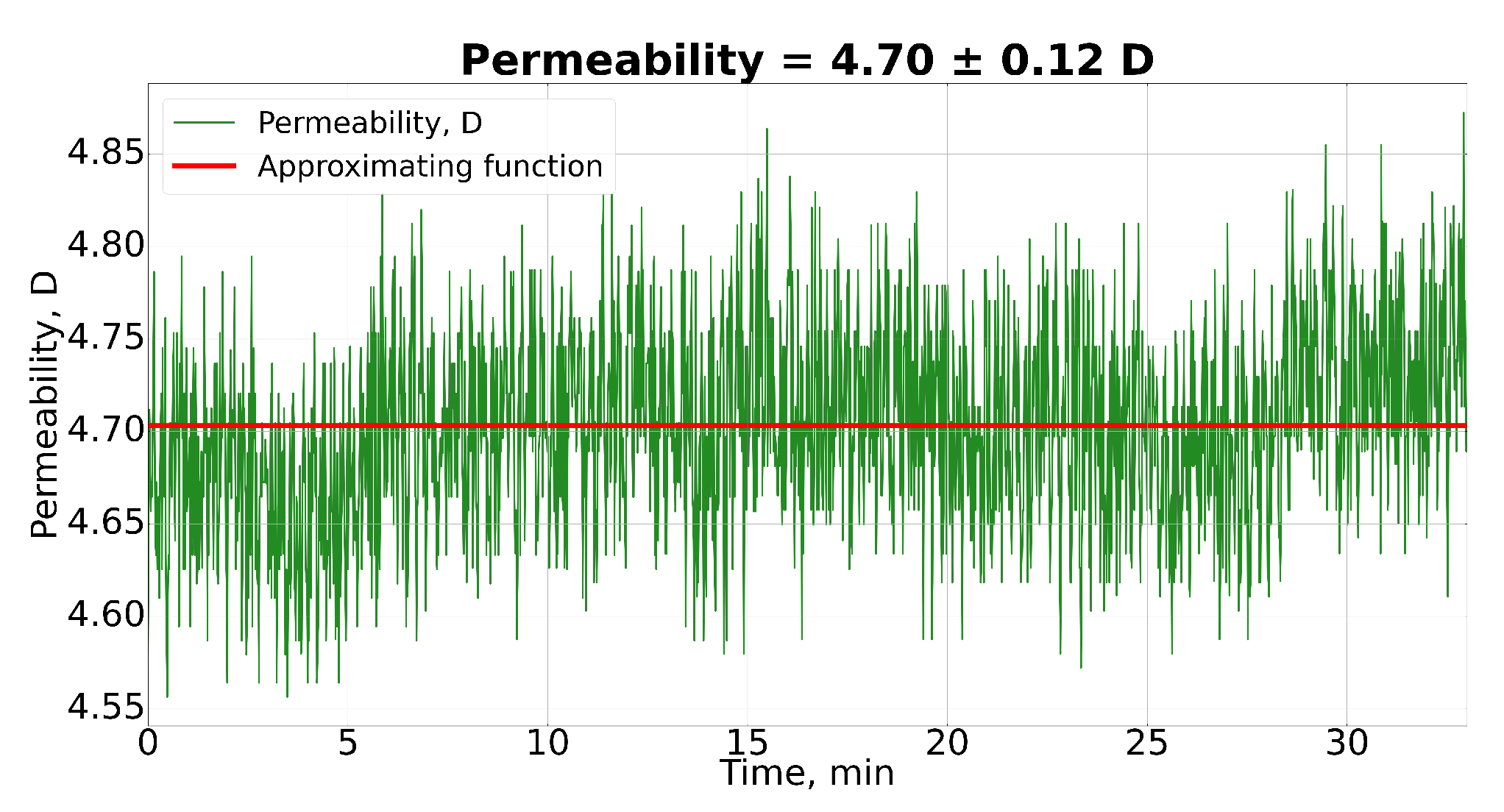
4.1.1. Permeability Determination

The experimental part began with the single-phase filtration of n-decane through a porous structure. The injection was performed with a constant flow rate (0.025 mL/min), and changes in differential pressure were recorded. Thus, the value of permeability was calculated using the Darcy equation:

$$k=\frac{q·\mu ·l}{A·P_{dif}}$$

(6)

where q—flow rate, ml/min; $\mu$—dynamic viscosity, Pa·s; l—length of the porous structure, µm; A—cross-section of the porous structure, µm²; $P_{dif}$—differential pressure, MPa. Figure 5 shows the calculated permeability over time due to the changing differential pressure. The approximating function was plotted to obtain a single permeability value. The uncertainty of permeability was obtained by considering the accuracy and precision of the pressure sensors, pump and thermocouple (S1). The definition of permeability was substantial for preliminary pressure drop estimation and further use in simulators.

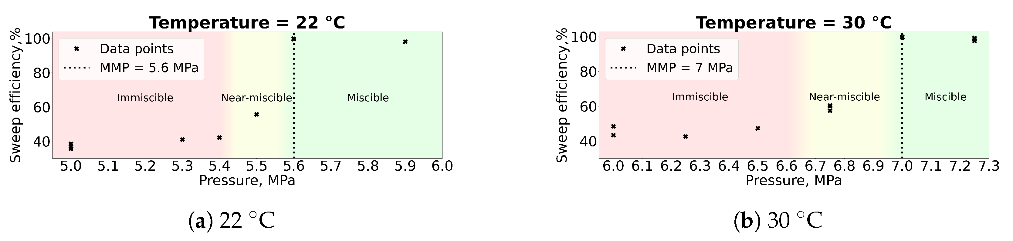
4.1.2. MMP Determination

Raw Data

A series of tests were carried out to determine the minimum miscibility pressure of C₁₀H₂₂ and CO₂ for room temperature (22 ${}^{\circ }$C) and 30 ${}^{\circ }$C. The starting pressure of each experiment was chosen based on a literature review and was far less than the MMP value to achieve immiscible displacement.

Into the fully saturated channel with n-decane, CO₂ was injected, which propagated through a porous medium with a visual interface (Figure 6b). The fingering effect led to partial n-decane displacement during such gas breakthrough.

For the subsequent experiments, the system was cleaned and again saturated with fluorescent n-decane. Subsequently, the pressure at the backpressure regulator was increased, and the next experiment started. Experiments continued until the injected gas propagated without gas fingering but with a stable front (Figure 6c). Miscible CO₂ entirely displaced n-decane and left no residual oil.

Qualitatively, it was observed that there was a difference in how the front proceeded for the immiscible and miscible cases, which helped to define the MMP values (5.6 MPa for room temperature, 7 MPa for 30 ${}^{\circ }$C). Further, these values needed to be validated quantitatively after video processing.

Video Processing

A particular function was written in the Python programming language that allowed the processing of the video data for each series of experiments (selected temperature). As input, the code was given a set of videos. The first and last frames were cut from every video, which helped to configure the algorithm.

Further, the images were cropped so that only a porous channel remained inside the frame. For these frames, the brightness was increased by superimposing a Gaussian blurred image on an original frame (OpenCV library: cv2.blur, cv2.addWeighted).

The next step was colour filtering. For all the frames taken from the video, a particular (same for all videos) colour mask was found to leave only the desired colour, removing possible uncertainties of illumination from the microscope. It was crucial to validate the resulting mask to achieve the proper processing of frames. The channel with fluorescent n-decane should ultimately retain its shape and colour saturation for the first few frames. The final frames should either show the complete vanishing of colour (miscible displacement) or incomplete disappearance (immiscible displacement), but with the preservation of the gas flow structure (OpenCV library: cv2.inRange, cv2.bitwise_and).

The final stage in configuring the algorithm was the binarisation of frames using the adaptive thresholding function (OpenCV library: cv2.adaptiveThresholding). By selecting the values of the configurable parameters, the size of the neighbourhood area and a constant for subtraction from the mean sum of the neighbourhood pixels, binary frames were obtained, where white represented n-decane and black represented CO₂ or the zone not participating in the experiment.

Finally, the algorithm setting produced four frames for each video: two original and two processed frames. Figure 6 shows an example of such processing for miscible and immiscible flows. If the algorithm setting is successful, it can be applied to all videos.

4.1.3. Final Results

After successful video processing, we obtained binarised frames as output, for which the displacement coefficient was recalculated at each time step and plotted with the frame. The sweep efficiency coefficient (K) was calculated as follows:

$$K=\left(1-\frac{N_{whiteend}}{N_{whitestart}}\right)·100\%$$

(7)

where $N_{whitestart},N_{whiteend}$—number of white pixels before and after the experiment.

The function was also used to plot graphs of the changing sweep efficiency versus time for each video based on these frames. Examples of the graphs for the immiscible and miscible cases are shown in Figure 7. As can be seen, each experiment was conducted precisely as in the described procedure. The experimental videos were taken from the moment that the gas reached the porous structure to five seconds after the gas front reached the outlet. Additionally, binarised frames were combined for each experiment to create the processed videos (Movies S1 and S2).

Finally, the algorithm combines the final values of the sweep efficiency for each temperature and plots them in graphs (Figure 8). The point at which the displacement coefficient reaches a value close to 100% for the first time is taken as the minimum miscibility pressure value. The quantitative analysis of changes in sweep efficiency for each video gives additional confirmation of the pressure when miscibility occurs. Therefore, for 22 and 30 ${}^{\circ }$C, we obtain the MMP values of 5.6 and 7 MPa, respectively, which a literature review can further validate.

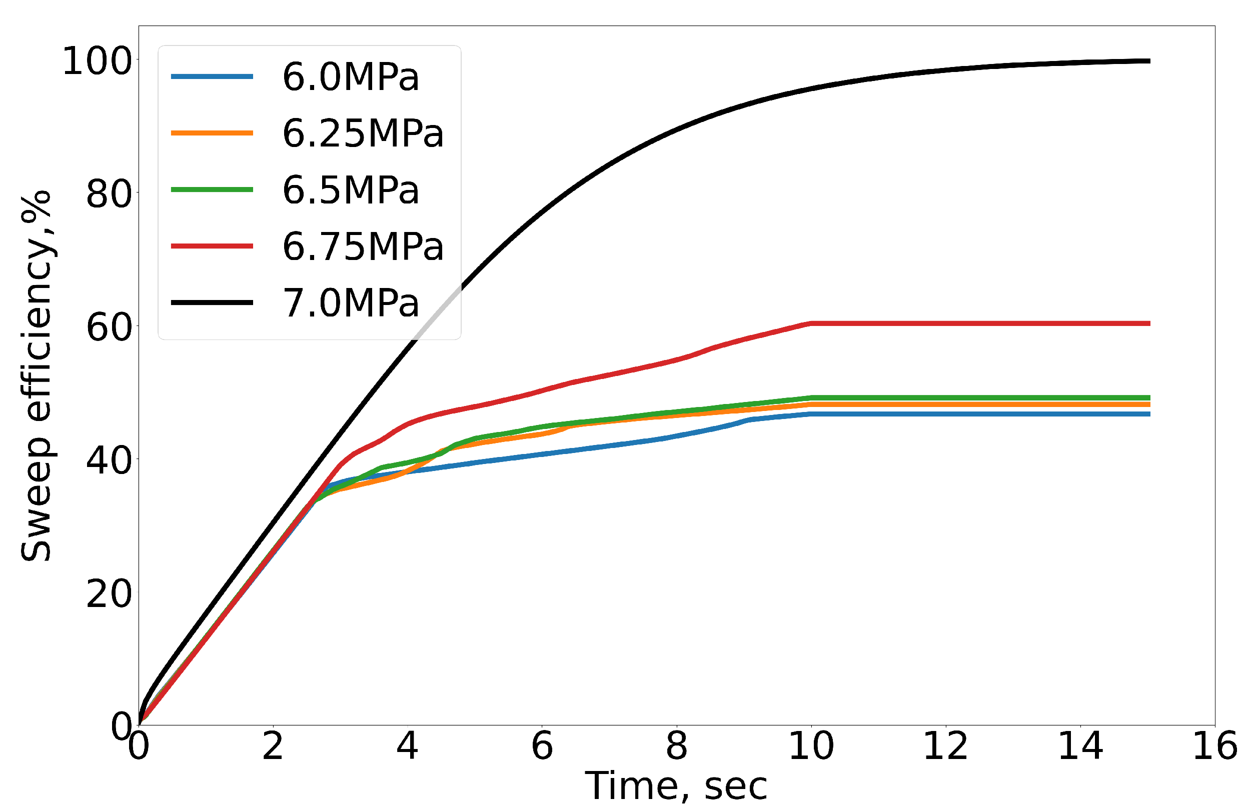
4.2. Results of Numerical Simulation

To ensure accurate results from the numerical model, the mesh quality was examined to determine the most appropriate mesh for modelling. The number of mesh elements was increased until the result of the simulation remained fairly constant for the simulated models.

The RMSE between the coarse and fine mesh was 2.319, while the RMSE between the normal and fine mesh was 0.291. The computation cost for the simulation increased by 1.14% when the number of mesh elements was increased by approximately 5%. Similarly, the computational cost increased by 4.9% when the number of mesh elements was increased by 12%. The statistics of the generated meshes are presented in

Table 2. Mesh statistics.

Mesh Type	No of Elem.	Min Elem. Quality	Avg Elem. Quality
Fine Mesh	127845	0.02681	0.78
Normal Mesh	53697	0.07488	0.78
Coarse Mesh	10494	0.03859	0.69

and the Supplementary Information (Figure S4). The value of the RMSE indicated that there was no significant difference between the sweep efficiency of the normal and the fine meshes. Moreover, the higher the number of meshing elements, the higher the computational cost. Hence, the normal mesh was used for further simulations to reduce the computational cost.

The results from the microfluidic experiment gave insights into the set of equations to implement for the experimental pressure and temperature ranges. Furthermore, for temperature and pressure ranges with indications of near-miscible flow, the same set of equations was used (Equations (1) and (2)). As the fluid approaches miscibility, the interfacial force decreases and the clear interface between the two fluids reduces. This concept was implemented in the numerical model by decreasing the value of IFT for the given fluids for the simulation of the near-miscible region. The interfacial force between the two fluids was adjusted based on the reported literature. In contrast, for the miscible displacement, the value of IFT approaches the minimum and, hence, no clear interface between the two fluids exists; rather, a thick zone of mixing of CO₂ and n-decane could be seen [72]. In this simulation, the IFT between the two fluids under the miscible conditions was neglected. Simulations of immiscible, near-miscible and miscible flows were performed at 30 ${}^{\circ }$C. Overall, five pressure points were computed, 6.0 MPa, 6.25 MPa, 6.5 MPa, 6.75 MPa and 7.0 MPa, as shown in Figure 9. The sweep coefficients of the various simulations were computed by the fluid volume fraction at every time step. From the simulated models, the simulation at 7 MPa attained a 100% sweep coefficient, while the sweep coefficients of the simulations at 6.75 MPa, 6.5 MPa, 6.25 MPa and 6.0 MPa were 60.35%, 49.17%, 48.18% and 46.74%, respectively, as shown in Figure 9. A video representation of the simulated models is included in the Supplementary Information (Movies S3–S7).

5. Discussion

Two series of tests were carried out on the model fluids (CO₂– C₁₀H₂₂), allowing us to identify various approaches that help to determine the MMP value. For instance, the gas front propagation changes when the two-phase filtration transforms from immiscible to miscible. Thus, even without processing the experimental video, we may derive the value of the minimum miscibility pressure by determining the pressure value throughout the experiment. However, subsequent binarisation is needed to confirm the obtained MMP values by calculating the sweep efficiency coefficient for each experiment.

In order to validate our results, it was necessary to conduct a literature review analysing the experiments on MMP with the chosen gas–liquid system under particular conditions. All of the literature sources found are shown in

Table 3. MMP of CO₂ in C₁₀H₂₂ using different techniques.

T-re, ${}^{\circ }$C	MMP, MPa	Method	Source
20	5.4	Microfluidics	Bao et al. [73]
20	5.5	X-ray CT	Liu et al. [74]
20	5.6	MRI a	Song et al. [75]
22	5.6	Microfluidics	this article
30	6.4	Microfluidics	Bao et al. [73]
30	6.7	X-ray CT	Liu et al. [74]
30	6.7	MRI	Song et al. [75]
30	7	Microfluidics	this article
37.8	7.7	X-ray CT	Liu et al. [74]
37.8	7.8	MRI	Song et al. [75]
37.8	8.0	VIT	Ayirala and Rao [76]
37.8	8.3	Slim-tube (0.95) b	Elsharkawy et al. [77]
37.8	8.6	Slim-tube (BOP) c	Elsharkawy et al. [77]
37.8	8.8	RBA	Elsharkawy et al. [77]

^a Magnetic resonance imaging; ^b pressure at 95% oil recovery; ^c pressure at breakover point.

.

Nine experiments were performed for the first set of tests at 22 ${}^{\circ }$C (room temperature), obtaining the value of 5.6 MPa. The closest values of the minimum miscibility pressure for n-decane and CO₂ were found for temperature 20 ${}^{\circ }$C, where the MMP value was measured by X-ray CT, nuclear magnetic resonance and the microfluidic approach. It can be noticed that the difference between the microfluidic test of [73] and the conducted test is 0.2 MPa, which is explained by a slight temperature difference. Nevertheless, compared to other tests, the pressure values practically do not differ, which may indicate the inaccuracy of a particular experiment. Since the test at a temperature of 22 ${}^{\circ }$C was a trial, and the temperature data differ from those published in the literature sources, it was decided to validate the accuracy of the measurements on another test conducted under a controlled temperature at 30 ${}^{\circ }$C.

For 30 ${}^{\circ }$C, thirteen tests were carried out to define a minimum miscibility pressure equal to 7 MPa. Comparing this value with the data published in the same articles shows that the difference is significant. A possible reason for the relative difference of 8.6% between the microfluidic experiment and the one presented in our article may be the microfluidic chip design differences and the experimental procedure.

For their experiments, Bao et al. [73] used a microchip with two straight microchannels (100 µm wide) and two dead-end channels with a width of 5 µm, branching off from the main channel. This width of the dead-end channel was selected to avoid channel collapse during manufacturing and to allow the visualisation of fluid phases with an optical microscope. The MMP value was determined based on the relative change in intensity. Therefore, incorrect calibration by intensity or false detection in such a small channel could have caused the significant difference in the MMP value compared to our microfluidic experiment.

The relative difference of 4.3% arising from computer tomography and magnetic resonance data is explained as follows. Suppose that we re-examine Table 3; at a temperature of 37.8 ${}^{\circ }$C, the standard slim-tube tests show a value greater than the ones considered at a temperature of 30 ${}^{\circ }$C. Therefore, it can be assumed that these tests slightly underestimate the actual values of MMP, being the reason for the difference from the X-ray and MRI techniques. Moreover, for these experimental methodologies, as in the microfluidic test on dead-end channels, the MMP value was determined based on the relative change in intensity. In our microfluidic experiment, it was not possible to obtain such a difficult-to-determine parameter as the intensity while at the same time allowing us to qualitatively and quantitatively assess whether the fluids were mixed during two-phase filtration or not. As a result, it is reasonable to conclude that the microfluidic test described in this article is most closely related to the slim-tube test, which is the widely accepted petroleum industry standard.

This is confirmed by the fact that the microfluidic model meets the same requirements that are imposed on minimum miscibility studies using the slim-tube (ST) test [51,78]:

• The length of the microfluidic ST is rather long to provide the necessary zone for immiscible displacement while not obscuring the overall impact of miscible displacement.
• The width of the microfluidic channel is modest, which reduces the influence of gravity and fingering effects.
• The injection rate is controlled to be constant and relatively low, but remains unimportant since the system is sufficiently lengthy.

Although the ST test is recognised as a standard, there are still no standard criteria for MMP determination in the petroleum industry. Some researchers, for instance, take the moment at which specific oil recovery occurs after a particular pore volume is injected [79] or at a certain gas–oil ratio [80]. Amao et al. [81] tried to exclude difficult-to-determine pore volumes injected by introducing other cut-off parameters (instantaneous recovery rate and oil recovery rate), which appeared to be sufficiently reliable. As can be seen, there is still no standard procedure, and this is unfeasible since the size of the tubes and their filling vary in different laboratories. Thus, for experiments on the microfluidic ST analogue, it was necessary to set new, unique criteria by which the end of a particular run could be determined. For this type of microfluidic test, it was suggested to take the moment of five seconds after the gas breakthrough through the porous medium. Foremost, unlike the standard test on a slim tube, where the moment of gas breakthrough is determined based on various indirect and complex parameters described above, this type of experiment allows us to see the front passage visually. Thus, it allows the tracking of the filtration time through the microfluidic channel with accuracy of a fraction of a second. Secondly, an additional interval of five seconds was maintained for each experimental point, which helped us to prove that the sweep efficiency coefficient had reached its maximum after gas front breakthrough under these particular thermobaric conditions.

After we had determined how to perform and process a specific experimental point, it was necessary to choose a method for the final data interpretation. Due to the long duration of the ST experiment, as well as its high cost, a few experimental points are often obtained. All of them are plotted on the graph of the sweep efficiency coefficient’s dependence on pressure, where the minimum miscibility pressure is determined by a break in slope [51]. Such a break is often determined by constructing two approximating straight lines, the intersection of which splits the graph into two zones of miscible and immiscible displacement. Therefore, even a small inaccuracy in the construction of such approximation lines can significantly affect the final MMP value.

Previous studies have demonstrated that surface wettability is one of the main parameters that affects the sweep efficiency in immiscible multiphase flow systems [82,83,84]. The work by Li and Fan [71] demonstrated that for a CO₂– C₁₀H₂₂ system, the contact angle between the two immiscible fluids does not change, regardless of the temperature, the pressure or the surface material (hydrophilic or hydrophobic). Based on this understanding, the contact angle was assumed constant (26${}^{\circ }$) in the presented research. Thus, the values of the sweep efficiency coefficient and the MMP values were not influenced by the wettability.

One of the main advantages of microfluidic experiments is the ability to conduct a large number of tests in a short period of time, which significantly simplifies the approach to interpreting the results. Similarly to the standard ST test, all the points of the experiments, without exception, were displayed on the final graphs (Figure 8). For each temperature on the final graphs, three zones were allocated, corresponding to immiscible, near-miscible and miscible regimes. The immiscible displacement zone was coloured with red and characterised by a slight fluctuation in the displacement coefficient but, at the same time, a constant, relatively low value from 35 to 45% at 22 ${}^{\circ }$C and from 40 to 50% at 30 ${}^{\circ }$C. The following (yellow) zone of the near-miscible regime was characterised by a slight increase in the displacement coefficient while not reaching values close to 100%. Finally, the zone of complete miscibility is highlighted in green and displays the zone where the gas was thoroughly mixed with the liquid while achieving a displacement coefficient close to 100%.

The relative error in the sweep efficiency of the numerical simulation and experimental results was evaluated. The results of the numerical simulation were in good agreement with the experimental results. The error between the numerical simulation results and the experiment was within the range of 0.25–17%. The lowest error (0.25%) was recorded for the miscible displacement (7 MPa), whilst the highest error (17%) was recorded for the immiscible case at a pressure of 6.25 MPa.

The curve of the sweep coefficient can be divided into three main stages. The first stage for the immiscible displacement occurred between the initial time step and lasted approximately three seconds—a sharp linear increase in the sweep coefficient was recorded at this stage. Next, the injected CO₂ moved along the higher-permeability zone, displacing all the n-decane along its path (Figure S6). The second stage of the simulation included the moment that the injected CO₂ reached the outlet of the channel. Prior to this stage, a preferable path of CO₂–C₁₀H₂₂ displacement was created; hence, the successive filtration of CO₂ occurred mainly along this path (breakthrough zone) due to low flow resistance as compared to the first stage. Nevertheless, slight displacement was observed in other sections of the domain, which increased the sweep efficiency. The final and later stage is characterised by CO₂ flow through only the established channels and no significant increase in the sweep coefficient, as shown in the Supplementary Information (Figure S6). The results of the miscible displacement showed similar stages of the displacement and mixing of the two fluids. However, these stages are due to continuous changes in the average change in the rheology of the fluid–fluid mixture in the entire simulated domain.

At higher pressure, the IFT between the two fluids is lower. Hence, the flow is easily redirected towards the dominant flow path. The patches are located between two pores with a narrow opening in the transverse direction to the flow rate. The visual representation of the flow velocity shows that the preferred flow path had a higher velocity gradient than the other sections of the porous medium for the immiscible flow displacement. Numerical modelling shows a higher velocity distribution in the preferred flow path for both the miscible and immiscible flows (Figure S5).

The velocity distribution explains the heterogeneity associated with unconventional reserves. The higher-permeability zones dominated the fluid displacement and resulted in severe fingering of the injected fluid under immiscible conditions. The higher the IFT between the two liquids, the higher the magnitude of fingering. In contrast, the impact of domain heterogeneity does not result in fingering under the miscible condition. In this work, while a plug-like flow was established, the diffusion of the injected solvent (CO₂) was also observed. The density and viscosity of the binary mixture formed by the mixing of CO₂ with n-decane were computed at every time step by Equations (4) and (5), respectively. Figure 10 presents the resultant average density and viscosity over the simulated porous domain. The convection and diffusion transport work simultaneously in the case of miscible flow. While the injected volume of CO₂ increases, the importance of n-decane decreases through the combination of the mixing of the two fluids at the fluid–fluid interface and the exiting of pure n-decane from the simulated domain. The mixing of the fluids at the fluid–fluid interface is controlled by diffusion and convection. The results show that both the density and the viscosity decrease as the injected pore volume of CO₂ and the binary mixture increases in the simulated domain. The Peclet number (Pe = $uL/D$) was computed to estimate the dominant mechanism for the simulated porous medium, where u is the average velocity of the flow, L is the channel’s characteristic length and D is the diffusion coefficient. The value of the Peclet number is 7.35. The result indicates that the simulated model’s convection transport is dominant over diffusive transport.

Generally, the presented approach was introduced to replace conventional experiments: the rising bubble apparatus and the slim-tube test. The RBA approach for the measurement of MMP values is qualitative and relies on visual observations to determine miscibility. Therefore, this method has some subjectivity and lacks quantitative information, resulting in arbitrariness in miscibility determination. Moreover, this test is not suitable for complex compositions, where miscibility occurs not in condensing or vaporising but in a combined mode. However, this test is relatively fast, cheap and requires smaller fluid quantities compared to slim-tube techniques. The slim-tube experiment is known as the standard in measuring MMP values, but, at the same time, there are no standard criteria for the methodology or the slim tube itself. Furthermore, the slim-tube test is a time- and volume-consuming approach. While each displacement run under specified pressure takes around two days, cleaning and re-saturating operations lead to a time cost of at least a week for the determination of one pressure point for an oil–solvent system. The microfluidic approach presented in this article eliminates most of the drawbacks of traditional tests. Such tests are more accurate and reliable than both the slim-tube test and the rising bubble apparatus for complex oil systems. Each run of the experiment under certain thermobaric conditions helps to differentiate miscible from immiscible injection, both at the qualitative and quantitative levels. However, microfluidic tests require specialised expertise and equipment.

The experiments were conducted on pure fluids that mix at first contact, unlike real reservoir oil. However, it is expected that such microchip geometry will allow the multi-contact miscibility of crude oils to be obtained by creating relative motion between the two fluids during filtration through the porous channel. Furthermore, the presented microfluidic technology allows the repetition of MMP measurements at different temperatures and pressures for the same geometry. This was proven by conducting several experiments for the same pressure value under a constant temperature. Thus, the technical challenges that usually relate to experiments with traditional tests can be eliminated.

6. Limitations and Future Studies

Despite significant improvements in the required time and fluid volumes for MMP determination, it is essential to highlight current microfluidic technology’s technological challenges and limitations.

• The significant reduction in the porous medium’s volume inside the microfluidic chip necessitates precise fluid control, either by flow rate or differential pressure. The microfluidic experiment does not withstand the effects of pulsatile flow.
• Currently, it is not possible to control the composition of the fluid in situ in the microfluidic chip. Moreover, the volumes of the fluids are too small to be analysed by conventional gas chromatographic methods.
• The quality of images obtained from the microfluidic experiment requires a trade-off between magnification and field of view. Our microfluidic model allowed us to visualise the immiscible and miscible fluid flows along with the whole distance of the main tortuous channel.
• The error between the numerically simulated results and the experimental results could be minimised by increasing the dimensions of the simulated volume of the model in future studies, if there is a trade-off between the simulated volume and the computational cost due to an improvement in computational power.
• The presented microfluidic chip geometry allowed us to observe the miscibility zone of C₁₀H₂₂ and CO₂ inside the microfluidic channel, but experiments with real fluids using this geometry are required.
• It is necessary to develop a strict experimental procedure in further studies to address the above technological challenges.

7. Conclusions

The minimum miscibility pressure of n-decane and CO₂ was investigated by microfluidic laboratory experiments. Numerical simulations were conducted to verify the accuracy of the CDF simulation of a section of the domain. Conclusions based on the results are as follows.

• For pure C₁₀H₂₂ and CO₂ at temperatures of 22 and 30 ${}^{\circ }$C, the MMP values of 5.6 and 7 MPa were obtained, respectively.
• The MMP values determined using microfluidic technology are in good agreement with MMP measurements obtained by other methods described in the literature. For instance, the relative difference for 30 ${}^{\circ }$C is between 4 and 9%.
• The conducted experiments allowed us to define a mechanism to determine the minimum miscibility pressure, both quantitatively and qualitatively.
• The presented microfluidic technique with a special microfluidic chip with a heterogeneous porous medium, compared to the traditional slim-tube test, required a much smaller fluid volume (1 mL, approx.) and exceeded the maximum of one hour for the preparation and experiment itself.
• The simulation of a section of the entire domain (SV) yielded results in good agreement with the experimental results.
• The sweep efficiency of CO₂ increases with increasing confining pressure due to the decreasing IFT between C₁₀H₂₂ and CO₂ under the immiscible condition.
• Numerical modelling showed that the convective transport mechanism is dominant over the diffusion mechanism under both miscible and immiscible conditions.

References

1. Singh, H.; Cai, J. Screening improved recovery methods in tight-oil formations by injecting and producing through fractures. Int. J. Heat Mass Transf. 2018, 116, 977–993. [Google Scholar] [CrossRef]
2. McPhee, C.; Reed, J.; Zubizarreta, I. Core Analysis: A Best Practice Guide; Elsevier BV: Amsterdam, The Netherlands, 2015. [Google Scholar]
3. Pereponov, D.; Scerbacova, A.; Kazaku, V.; Hajiyev, M.; Tarkhov, M.A.; Shilov, E.; Cheremisin, A. Application of microfluidics to optimize oil and gas field development technologies. Kazakhstan J. Oil Gas Ind. 2023, 1, 57–73. [Google Scholar] [CrossRef]
4. Gauteplass, J.; Follesø, H.N.; Graue, A.; Kovscek, A.R.; Fernø, M.A. Visualization of Pore-level Displacement Mechanisms During CO2 Injection and EOR Processes. In Proceedings of the IOR 2013—17th European Symposium on Improved Oil Recovery, Saint Petersburg, Russia, 16–18 April 2013. [Google Scholar] [CrossRef]
5. Zhong, J.; Abedini, A.; Xu, L.; Xu, Y.; Qi, Z.; Mostowfi, F.; Sinton, D. Nanomodel visualization of fluid injections in tight formations. Nanoscale 2018, 10, 21994–22002. [Google Scholar] [CrossRef] [PubMed]
6. Nguyen, P.; Carey, J.W.; Viswanathan, H.S.; Porter, M. Effectiveness of supercritical-CO2 and N2 huff-and-puff methods of enhanced oil recovery in shale fracture networks using microfluidic experiments. Appl. Energy 2018, 230, 160–174. [Google Scholar] [CrossRef]
7. Pereponov, D.; Tarkhov, M.; Rykov, A.; Filipov, I.; Zenova, E.; Cheremisin, A.; Shilov, E. Radial and Huff-n-Puff Gas Injection on Microfluidic Chips. In Proceedings of the Gas & Oil Technology Showcase and Conference, Dubai, United Arab Emirates, 13–15 March 2023. [Google Scholar] [CrossRef]
8. Howe, A.M.; Clarke, A.; Mitchell, J.; Staniland, J.; Hawkes, L.; Whalan, C. Visualising surfactant enhanced oil recovery. Colloids Surf. A Physicochem. Eng. Asp. 2015, 480, 449–461. [Google Scholar] [CrossRef]
9. Zhao, X.; Zhan, F.; Liao, G.; Liu, W.; Su, X.; Feng, Y. In situ micro-emulsification during surfactant enhanced oil recovery: A microfluidic study. J. Colloid Interface Sci. 2022, 620, 465–477. [Google Scholar] [CrossRef] [PubMed]
10. Scerbacova, A.; Pereponov, D.; Tarkhov, M.; Kazaku, V.; Rykov, A.; Filippov, I.; Zenova, E.; Krutko, V.; Cheremisin, A.; Shilov, E. Visualization of Surfactant Flooding in Tight Reservoir Using Microfluidics. In Proceedings of the SPE EuropEC—Europe Energy Conference featured at the 84th EAGE Annual Conference & Exhibition, Vienna, Austria, 5–8 June 2023. [Google Scholar] [CrossRef]
11. Nilsson, M.A.; Kulkarni, R.; Gerberich, L.; Hammond, R.; Singh, R.; Baumhoff, E.; Rothstein, J.P. Effect of fluid rheology on enhanced oil recovery in a microfluidic sandstone device. J.-Non-Newton. Fluid Mech. 2013, 202, 112–119. [Google Scholar] [CrossRef]
12. Lacey, M.; Hollis, C.; Oostrom, M.; Shokri, N. Effects of Pore and Grain Size on Water and Polymer Flooding in Micromodels. Energy Fuels 2017, 31, 9026–9034. [Google Scholar] [CrossRef] [Green Version]
13. Conn, C.A.; Ma, K.; Hirasaki, G.J.; Biswal, S.L. Visualizing oil displacement with foam in a microfluidic device with permeability contrast. Lab Chip 2014, 14, 3968–3977. [Google Scholar] [CrossRef] [Green Version]
14. Guo, F.; Aryana, S. An experimental investigation of nanoparticle-stabilized CO2 foam used in enhanced oil recovery. Fuel 2016, 186, 430–442. [Google Scholar] [CrossRef]
15. Xu, K.; Agrawal, D.; Darugar, Q. Hydrophilic Nanoparticle-Based Enhanced Oil Recovery: Microfluidic Investigations on Mechanisms. Energy Fuels 2018, 32, 11243–11252. [Google Scholar] [CrossRef]
16. Bryant, R.S.; Douglas, J. Evaluation of Microbial Systems in Porous Media for EOR. SPE Reserv. Eng. 1988, 3, 489–495. [Google Scholar] [CrossRef]
17. Gaol, C.L.; Ganzer, L.; Mukherjee, S.; Alkan, H. Parameters govern microbial enhanced oil recovery (MEOR) performance in real-structure micromodels. J. Pet. Sci. Eng. 2021, 205, 13. [Google Scholar] [CrossRef]
18. Mohammadi, M.; Mahani, H. Direct insights into the pore-scale mechanism of low-salinity waterflooding in carbonates using a novel calcite microfluidic chip. Fuel 2020, 260, 116374. [Google Scholar] [CrossRef]
19. Tetteh, J.T.; Cudjoe, S.E.; Aryana, S.A.; Ghahfarokhi, R.B. Investigation into fluid-fluid interaction phenomena during low salinity waterflooding using a reservoir-on-a-chip microfluidic model. J. Pet. Sci. Eng. 2021, 196, 108074. [Google Scholar] [CrossRef]
20. Wan Park, S.; Lee, J.; Yoon, H.; Shin, S. Microfluidic Investigation of Salinity-Induced Oil Recovery in Porous Media during Chemical Flooding. Energy Fuels 2021, 35, 4885–4892. [Google Scholar] [CrossRef]
21. De Haas, T.W.; Fadaei, H.; Guerrero, U.; Sinton, D. Steam-on-a-chip for oil recovery: The role of alkaline additives in steam assisted gravity drainage. Lab Chip 2013, 13, 3832. [Google Scholar] [CrossRef]
22. De Haas, T.W.; Bao, B.; Ramirez, H.A.; Abedini, A.; Sinton, D. Screening High-Temperature Foams with Microfluidics for Thermal Recovery Processes. Energy Fuels 2021, 35, 7866–7873. [Google Scholar] [CrossRef]
23. Mostowfi, F.; Molla, S.; Tabeling, P. Determining phase diagrams of gas–liquid systems using a microfluidic PVT. Lab Chip 2012, 12, 4381–4387. [Google Scholar] [CrossRef]
24. Song, W.; Fadaei, H.; Sinton, D. Determination of Dew Point Conditions for CO2 with Impurities Using Microfluidics. Environ. Sci. Technol. 2014, 48, 3567–3574. [Google Scholar] [CrossRef]
25. Bao, B.; Riordon, J.; Xu, Y.; Li, H.; Sinton, D. Direct Measurement of the Fluid Phase Diagram. Anal. Chem. 2016, 88, 6986–6989. [Google Scholar] [CrossRef] [PubMed]
26. Schneider, M.H.; Sieben, V.J.; Kharrat, A.M.; Mostowfi, F. Measurement of Asphaltenes Using Optical Spectroscopy on a Microfluidic Platform. Anal. Chem. 2013, 85, 5153–5160. [Google Scholar] [CrossRef]
27. Onaka, Y.; Sato, K. Dynamics of pore-throat plugging and snow-ball effect by asphaltene deposition in porous media micromodels. J. Pet. Sci. Eng. 2021, 207, 109176. [Google Scholar] [CrossRef]
28. Hauge, L.; Gauteplass, J.; Høyland, M.; Ersland, G.; Kovscek, A.; Fernø, M. Pore-level hydrate formation mechanisms using realistic rock structures in high-pressure silicon micromodels. Int. J. Greenh. Gas Control 2016, 53, 178–186. [Google Scholar] [CrossRef]
29. Kim, M.; Sell, A.; Sinton, D. Aquifer-on-a-Chip: Understanding pore-scale salt precipitation dynamics during CO2 sequestration. Lab Chip 2013, 13, 2508–2518. [Google Scholar] [CrossRef] [PubMed]
30. Elturki, M.; Imqam, A. Application of enhanced oil recovery methods in unconventional reservoirs: A review and data analysis. In Proceedings of the 54th U.S. Rock Mechanics/Geomechanics SymposiumOnePetro, Golden, CO, USA, 28 June–1 July 2020. [Google Scholar]
31. Johns, R.T.; Dindoruk, B. Gas Flooding. In Enhanced Oil Recovery Field Case Studies; Elsevier BV: Amsterdam, The Netherlands, 2013; pp. 1–22. [Google Scholar] [CrossRef]
32. Alfarge, D.; Alsaba, M.; Wei, M.; Bai, B. Miscible Gases Based EOR in Unconventional Liquids Rich Reservoirs: What We Can Learn. In Proceedings of SPE International Heavy Oil Conference and Exhibition, Kuwait City, Kuwait, 10–12 December 2018. [Google Scholar] [CrossRef]
33. Jia, B.; Xian, C.; Tsau, J.S.; Zuo, X.; Jia, W. Status and Outlook of Oil Field Chemistry-Assisted Analysis during the Energy Transition Period. Energy Fuels 2022, 36, 12917–12945. [Google Scholar] [CrossRef]
34. Jia, B.; Tsau, J.S.; Barati, R. A review of the current progress of CO2 injection EOR and carbon storage in shale oil reservoirs. Fuel 2019, 236, 404–427. [Google Scholar] [CrossRef]
35. Ghedan, S. Global Laboratory Experience of CO2-EOR Flooding. In Proceedings of SPE/EAGE Reservoir Characterization and Simulation Conference, Abu Dhabi, United Arab Emirates, 19–21 October 2009. [Google Scholar] [CrossRef]
36. Siregar, S.; Hidayaturobbi, A.D.; Wijaya, B.A.; Listiani, S.N.; Adiningrum, T.; Irwan, I.; Pratomo, A.I. Laboratory Experiments on Enhanced Oil Recovery with Nitrogen Injection. ITB J. Eng. Sci. 2007, 39, 20–27. [Google Scholar] [CrossRef] [Green Version]
37. Hearn, C.L.; Whitson, C.H. Evaluating miscible and immiscible gas injection in the Safah Field, Oman. In Proceedings of the SPE Reservoir Simulation Symposium, San Antonio, TX, USA, 12–15 February 1995; pp. 335–341. [Google Scholar] [CrossRef]
38. Chukwudeme, E.A.; Hamouda, A.A. Enhanced Oil Recovery (EOR) by Miscible CO2 and Water Flooding of Asphaltenic and Non-Asphaltenic Oils. Energies 2009, 2, 714–737. [Google Scholar] [CrossRef] [Green Version]
39. Choubineh, N.; Jannesari, H.; Kasaeian, A. Experimental study of the effect of using phase change materials on the performance of an air-cooled photovoltaic system. Renew. Sustain. Energy Rev. 2019, 101, 103–111. [Google Scholar] [CrossRef]
40. Luo, E.; Hu, Y.; Wang, J.; Fan, Z.; Hou, Q.; Ma, L.; Dai, S. The effect of impurity on miscible CO2 displacement mechanism. Oil Gas Sci. Technol.–Rev. d’IFP Energies Nouv. 2019, 74, 86. [Google Scholar] [CrossRef] [Green Version]
41. Luo, P.; Luo, W.; Li, S. Effectiveness of miscible and immiscible gas flooding in recovering tight oil from Bakken reservoirs in Saskatchewan, Canada. Fuel 2017, 208, 626–636. [Google Scholar] [CrossRef]
42. Li, H.; Qin, J.; Yang, D. An Improved CO2–Oil Minimum Miscibility Pressure Correlation for Live and Dead Crude Oils. Ind. Eng. Chem. Res. 2012, 51, 3516–3523. [Google Scholar] [CrossRef]
43. Shilov, E.; Cheremisin, A. Huff-n-Puff Test For Minimum Miscibility Pressure Determination For Heavy Oil. In Proceedings of the Proceedings. EAGE Publications BV, Utrecht, The Netherlands, 21–23 November 2018. [Google Scholar] [CrossRef] [Green Version]
44. Shokir, E.M.E.M. CO2–oil minimum miscibility pressure model for impure and pure CO2 streams. J. Pet. Sci. Eng. 2007, 58, 173–185. [Google Scholar] [CrossRef]
45. Bougre, E.S.; Gamadi, T.D. Enhanced oil recovery application in low permeability formations by the injections of CO2, N2 and CO2/N2 mixture gases. J. Pet. Explor. Prod. Technol. 2021, 11, 1963–1971. [Google Scholar] [CrossRef]
46. Molla, S.H.; Ratulowski, J.; Mostowfi, F.; Gao, J. Microfluidic technique for detection of multi-contact miscibility. U.S. Patent 2020/0290040 A1, 17 September 2020. [Google Scholar]
47. Lake, L.W.; Johns, R.; Rossen, B.; Pope, G.A. Fundamentals of Enhanced Oil Recovery; Society of Petroleum Engineers: Richardson, TX, USA, 2014. [Google Scholar]
48. Zick, A.A. A Combined Condensing/Vaporizing Mechanism in the Displacement of Oil by Enriched Gases. In Proceedings of the SPE Annual Technical Conference and Exhibition, New Orleans, LA, USA, 5–8 October 1986. [Google Scholar] [CrossRef]
49. Orr, F.; Johns, R.; Dindoruk, B. Development of Miscibility in Four-Component CO2 Floods. SPE Reserv. Eng. 1993, 8, 135–142. [Google Scholar] [CrossRef]
50. Dindoruk, B.; Johns, R.; Orr, F.M. Measurement and Modeling of Minimum Miscibility Pressure: A State-of-the-Art Review. SPE Reserv. Eval. Eng. 2021, 24, 367–389. [Google Scholar] [CrossRef]
51. Flock, D.L.; Nouar, A. Parametric analysis on the determination of the minimum miscibility pressure in slim tube displacements. J. Can. Pet. Technol. 1984, 23, 80–88. [Google Scholar] [CrossRef]
52. Thomas, F.; Zhou, X.; Bennion, D.; Bennion, D. A Comparative Study of RBA, P-x, Multicontact And Slim Tube Results. J. Can. Pet. Technol. 1994, 33, 17–26. [Google Scholar] [CrossRef]
53. Christiansen, R.L.; Haines, H.K. Rapid Measurement of Minimum Miscibility Pressure With the Rising-Bubble Apparatus. SPE Reserv. Eng. 1987, 2, 523–527. [Google Scholar] [CrossRef]
54. Rao, D.N. A new technique of vanishing interfacial tension for miscibility determination. Fluid Phase Equilibria 1997, 139, 311–324. [Google Scholar] [CrossRef]
55. Nguyen, P.; Mohaddes, D.; Riordon, J.; Fadaei, H.; Lele, P.; Sinton, D. Fast Fluorescence-Based Microfluidic Method for Measuring Minimum Miscibility Pressure of CO2 in Crude Oils. Anal. Chem. 2015, 87, 3160–3164. [Google Scholar] [CrossRef] [PubMed]
56. Al-Wahaibi, Y.M.; Al-Hadrami, A.K. The influence of high permeability lenses on immiscible, first- and multi-contact miscible gas injection. J. Pet. Sci. Eng. 2011, 77, 313–325. [Google Scholar] [CrossRef]
57. Sharbatian, A.; Abedini, A.; Qi, Z.; Sinton, D. Full Characterization of CO2–Oil Properties On-Chip: Solubility, Diffusivity, Extraction Pressure, Miscibility, and Contact Angle. Anal. Chem. 2018, 90, 2461–2467. [Google Scholar] [CrossRef] [PubMed]
58. Stasiuk, L. Application of spectral fluorescence microscopy for the characterization of Athabasca bitumen vacuum bottoms. Fuel 2000, 79, 769–775. [Google Scholar] [CrossRef]
59. De Haas, T.; Pettigrew, A.; Zhao, H.; Garnier, O.F.; Pierobon, S.; Doan-Prevost, J. Measurement of Propane and Butane Diffusion into Heavy Oil using Microfluidics—Is Small Better? In Proceedings of the Abu Dhabi International Petroleum Exhibition &Conference, Abu Dhabi, United Arab Emirates, 12–15 November 2018; pp. 1–23. [Google Scholar] [CrossRef]
60. Zou, H.; Slim, A.C.; Neild, A. Rapid Characterization of Multiple-Contact Miscibility: Toward a Slim-Tube on a Chip. Anal. Chem. 2019, 91, 13681–13687. [Google Scholar] [CrossRef]
61. Zou, H.; Kang, H.; Slim, A.C.; Neild, A. Pore-scale multiple-contact miscibility measurements in a microfluidic chip. Lab Chip 2020, 20, 3582–3590. [Google Scholar] [CrossRef]
62. Ungar, F.; Ahitan, S.; Worthing, S.; Abedini, A.; Uleberg, K.; Yang, T. A new fluidics method to determine minimum miscibility pressure. J. Pet. Sci. Eng. 2022, 208, 109415. [Google Scholar] [CrossRef]
63. Cheremisin, A.; Shilov, E.; Isupov, A. High-Pressure and High-Temperature Holder for Microfluidic Chip. RU Patent 2764734, 23 July 2021. [Google Scholar]
64. Gostick, J.T.; Khan, Z.A.; Tranter, T.G.; Kok, M.D.; Agnaou, M.; Sadeghi, M.; Jervis, R. PoreSpy: A Python Toolkit for Quantitative Analysis of Porous Media Images. J. Open Source Softw. 2019, 4, 1296. [Google Scholar] [CrossRef]
65. Fowler, S.D.; Greenspan, P. Application of Nile red, a fluorescent hydrophobic probe, for the detection of neutral lipid deposits in tissue sections: Comparison with oil red O. J. Histochem. Cytochem. 1985, 33, 833–836. [Google Scholar] [CrossRef]
66. Follesø, H.N. Fluid Displacements during Multiphase Flow Visualized at the Pore Scale Using Micromodels. Ph.D. Thesis, University of Bergen, Bergen, Norway, 2012. [Google Scholar]
67. Bora, R.; Maini, B.; Chakma, A. Flow Visualization Studies of Solution Gas Drive Process in Heavy Oil Reservoirs Using a Glass Micromodel. In Proceedings of the All Days, SPE international Thermal Operations and Heavy Oil Symposium, Bakersfield, CA, USA, 10–12 February 1997. [Google Scholar] [CrossRef]
68. Ma, Q.; Zheng, Z.; Fan, J.; Jia, J.; Bi, J.; Hu, P.; Wang, Q.; Li, M.; Wei, W.; Wang, D. Pore-Scale Simulations of CO2/Oil Flow Behavior in Heterogeneous Porous Media under Various Conditions. Energies 2021, 14, 533. [Google Scholar] [CrossRef]
69. NIST. National Institute of Standards and Technology. Available online: https://www.nist.gov/ (accessed on 24 March 2022).
70. Georgiadis, A.; Llovell, F.; Bismarck, A.; Blas, F.J.; Galindo, A.; Maitland, G.C.; Trusler, J.P.M.; Jackson, G. Interfacial tension measurements and modelling of (carbon dioxide+n-alkane) and (carbon dioxide+water) binary mixtures at elevated pressures and temperatures. J. Supercrit. Fluids 2010, 55, 743–754. [Google Scholar] [CrossRef]
71. Li, X.; Fan, X. Effect of CO2 phase on contact angle in oil-wet and water-wet pores. Int. J. Greenh. Gas Control 2015, 36, 106–113. [Google Scholar] [CrossRef]
72. Bahadori, A. (Ed.) Fundamentals of Enhanced Oil and Gas Recovery from Conventional and Unconventional Reservoirs; Elsevier: Amsterdam, The Netherlands, 2018. [Google Scholar] [CrossRef]
73. Bao, B.; Feng, J.; Qiu, J.; Zhao, S. Direct Measurement of Minimum Miscibility Pressure of Decane and CO2 in Nanoconfined Channels. ACS Omega 2021, 6, 943–953. [Google Scholar] [CrossRef]
74. Liu, Y.; Jiang, L.; Tang, L.; Song, Y.; Zhao, J.; Zhang, Y.; Wang, D.; Yang, M. Minimum miscibility pressure estimation for a CO2/n-decane system in porous media by X-ray CT. Exp. Fluids 2015, 56, 154. [Google Scholar] [CrossRef]
75. Song, Y.C.; Zhu, N.J.; Liu, Y.; Zhao, J.F.; Liu, W.G.; Zhang, Y.; Zhao, Y.C.; Jiang, L.L. Magnetic Resonance Imaging Study on the Miscibility of a CO2/n-Decane System. Chin. Phys. Lett. 2011, 28, 096401. [Google Scholar] [CrossRef]
76. Ayirala, S.C.; Rao, D.N. Comparative Evaluation of a New MMP Determination Technique. In Proceedings of the SPE/DOE Symposium on Improved Oil Recovery, SPE Improved Oil Recovery Conference, Tulsa, OK, USA, 22–26 April 2006; pp. 349–363. [Google Scholar] [CrossRef]
77. Elsharkawy, A.M.; Poettmann, F.H.; Christiansen, R.L. Measuring CO2 Minimum Miscibility Pressures: Slim-Tube or Rising-Bubble Method? Energy Fuels 1996, 10, 443–449. [Google Scholar] [CrossRef]
78. Zhang, K.; Jia, N.; Zeng, F.; Li, S.; Liu, L. A review of experimental methods for determining the Oil–Gas minimum miscibility pressures. J. Pet. Sci. Eng. 2019, 183, 106366. [Google Scholar] [CrossRef]
79. Williams, C.A.; Zana, E.N.; Humphrys, G.E. Use Of The Peng-Robinson Equation Of State To Predict Hydrocarbon Phase Behavior And Miscibility For Fluid Displacement. In Proceedings of the All Days, SPE Improved Oil Recovery Conference, Tulsa, OK, USA, 20–23 April 1980. [Google Scholar] [CrossRef]
80. Holm, L.; Josendal, V. Mechanisms of Oil Displacement By Carbon Dioxide. J. Pet. Technol. 1974, 26, 1427–1438. [Google Scholar] [CrossRef]
81. Amao, A.M.; Siddiqui, S.; Menouar, H.; Herd, B.L. A New Look at the Minimum Miscibility Pressure (MMP) Determination from Slimtube Measurements. In Proceedings of the All Days, SPE Improved Oil Recovery Conference, Tulsa, OK, USA, 14–18 April 2012. [Google Scholar] [CrossRef]
82. Wylie, P.L.; Mohanty, K.K. Effect of Wettability on Oil Recovery by Near-Miscible Gas Injection. SPE Reserv. Eval. Eng. 1999, 2, 558–564. [Google Scholar] [CrossRef]
83. Agbalaka, C.; Dandekar, A.Y.; Patil, S.L.; Khataniar, S.; Hemsath, J.R. The Effect of Wettability on Oil Recovery: A Review. In Proceedings of the All Days, SPE Asia Pacific Oil and Gas Conference and Exhibition, Perth, Australia, 20–22 October 2008. [Google Scholar] [CrossRef]
84. Bikkina, P.; Wan, J.; Kim, Y.; Kneafsey, T.J.; Tokunaga, T.K. Influence of wettability and permeability heterogeneity on miscible CO2 flooding efficiency. Fuel 2016, 166, 219–226. [Google Scholar] [CrossRef] [Green Version]
Figure 1. Scheme of microfluidic equipment.
Energies 16 04994 g001
Figure 2. Design of microfluidic chip.
Energies 16 04994 g002
Figure 3. SEM scans of the porous structure etched in silicon wafer.
Energies 16 04994 g003
Figure 4. Simulated volume.
Energies 16 04994 g004
Figure 5. Permeability of the structure.
Energies 16 04994 g005
Figure 6. Video processing: IM—immiscible displacement; M—miscible displacement.
Energies 16 04994 g006
Figure 7. Examples of video processing during the experiment for 30 C.
Energies 16 04994 g007
Figure 8. Final graphs of sweep efficiency vs. pressure.
Energies 16 04994 g008
Figure 9. Sweep efficiency for different pressures at 30 C.
Energies 16 04994 g009
Figure 10. Average computed rheology of fluid in the domain at different time steps.
Energies 16 04994 g010