Abstract
Currently, in China’s power grid, the accounting of carbon emissions has shortcomings such as unclear accounting boundaries, slow updating of carbon emission factors (EFs), and a lack of spatiotemporal characteristics. In this study, a dynamic accounting model for carbon emission was constructed based on carbon flow theory and the QIO (Quasi-Input-Output) model using the transmission side, the substation side, and the distribution side as accounting nodes. By utilizing the electricity metering data and carbon EF on the input side of the node, the total carbon emissions flowing into the node could be calculated. Furthermore, based on the electricity metering data on the output side of the node, the carbon emissions and carbon EF flowing out of the node could be calculated. The accounting results of carbon emissions and carbon EF are characterized by flexibility and dynamicity in both spatial and temporal dimensions. Finally, the practicality of the method has been demonstrated through a substation node. The accounting model has a positive impact on accurate carbon emission accounting for the power grid, better tracing of carbon emissions, and effective user guidance on active carbon emission reduction.
1. Introduction
Carbon emissions from fossil fuel-based power generation are one of the major components of greenhouse gas emissions [1,2]. Accurate accounting of the amount of carbon emissions from the power grid side is a key step in clarifying the responsibility-sharing of carbon emissions and achieving carbon emission reduction [3,4]. Currently, under the guidance of standards such as the GHG protocol, the carbon emission for electricity is mainly calculated using statistical methods with the annual average carbon emission factor [5]. However, the spatial and temporal resolutions of carbon EF are relatively low, which may result in significant errors in the accounting results. In the literature [6], it was found that the carbon accounting results might be 35% higher or lower based on the annual average carbon EF after the calculation of the emission inventory for thousands of residential, commercial, industrial, and agricultural facilities in the United States. The error deviations might be even greater with China’s carbon peaking and carbon neutrality goals and the increasing share of renewable energy [7]. Therefore, an intuitive and accurate factor system for carbon emissions in the power grid is urgently needed to reflect the dynamic carbon emissions in both spatial and temporal dimensions, providing a basis and support for energy conservation and emission reduction.
Europe and the United States have relatively sound and mature electricity markets and carbon market trading systems, which can transmit carbon prices to the cost of thermal power generation and wholesale electricity prices, affecting the cost of electricity consumption for end users, thereby providing effective incentives for user-end electricity savings and achieving user-driven carbon reduction in power systems. In China, carbon emission trading was launched at the end of 2017. The first performance cycle of the national carbon market for the power generation industry was officially launched on New Year’s Day 2021. Therefore, China’s electricity and carbon markets are both in a stage of gradual improvement.
In Europe and the United States, the carbon emissions accounting for electricity are dynamic in time with a temporal resolution to the hour [3,8,9]. However, its spatial resolution is mainly based on regional grids. Scholars from Tsinghua University in China have proposed the carbon flow theory [10,11], which links the carbon emission flow with the power flow. Carbon emission accounting for the entire power grid can be calculated by using the analytical results of the power flow [12]. The approach allows for temporal and spatial resolutions in the accounting results. However, the result is still highly dependent on the power flow analysis, and the accounting model and method are relatively complicated.
To address the carbon emissions embodied in trade, a model has been established based on input-output tables designated for production-consumption interplay in human economies [13]. The framework of streamlined input-output analysis (IOA) was developed in the early 1970s [14] and has since been adjusted to quantify carbon emissions embodied in trade at different spatial scales, such as buildings [15], cities [16], regions [17], and nations [18]. A carbon emission accounting model considering the exchange of electric energy between regional power grids was constructed using the regional power grids as accounting nodes using the QIO model [19]. The method is based on the balance of carbon flow among grids without the need to analyze the power flow in the power grid. Its spatial resolution is the regional power grids. However, the dimension of the exchange matrix will increase when the power exchange among regional power grids becomes complex, resulting in great difficulty in figuring out the data.
Currently, China is building a new type of power system with new energy as the main body, and the spatiotemporal differences in carbon emission factors of the power grid are becoming increasingly significant. Fine accounting of the carbon emission factors of the power grid in the spatiotemporal dimension can provide clearer and timely signal guidance, enabling enterprises to assume carbon emission responsibilities, effectively guiding users to achieve active carbon response fairly and justly by adjusting electricity consumption timing, while promoting clean energy consumption, and further improving the carbon efficiency level of the entire society.
The purpose of this study is to achieve carbon emission accounting for small spatial and temporal dimensions on the power grid side through the proposed carbon emission accounting method with spatiotemporal dynamic characteristics. The carbon emissions and carbon EF of the power plants are already known by Life Cycle Assessment (LCA) or actual measurement methods. Based on the carbon flow theory and the QIO model, we calculate the carbon EFs and the carbon emissions of all nodes step by step on all paths of electric energy flow, taking the links on the grid side as accounting nodes, including the transmission lines, the substations, and the distribution networks. By utilizing the electricity metering data and carbon EF on the input side of the node, the total carbon emissions flowing into the node can be calculated. Based on the electricity metering data on the output side of the node, the carbon emissions and carbon EF flowing out of the node can be calculated. The electric energy metering data is uploaded at a certain time interval. Therefore, the accounting of carbon emissions using electric energy metering data has dual resolutions in both the temporal and spatial dimensions. The dynamic carbon emission accounting method proposed in this study has the advantages of easy access to data sources, flexible accounting boundaries, and dynamic accounting results in both time and space.
Section 1 of the paper elaborates on the research status and existing problems of carbon accounting on the power grid side. The QIO model of grid-side nodes is introduced in Section 2. In Section 3, we provide a detailed analysis of the carbon accounting model on the power grid side as well as the calculation methods for carbon emissions and carbon EFs. The carbon accounting model and method proposed in this paper are applied to the case of a multi-energy-connected substation node, and the effectiveness of the method is verified in Section 4.
2. QIO Model for Nodes in the Grid
Power plants are the direct sources of carbon emissions, but consumers’ consumption of electricity is the main cause of carbon emissions. The carbon emissions from power plants are thought to flow to consumers with the power flow and are thus called carbon emission streams. They are regarded as virtual network flows that rely on the active power flows in the power grid and are used to represent the amount of carbon emissions corresponding to the power on the branch circuit [10]. Based on the carbon flow theory, it is easy to understand that for any node on the power grid side, the total carbon emissions flowing into the node are equal to the sum of the carbon emissions of the losses within the node and the total carbon emissions flowing out of the node. This is called the carbon emission balance.
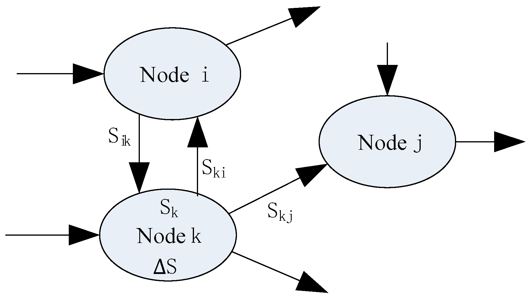
The IO model has been widely used for quantitative analysis of carbon emissions transferred between regions [20,21,22]. Considering the specialness of electric energy transmission, the IO model was improved to the “quasi-input-output (QIO)” model in the literature [19,23]. The latter can track the electric energy and the specific carbon emissions from power plants to users through all the transmission paths in the network. The model is very suitable for calculating the carbon EFs and the carbon emissions. Take the transmission lines, the substations, and the distribution networks as accounting nodes, as illustrated in Figure 1. Owing to the interconnectedness of the power grid, a node may receive electric energy from multiple nodes and transmit electric energy to multiple nodes at the same time. In the QIO model, the total inflow electric energy of a node is equal to the sum of its internal losses and the total outflow electric energy.
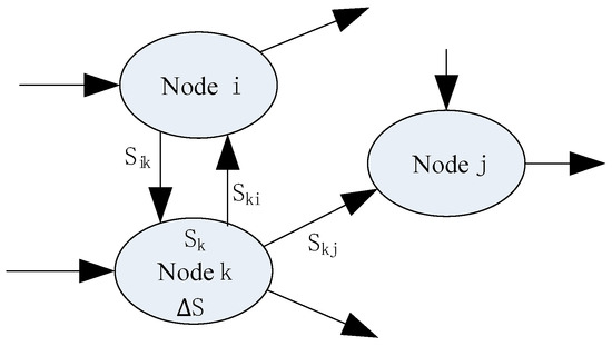
Figure 1.
QIO model for nodes in the grid.
In Figure 1, there are three nodes, namely , , and , with the node being the analytical object. Let the number of branches flowing electric energy into the node be and its outflow branches be . Let the total inflow electric energy of the node k be ; stands for the electric energy flowing from the node to the node ; represents the electric energy flowing from the node to the node ; means the electric energy consumed internally in the node . The QIO model for the node is:
According to the balance principle of carbon emissions, the carbon emissions of the node are equal to the sum of carbon emissions flowing into the node and also equal to the sum of the carbon emissions of the losses within the node and the total carbon emissions flowing out of the node, which is shown as:
In Equation (2), stands for the total carbon emissions of the node , represents the carbon emissions flowing from the node to the node , is the carbon emissions flowing from the node to the node , and is the carbon emissions generated by the internal losses of the node .
3. Dynamic Accounting Method for Carbon Emissions on the Grid Side
3.1. Electric Energy Metering Network
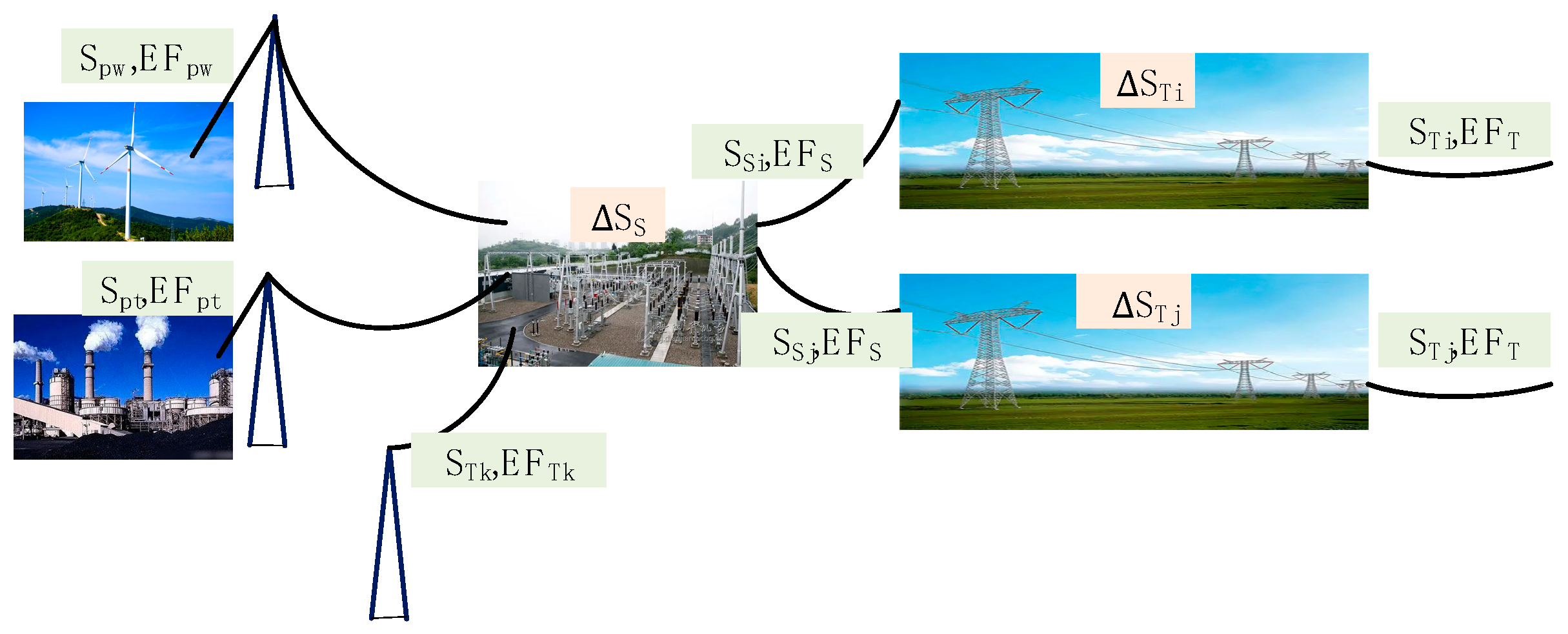
In the power system, the electric energy produced by power plants flows from the transmission lines into the substations at all levels of the distribution network and then onto the user side. Figure 2 shows a simple power network that includes the basic links such as the power plants for multiple forms of energy, the transmission lines, the substations, and the distribution networks. In each link, metering devices are provided for electric energy measurement or monitoring.
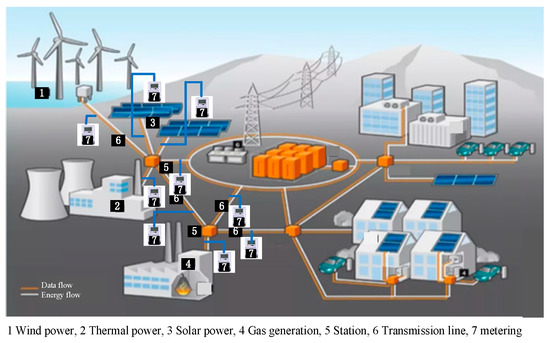
Figure 2.
Electric energy measuring points in the power grid.
As can be seen in Figure 2, the electric energy produced by the power plant is transmitted to the substation for voltage conversion. The substation can connect to the lines from multiple power plants or multiple forms of energy sources for energy interconnection. Electricity is then transmitted to the distribution network along transmission lines. The carbon emission generated by the power plant is transmitted outward through the electricity flow path, which can be calculated by direct measurement or LCA. Therefore, the carbon emission factors of the power plants are equivalent to what is known.
The calculation of carbon emissions is a complicated process due to the interconnectedness of the power grid. On the one hand, electricity is converted from multiple forms of energy with different carbon emission factors. On the other hand, the energy structure is always changing. For instance, new energy sources such as photovoltaic and wind power are dependent on the weather and the season and thus are dynamic in space and time. Using a single average EF for carbon emission accounting cannot truly reflect the real carbon emissions on the grid side.
3.2. Dynamic Carbon Emission Accounting Method on the Grid Side
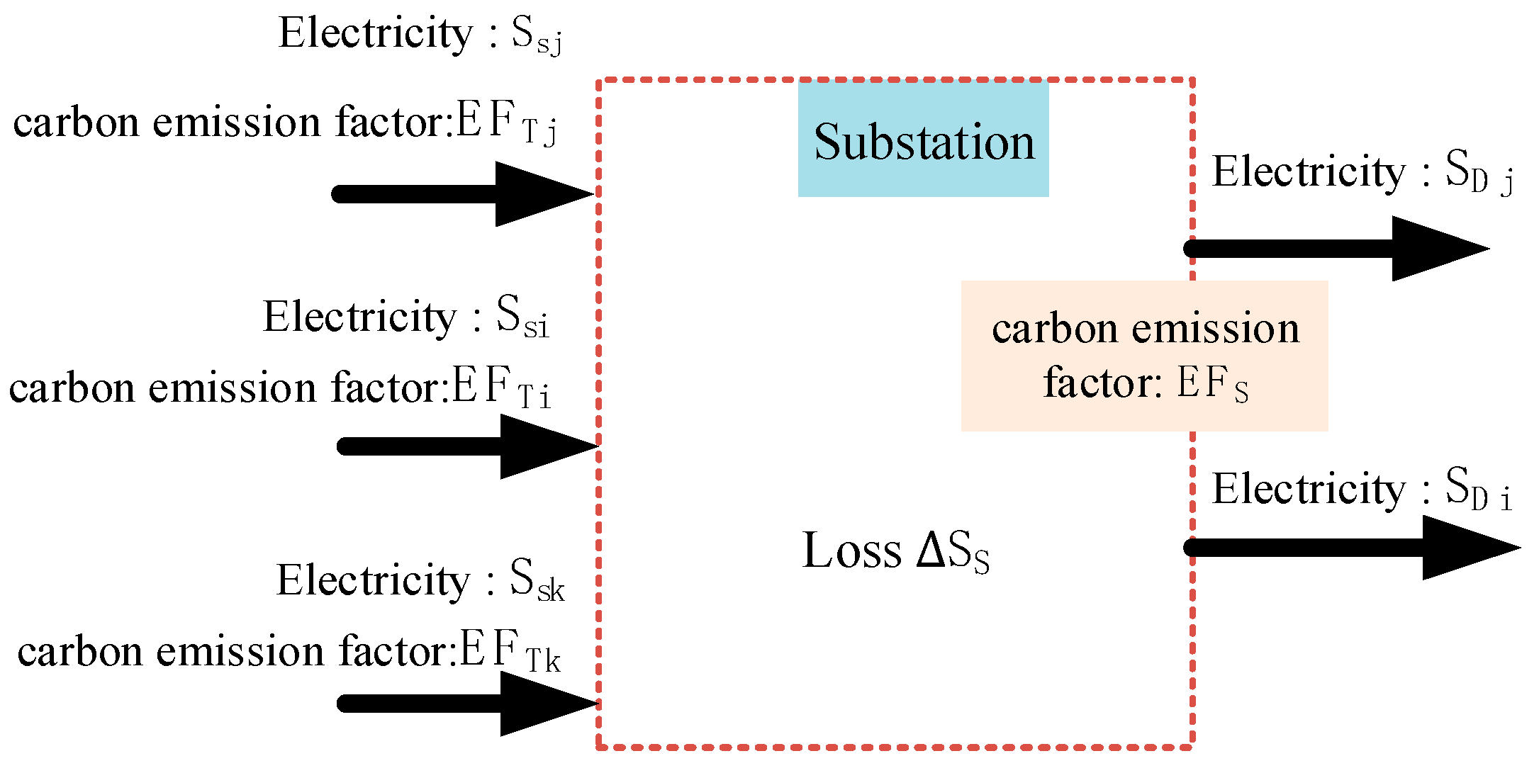
It can be seen from the distribution of the metering devices in Figure 2 that all the inflow and outflow electricity of the grid nodes can be acquired by reading the data uploaded from the metering devices. Take the nodes as carbon emission accounting boundaries. When the carbon EFs of the inflow electricity are known, the total carbon emissions of the nodes can be calculated by multiplying the electricity data by the carbon EF on the input side, and then the carbon EFs of the outflow electricity can be calculated based on the balance principle of carbon emissions. Based on what has been mentioned above, the dynamic carbon emission accounting model on the grid side is shown in Figure 3.

Figure 3.
Carbon emission accounting model on the grid side.
In addition to voltage transformation, substations are also important hubs for grid interconnection, interconnecting different transmission lines, and completing energy exchange and trade. Taking the substation nodes as the accounting boundary is a comprehensive carbon emission accounting model when there are multiple sources of inflow electricity and branches of outflow electricity, as shown in Figure 4.
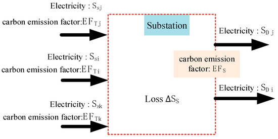
Figure 4.
Carbon emission accounting model for nodes in substations.
In Figure 4, suppose the electricity from three different sources (different power plants and perhaps different primary energies) flowing into the node of the substation are , , and , and the corresponding carbon emission factors are , , and . , , and are read from the energy metering devices, and their time resolutions are determined by the update frequency of the metering devices. , , and are calculated from the prior nodes. They are equal to the carbon EFs of the power plant if the prior node is directly connected to the power plant, or the carbon EFs of the outflow electricity of the prior node can be calculated according to the calculation method in this section.
According to Equation (2), the total carbon emissions flowing into the node are:
The carbon emissions, including the internal losses and the outflow electricity, are calculated by adding all the electricity flowing into the node. Therefore, the internal losses and the outflow electricity of the node should bear the same carbon emission factor. The carbon emission factor of the substation node is:
The carbon emissions generated by the internal losses of the node and the outflow of electricity are:
The above calculation process is based on electric energy metering data. When the carbon EF of the outflow electricity on the power generation side is known, the total carbon emissions, the carbon emissions generated by internal losses, the carbon emissions flowing out of the nodes, and the EFs of the nodes on each link of the transmission line, the substation, and the distribution side can be calculated step by step. The time resolution of the carbon accounting results depends on the update frequency of the electric energy metering devices; thus, the carbon emission accounting results are dynamic in the time dimension. The accounting boundary is no longer limited to regions but to nodes; thus, the results are flexible in the spatial dimension.
4. Case Validation
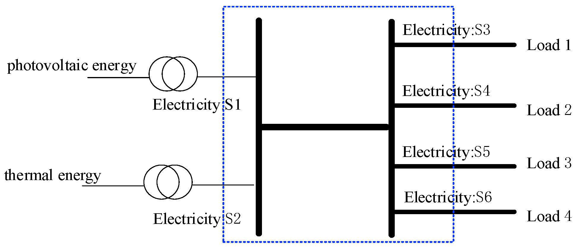
Taking a 110 kV substation in Figure 5 as a carbon emission accounting case, inflow electricity includes a photovoltaic power station and a fossil-fuel power station, and outflows to four different loads. Taking the substation as a carbon emission accounting node, the inflow energy from the photovoltaic power station is S1, the inflow energy from the fossil-fuel power station is S2, and the outflow electricity to the four loads is S3, S4, S5, and S6, respectively.
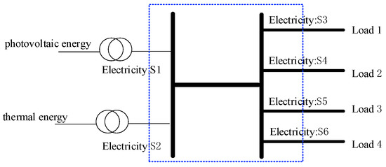
Figure 5.
Schematic diagram of the input and output lines of a substation.
The inflow electricity and load electricity of the node were recorded by hour for carbon emission accounting and analysis on a certain day in March, as shown in Table 1.

Table 1.
Inflow and outflow of electricity at the substation on a certain day in March.
Table 2 shows the carbon EFs of the power generation side from LCA for various forms of energy.

Table 2.
Carbon emission factors from LCA.
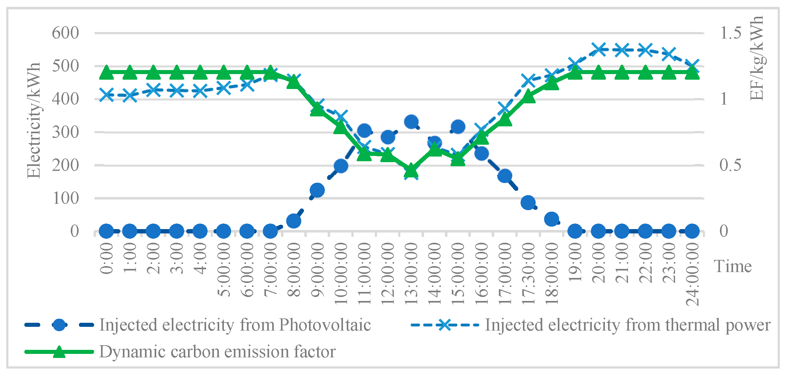
The carbon EFs and the amount of carbon emissions from the substation were calculated using Equations (3)–(6) in Section 3.2. Figure 6 shows the relationship between the carbon EFs and the inflow of electricity over time.
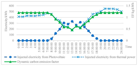
Figure 6.
The curve of inflow electricity and dynamic carbon emission factors.
As seen in Figure 6, during the period from 18:00 to 8:00, there was no inflow of electricity from the photovoltaic power plant, and all the loads were powered by thermal power. The carbon EF remained unchanged and was equal to that of thermal power. During the period from 8:00 to 18:00, as photovoltaic power stations began to generate electricity, the injected photovoltaic electricity increased. This reduced the demand for thermal power generation, resulting in a decrease in EFs. The carbon EFs were constantly changing over time due to the inflow of photovoltaic electricity.
According to the average carbon EF of 0.5703 t CO2/MWh for the power grid in 2022 released by the Ministry of Ecology and Environment of China, the total carbon emissions are 7.4042 t CO2. The carbon emissions calculated by the carbon emission accounting method proposed in this study are 12.932 t CO2. There is a significant difference between the two accounting results. For this substation, the total injected photovoltaic electricity accounts for a relatively small proportion, but the calculation results using the annual average EF did not judge this actual situation. The results calculated using the method presented in this study are more in line with the actual situation and well reflect the changes in carbon emissions over time.
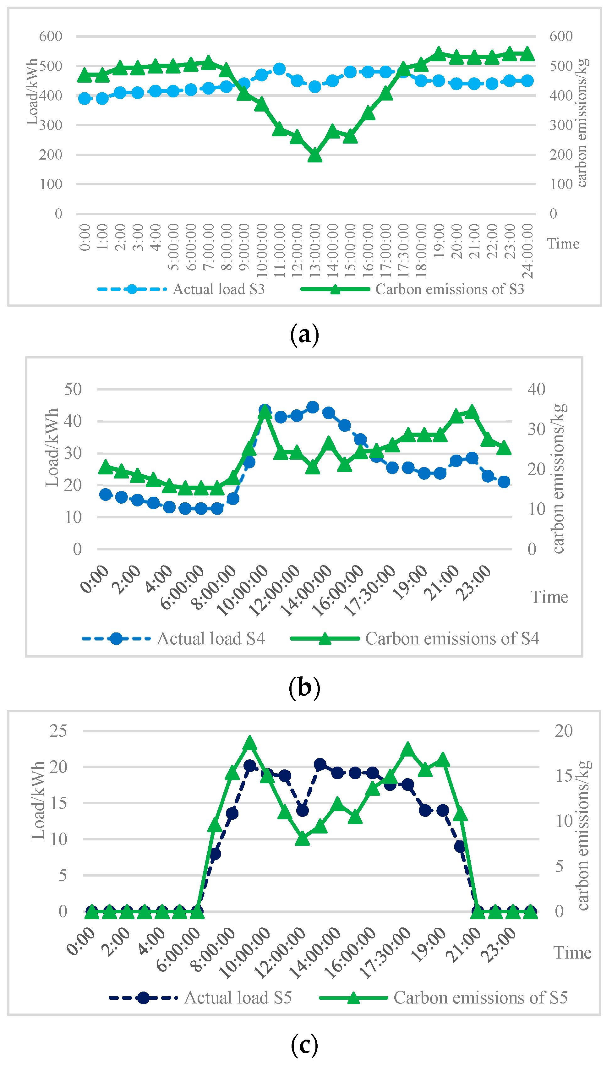
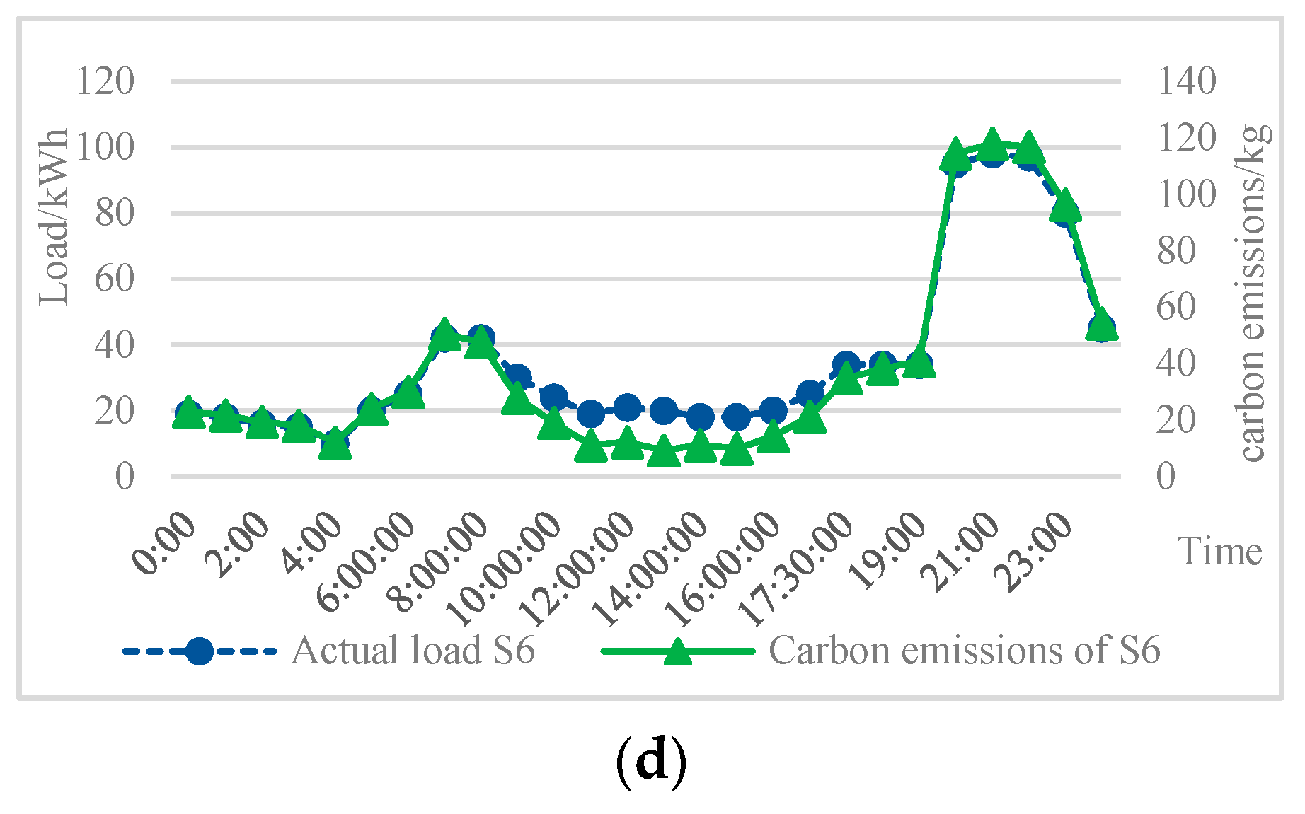
The correlation curve of the carbon emissions and the load of each outflow branch is shown in Figure 7.
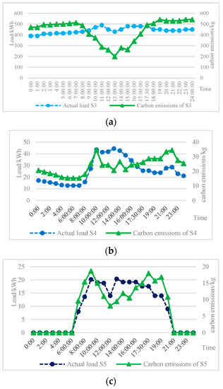

Figure 7.
The correlation curve of the load and the carbon emissions of output branches (a) Dynamic variation curve of load S3 and carbon emissions. (b) Dynamic variation curve of load S3 and carbon emissions. (c) Dynamic variation curve of load S3 and carbon emissions. (d) Dynamic variation curve of load S3 and carbon emissions.
From Figure 7, during the period from 18:00 to 8:00, the carbon emissions of each load are proportional to the load as there is only an inflow of thermal power. During the period from 8:00 to 18:00, the carbon emissions of each load decrease because of the inflow of photovoltaic electricity. This shows that carbon emissions change over time and that clean energy does play a role in carbon emission reduction, which is conducive to enhancing consumers’ awareness of carbon reduction.
5. Discussion and Conclusion
Based on the concept of carbon flow and the QIO model, the accounting model of carbon emissions on the power grid side was established in this study, and the conclusions are as follows:
- (1)
- Uncertainty analysis
The data sources for the carbon emission accounting model in this study include LCA electricity carbon EFs and electricity metering data. Therefore, the total uncertainty of the calculation results of the model is:
In Formula (7), is the uncertainty of the carbon EF of LCA power, and the uncertainty of LCA calculated using data from China Electricity Union in reference [24] is 6.36%. is the uncertainty of the electric metering devices, and the uncertainty of 0.2-level electric metering devices is 0.2%. Therefore, the total uncertainty of the carbon accounting results in this study is 6.36%.
- (2)
- The carbon EFs, the amount of carbon emissions generated by the internal losses of the nodes, and the carbon emissions flowing out of the nodes can be calculated over time using the electric metering data, taking the nodes as accounting boundaries such as transmission lines, substations, and distribution sides. The accounting method is simple and clear.
- (3)
- This accounting model is dynamic in the spatiotemporal dimensions, as it covers all the nodes on the power grid side in the spatial dimension and shares the same time resolution with the electric energy measurement data in the temporal dimension.
- (4)
- Next, we will rely on the electricity metering platform of Southern Power Grid and select a small power grid for carbon emission accounting, providing experience for future promotion across the entire network.
Author Contributions
Conceptualization, H.H. and X.X.; methodology, S.Z.; validation, L.Z. and W.Z.; formal analysis, X.X.; investigation, X.X.; resources, H.H.; data curation, L.Z.; writing—original draft preparation, X.X.; writing—review and editing, H.H. and X.X.; supervision, S.Z.; project administration, X.X.; funding acquisition, S.Z. All authors have read and agreed to the published version of the manuscript.
Funding
This research was funded by Digital Grid Research Institute, China Southern Power Grid (grant number 670000KK52210037), and Guangdong Provincial Key Laboratory of Digital Grid Technology.
Data Availability Statement
The data used in the study comes from the measurement platform of China Southern Power Grid.
Acknowledgments
This work was financially supported by the Digital Grid Research Institute and the China Southern Power Grid.
Conflicts of Interest
The authors declare no conflict of interest.
References
- Nabavi, S.A.; Motlagh, N.H.; Zaidan, M.A.; Aslani, A.; Zakeri, B. Deep learning in energy modeling: Application in smart buildings with distributed energy generation. IEEE Access 2021, 9, 125439–125461. [Google Scholar] [CrossRef]
- Li, Y.; Zhang, N.; Du, E.; Liu, Y.; Cai, X.; He, D. Research and Benefit Analysis of Low-carbon Demand Response Mechanism in Power System Based on Carbon Emission Flow. Chin. J. Electr. Eng. 2022, 42, 2830–2842. [Google Scholar]
- Kopsakangas-Savolainen, M.; Mattinen, M.K.; Manninen, K.; Nissinen, A. Hourly-based greenhouse gas emissions of electricity-cases demonstrating possibilities for households and companies to de-crease their emissions. J. Clean. Prod. 2017, 153, 384–396. [Google Scholar] [CrossRef]
- Li, Y.; Zhang, N.; Du, E.; Liu, Y. Mechanism study and benefit analysis on power system low carbon demand response based on carbon emission flow. Proc. CSEE 2022, 42, 2830–2842. [Google Scholar]
- Eggleston, H.S.; Buendia, L.; Miwa, K.; Ngara, T.; Tanabe, K. 2006 IPCC Guidelines for National Greenhouse Gas Inventories; IPCC National Greenhouse Gas Inventories Programme: Geneva, Switzerland, 2006. [Google Scholar]
- Miller, G.J.; Novan, K.; Jenn, A. Hourly accounting of carbon emissions from electricity consumption. Environ. Res. Lett. 2022, 17, 044073. [Google Scholar] [CrossRef]
- Duan, S.; Chen, H.; Zheng, X.; Huang, J.; Deng, S. Bidding strategy of electricity generation and electricity market equilibrium analysis under the background of carbon market. Electr. Meas. Instrum. 2022, 59, 33–41. [Google Scholar]
- Tranberg, B.; Corradi, O.; Lajoie, B.; Gibon, T.; Staffell, I.; Andresen, G.B. Real-time carbon accounting method for the European electricity markets. Energy Strategy Rev. 2019, 26, 100367. [Google Scholar] [CrossRef]
- Clauß, J.; Stinner, S.; Solli, C.; Lindberg, K.B.; Madsen, H.; Georges, L. Evaluation Method for the Hourly Average CO2eq. Intensity of the Electricity Mix and Its Application to the Demand Response of Residential Heating. Energies 2019, 12, 1345. [Google Scholar] [CrossRef]
- Zhou, T.; Kang, C.; Xu, Q. Preliminary Theoretical Investigation on Power System Carbon Emission Flow. Autom. Power System. 2012, 36, 38–44. [Google Scholar]
- Kang, C.; Cheng, Y.; Sun, Y. Recursive Calculation Method of Carbon Emission Flow in Power Systems. Autom. Power Syst. 2017, 41, 10–16. [Google Scholar]
- Chen, D.; Xian, W.; Wu, T. Allocation of Carbon Emission Flow in Hybrid Electricity Market. Power Syst. Technol. 2016, 40, 1683–1688. [Google Scholar]
- Minx, J.C.; Wiedmann, T.; Wood, R.; Peters, G.P.; Lenzen, M.; Owen, A.; Scott, K.; Barrett, J.; Hubacek, K.; Baiocchi, G.; et al. Input−output analysis and carbon footprinting: An overview of applications. Econ. Syst. Res. 2009, 21, 187–216. [Google Scholar] [CrossRef]
- Leontief, W.; Ford, D. Air pollution and the economic structure: Empirical results of input−output calculations. In Proceedings of the Fifth International Conference on Input−Output Techniques; North Holland Pub. Co.: Geneva, Switzerland, 1971. [Google Scholar]
- Praseeda, K.I.; Reddy, B.V.V.; Mani, M. Embodied energy assessment of building materials in India using process and input−output analysis. Energy Build. 2015, 86, 677–686. [Google Scholar] [CrossRef]
- Chen, G.; Guo, S.; Shao, L.; Li, J.; Chen, Z.-M. Three-scale input−output modeling for urban economy: Carbon emission by Beijing 2007. Commun. Nonlinear Sci. Numer. Simul. 2013, 18, 2493–2506. [Google Scholar] [CrossRef]
- Su, B.; Ang, B.W. Input−output analysis of CO2 emissions embodied in trade: A multi-region model for China. Appl. Energy 2014, 114, 377–384. [Google Scholar] [CrossRef]
- Machado, G.; Schaeffer, R.; Worrell, E. Energy and carbon embodied in the international trade of Brazil: An input−output approach. Ecol. Econ. 2001, 39, 409–424. [Google Scholar] [CrossRef]
- Qu, S.; Wang, H.; Liang, S.; Shapiro, A.M.; Suh, S.; Sheldon, S.; Zik, O.; Fang, H.; Xu, M. A Quasi-Input-Output model to improve the estimation of emission factors for purchased electricity from interconnected grids. Appl. Energy 2017, 200, 249–259. [Google Scholar] [CrossRef]
- Kanemoto, K.; Moran, D.; Hertwich, E.G. Mapping the carbon footprint of nations. Environ. Sci. Technol. 2016, 50, 10512–10517. [Google Scholar] [CrossRef]
- Tukker, A.; Bulavskaya, T.; Giljum, S.; De Koning, A.; Lutter, S.; Simas, M.; Stadler, K.; Wood, R. The global resource footprint of nations. Carbon, water, land and materials embodied in trade and final consumption. In A Publication of the Compiling and Refining of Economic and Environmental Accounts Project; The Netherlands Organization for Applied Scientific Research – NL-2628 XE Delft; Leiden University: Leiden, The Netherlands, 2014. [Google Scholar]
- Chen, S.; Chen, B. Tracking inter-regional carbon flows: A hybrid network model. Environ. Sci. Technol. 2016, 50, 4731–4741. [Google Scholar] [CrossRef]
- Kodra, E.; Sheldon, S.; Dolen, R.; Zik, O. The North American electric grid as an exchange network: An approach for evaluating energy resource composition and greenhouse gas mitigation. Environ. Sci. Technol. 2015, 49, 13692–13698. [Google Scholar] [CrossRef]
- Huang, N.; Wang, H.T.; Fan, C.D.; Zhou, S.C.; Hou, P.; Yang, J. LCA data quality assessment and control based on uncertainty and sensitivity analysis. Acta Sci. Circumstantiae 2012, 32, 1529–1536. [Google Scholar]
Disclaimer/Publisher’s Note: The statements, opinions and data contained in all publications are solely those of the individual author(s) and contributor(s) and not of MDPI and/or the editor(s). MDPI and/or the editor(s) disclaim responsibility for any injury to people or property resulting from any ideas, methods, instructions or products referred to in the content. |
© 2023 by the authors. Licensee MDPI, Basel, Switzerland. This article is an open access article distributed under the terms and conditions of the Creative Commons Attribution (CC BY) license (https://creativecommons.org/licenses/by/4.0/).

