Practical Energy Management Control of Fuel Cell Hybrid Electric Vehicles Using Artificial-Intelligence-Based Flatness Theory

Abstract

This paper proposes a practical solution to address the energy management issue in fuel cell hybrid electric vehicles (FCHEVs). This solution revolves around a powertrain system that contains a fuel cell (FC) as the main supply, a photovoltaic cell (PC) as the secondary energy source, and a battery bank (Batt) as backup storage to compensate for the FC’s low response rate. The energy in this hybrid powertrain system alternated between the designated elements and the load via a DC bus, and to maintain a stable output voltage, the DC link was adjusted using a nonlinear approach that is based on the flatness theory and the nonlinear autoregressive moving average (NARMA-L2) neuro-controller. As for the current regulation loops, the sliding mode technique was employed to attain the high dynamic of the reference signals produced by the energy manager loop. To validate the accuracy of the proposed energy management approach (EMA), a test bench was equipped with digital, electronic circuits and a dSPACE DS-1104 unit. This experimental bench contained a fuel cell emulator FC of 1200 W and 46 A, lithium-ion batteries of 24 V, and a solar source capable of 400 W. The obtained results, indeed, attested to the validity of the approach used, yielding a notable performance during multiple charge variations. This ultimately demonstrated that the management approach enhanced the efficiency of the hybrid powertrain.

1. Introduction

The use of renewable energy sources, such as fuel cells and solar cells, to operate electric motors has increased in recent years [1,2,3,4,5,6], which has paved the way for the development of modern electric vehicles (EV). Nowadays, researchers specializing in vehicle technologies have the sole aim of piloting their plans independent from fossil energies. To accomplish this, a recommended procedure is the use of a hybrid renewable source in combination with different storage systems, i.e., super capacitors or batteries, which do not run on gasoline or diesel fuel and which do not release carbon dioxide (CO₂). On the one hand, the FC supply source has largely been used in the electrical transport sector [7,8,9,10] owing to its energy-efficient and non-polluting features; on the other hand, certain characteristic issues can hinder its performance, such as the slow dynamicity of the energetic process. This is why such systems can be equipped with solar cells and storage devices to support the main energy source in order to meet the necessary load power, especially in the case of electric vehicles and particularly during times of the day with intense sunlight. Moreover, this proposal comes in parallel with distinct progress in the efficiency of solar cells [11,12,13], the usage of which to run electric vehicles can be considered a motivating factor that helps to advertise such a modern mode of transportation in the global markets, highlighting several economic and technical advantages of such applications [14,15].

Furthermore, the utilization of solar cells may reduce the aesthetics of plug-in electric vehicles; however, it permits electric car owners to receive lower bills concerning the recharging of batteries or hydrogen and to avoid an excessive load demand in modern smart grids, especially in areas with intense sunlight.

As long as the amount of power produced through solar energy fluctuates over a certain well-defined period, it cannot be considered as a progressive power generator. This is why devices depending on solar energy are coupled with chemical accumulators, such as batteries, to ensure the instantaneousness of energy storage. Furthermore, the existence of several sources of different natures reinforces the reliability and the efficiency of such systems [16,17,18]. In order to properly manage these hybrid systems in an EV, it is vital that robust and efficient control approaches are implemented whilst maintaining the high performance of the powertrain.

Recently, a noteworthy level of attention has been directed towards EMAs in several renewable applications [19,20,21]. Numerous publications have documented energy management strategies. For instance, PID controllers and fuzzy logic are discussed in [22]. Bourbon et al. [23] provided a comparative study between the linear programming and the heuristic methods. An EV application using an optimized management strategy was described in [24], a predictive controller was used in [25], Xie et al. [26] studied an artificial neural network, and lastly, adaptive and optimal control methodologies were studied in [27,28].

An exhaustive and interesting strategy to address the energy management issue was established based on the nonlinear differential flatness model. This is a relatively recent concept in EMAs studies [29,30,31]; however, it has been studied and actively improved since 1992, formulated by Fliess et al. [32]. The major advantage of this approach is the parameterization of the dynamic behavior in physical systems. Thus, it is founded on the description of a set of fundamental variables representing the flat outputs. The first phases of flatness control implementation involve the utilization of the desired trajectory that is suitable for the system’s model; then, the strategy involves the usage of a control conception through a regulation loop that ensures the trajectory tracking. Additionally, using this approach without including any differential equations, the trajectories of the model are completely predictable based on the state of its flat outputs and its derivative, which fulfils the main purpose of this strategy.

Nevertheless, there still exist a few impediments to the flatness theory that should be addressed, particularly in EV applications, such as cases when fast variations in the power demand of the motor (acceleration or braking) occur, causing a significant perturbation error in the output voltage of the DC link [30,31]. To resolve this issue and to preserve a stable DC voltage, such a system must follow an efficient control scheme. Therefore, this paper proposes a strategy that employs a hybrid control scheme consisting of flatness and a neuro-controller based on the nonlinear autoregressive moving average to enhance the DC bus output voltage and improve the performance of the energy manager.

To date, the artificial neural networks in the control domain of dynamic nonlinear systems have witnessed significant success [33,34,35]. The NARMA-L2 is one of the most prominent among the ANN approaches due to its implementation simplicity and offline training, referring to its ability to approximate the nonlinear functions. Theoretically, this type of neuro-controller does not necessitate a precise mathematical description of the model to be controlled [36,37].

Contributions of the Study

In this paper, the NARMA-L2 controller is applied to pursue the trajectory of the DC bus energy and to improve the performance of the energy manager based on the flatness theory. The flat controller uses two regulation loops; the first is intended for DC bus regulation (which is improved with a NARMA-L2 artificial intelligence system), and the second loop is intended for energy management between the different generated powers. The results presented below show that the hybridization between the differential flatness and the ANN (NARMA-L2) successfully reduces the load perturbation error in the DC link response signals and increases the efficiency of the EMA, giving it a high power dynamicity and precise voltage. The employment of solar cells can improve energy efficiency and decrease reliance on fuel cells and batteries in a novel design that will undoubtedly shorten charging times and decrease the size of the hydrogen storage tank. The addition of (PC) to electric vehicles can potentially increase their driving distance.

2. System under Study and Mathematical Modelling

2.1. Hybrid System and Power Converter Description

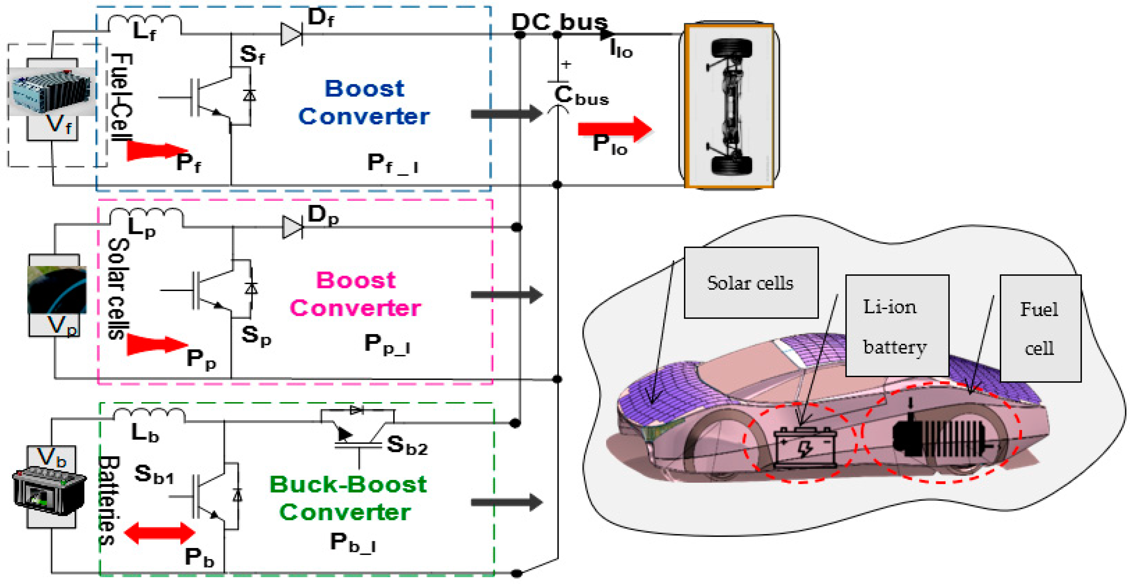
A fuel cell, solar cells, and Li-ion batteries are used in the proposed hybrid power system to supply the EV motor. Correspondingly, the system must contain boost and buck-boost converters along with a control unit. A basic design of this proposed hybrid system is presented in Figure 1, and the equations demonstrating the boost converters with the small signals model are determined.

To establish the mathematical model of the power converters, some hypotheses are formulated, supposing that the components are ideal and lossless and that the converters operate in a continuous conduction mode (CCM). With the ideal hypothesis V_dc = V_out, it is deduced that one variable can replace the other, taking into consideration that V_out is the output voltage in the boost converters. The state equations for the switching cycle in the boost converters are demonstrated in Equations (1) and (2):

$${\mathrm{L}}_{\mathrm{n}}\frac{{\mathrm{di}}_{\mathrm{L}\_\mathrm{n}}}{\mathrm{dt}}={\mathrm{V}}_{\mathrm{in}\_\mathrm{n}}-\left(1-{\mathrm{d}}_{\mathrm{n}}\right){\mathrm{V}}_{\mathrm{dc}}$$

(1)

$${\mathrm{C}}_{\mathrm{dc}}\frac{{\mathrm{dV}}_{\mathrm{dc}}}{\mathrm{dt}}=\left(1-{\mathrm{d}}_{\mathrm{n}}\right){\mathrm{i}}_{\mathrm{L}\_\mathrm{n}}-{\mathrm{I}}_{\mathrm{load}}$$

(2)

To explain the equation further, n = [fc, s], that is, in accordance with the fuel cell and solar cell boost converters. Vdc is the measured DC bus voltage. V_{in_n} is the fuel cell or solar cell voltage. d_n is the duty cycle of the switches in each converter. i_{L_n} is the inductor current of the boost phases. iLoad is the load current. C_dc is the capacitance value of the DC bus. To display the disturbance in the state variables, Equations (3)–(5) are used:

$$i_{L\_n}=I_{L\_n}+{\widehat{i}}_{L\_n} V_{in\_n}=V_{in\_n}+{\widehat{v}}_{in\_n} d_n=D_n+{\widehat{d}}_n$$

(3)

$${\mathrm{C}}_{\mathrm{d}\mathrm{c}}\frac{\mathrm{d}({\mathrm{V}}_{\mathrm{d}\mathrm{c}}+{\widehat{\mathrm{v}}}_{\mathrm{d}\mathrm{c}})}{\mathrm{d}\mathrm{t}}=(1-{\mathrm{D}}_{\mathrm{n}}-{\widehat{\mathrm{d}}}_{\mathrm{n}})({\mathrm{I}}_{\mathrm{L}\_\mathrm{n}}+{\widehat{\mathrm{i}}}_{\mathrm{L}\_\mathrm{n}})-({\mathrm{I}}_{\mathrm{l}\mathrm{o}\mathrm{a}\mathrm{d}}+{\widehat{\mathrm{i}}}_{\mathrm{l}\mathrm{o}\mathrm{a}\mathrm{d}})$$

(4)

$${\mathrm{L}}_{\mathrm{n}}\frac{\mathrm{d}({\mathrm{I}}_{\mathrm{L}\_\mathrm{n}}+{\widehat{\mathrm{i}}}_{\mathrm{L}\_\mathrm{n}})}{\mathrm{d}\mathrm{t}}=({\mathrm{V}}_{\mathrm{i}\mathrm{n}\_\mathrm{n}}+{\widehat{\mathrm{v}}}_{\mathrm{i}\mathrm{n}\_\mathrm{n}})-(1-{\mathrm{D}}_{\mathrm{n}}-{\widehat{\mathrm{d}}}_{\mathrm{n}})({\mathrm{V}}_{\mathrm{d}\mathrm{c}}+{\widehat{\mathrm{v}}}_{\mathrm{d}\mathrm{c}})$$

(5)

${\widehat{i}}_{L\_n},{\widehat{v}}_{in\_n},{\widehat{d}}_n,{\widehat{v}}_{dc},{\widehat{i}}_{load}$ are the disturbance variables of the small signals model.

Through the transition to the Laplace transformation and then towards the matrix mode, the state variables of the used boost converters are presented in Equation (6):

$$\left[\begin{array}{l}{\widehat{\mathrm{i}}}_{\mathrm{L}\_\mathrm{n}}(\mathrm{s})\\ {\widehat{\mathrm{v}}}_{\mathrm{d}\mathrm{c}\_\mathrm{n}}(\mathrm{s})\end{array}\right]={\left[\begin{array}{cc}\mathrm{s}{\mathrm{L}}_{\mathrm{n}}& 1-{\mathrm{D}}_{\mathrm{n}}\\ 1-{\mathrm{D}}_{\mathrm{n}}& -(\mathrm{s}{\mathrm{C}}_{\mathrm{d}\mathrm{c}}+\frac{{\widehat{\mathrm{i}}}_{\mathrm{l}\mathrm{o}\mathrm{a}\mathrm{d}}(\mathrm{s})}{{\widehat{\mathrm{v}}}_{\mathrm{i}\mathrm{n}}(\mathrm{s})})\end{array}\right]}^{-1}.\left[\begin{array}{l}{\mathrm{V}}_{\mathrm{d}\mathrm{c}}\\ {\mathrm{I}}_{\mathrm{L}\_\mathrm{n}}\end{array}\right].{\widehat{\mathrm{d}}}_{\mathrm{n}}(\mathrm{s})+{\left[\begin{array}{cc}\mathrm{s}{\mathrm{L}}_{\mathrm{n}}& 1-{\mathrm{D}}_{\mathrm{n}}\\ 1-{\mathrm{D}}_{\mathrm{n}}& -(\mathrm{s}{\mathrm{C}}_{\mathrm{d}\mathrm{c}}+\frac{{\widehat{\mathrm{i}}}_{\mathrm{l}\mathrm{o}\mathrm{a}\mathrm{d}}(\mathrm{s})}{{\widehat{\mathrm{v}}}_{\mathrm{i}\mathrm{n}}(\mathrm{s})})\end{array}\right]}^{-1}.\left[\begin{array}{l}1\\ 0\end{array}\right].{\widehat{\mathrm{v}}}_{\mathrm{i}\mathrm{n}\_\mathrm{n}}(\mathrm{s})$$

(6)

This shows that the transfer function, which is used for the control signals at the output voltage, can be described in Equation (7):

$${\mathrm{G}}_{\mathrm{v}(\mathrm{s})}=\frac{{\widehat{\mathrm{v}}}_{\mathrm{d}\mathrm{c}}(\mathrm{s})}{{\widehat{\mathrm{i}}}_{\mathrm{L}\_\mathrm{n}}(\mathrm{s})}=\frac{(1-{\mathrm{D}}_{\mathrm{n}}).{\mathrm{V}}_{\mathrm{d}\mathrm{c}}-({\mathrm{L}}_{\mathrm{n}}{\mathrm{I}}_{\mathrm{L}\_\mathrm{n}})\mathrm{s}}{({\mathrm{C}}_{\mathrm{d}\mathrm{c}}{\mathrm{V}}_{\mathrm{d}\mathrm{c}})\mathrm{s}+2(1-{\mathrm{D}}_{\mathrm{n}}){\mathrm{I}}_{\mathrm{L}\_\mathrm{n}}}$$

(7)

In addition, the transfer function for the control signals at the input current is determined as:

$${\mathrm{H}}_{\mathrm{i}(\mathrm{s})}=\frac{{\widehat{\mathrm{i}}}_{\mathrm{L}\_\mathrm{n}}(\mathrm{s})}{{\widehat{\mathrm{d}}}_{\mathrm{n}}(\mathrm{s})}=\frac{({\mathrm{C}}_{\mathrm{d}\mathrm{c}}{\mathrm{V}}_{\mathrm{d}\mathrm{c}})\mathrm{s}+2(1-{\mathrm{D}}_{\mathrm{n}}).{\mathrm{I}}_{\mathrm{L}\_\mathrm{n}}}{({\mathrm{L}}_{\mathrm{n}}{\mathrm{C}}_{\mathrm{d}\mathrm{c}}){\mathrm{s}}^2+{\mathrm{L}}_{\mathrm{n}}\frac{{\widehat{\mathrm{i}}}_{\mathrm{l}\mathrm{o}\mathrm{a}\mathrm{d}}(\mathrm{s})}{{\widehat{\mathrm{v}}}_{\mathrm{d}\mathrm{c}}(\mathrm{s})}\mathrm{s}+{(1-{\mathrm{D}}_{\mathrm{n}})}^2}$$

(8)

The equations representing the associated buck-boost converter are determined using the small signals model, where the switches open and close successively and continuously with a well-defined switching frequency rate.

In other words, when the transistor is “on”, the diode is off, and vice versa. Thus, the input voltage is applied directly to the inductance L, which determines an ascending linear current. The capacitor is discharged in the charging circuit. This is to say that when the transistor is off, the LC filter supplies the load.

The state equations for the switching cycle in the battery buck-boost converter can be expressed as:

$$\{\begin{array}{l}{\mathrm{L}}_{\mathrm{b}}\frac{\mathrm{d}{\widehat{\mathrm{i}}}_{\mathrm{L}\_\mathrm{b}}}{\mathrm{d}\mathrm{t}}={\mathrm{D}}_{\mathrm{b}}.{\widehat{\mathrm{v}}}_{\mathrm{b}}-(1-{\mathrm{D}}_{\mathrm{b}}).{\widehat{\mathrm{v}}}_{\mathrm{d}\mathrm{c}}+{\mathrm{V}}_{\mathrm{d}\mathrm{c}}.{\widehat{\mathrm{d}}}_{\mathrm{b}}\\ {\mathrm{C}}_{\mathrm{d}\mathrm{c}}\frac{\mathrm{d}{\widehat{\mathrm{v}}}_{\mathrm{d}\mathrm{c}}}{\mathrm{d}\mathrm{t}}=-(1-{\mathrm{D}}_{\mathrm{b}}){\widehat{\mathrm{i}}}_{\mathrm{L}\_\mathrm{b}}+{\mathrm{I}}_{\mathrm{L}\_\mathrm{b}}.{\widehat{\mathrm{d}}}_{\mathrm{b}}-\frac{{\widehat{\mathrm{i}}}_{\mathrm{l}\mathrm{o}\mathrm{a}\mathrm{d}}(\mathrm{s})}{{\widehat{\mathrm{v}}}_{\mathrm{d}\mathrm{c}}(\mathrm{s})}{\widehat{\mathrm{v}}}_{\mathrm{d}\mathrm{c}}\end{array}$$

(9)

${\widehat{i}}_{L\_b},{\widehat{v}}_b,{\widehat{d}}_b$ represent the inductance current, the generated voltage, and the control signal in small disturbances around their operating points.

Moving towards the matrix mode and the Laplace transformation, the transfer function, from the output voltage to the control signal, is expressed as:

$$\frac{{\widehat{\mathrm{v}}}_{\mathrm{d}\mathrm{c}}(\mathrm{s})}{{\widehat{\mathrm{i}}}_{\mathrm{L}\_\mathrm{n}}(\mathrm{s})}=\frac{{\widehat{\mathrm{v}}}_{\mathrm{d}\mathrm{c}}(\mathrm{s})}{{\widehat{\mathrm{i}}}_{\mathrm{l}\mathrm{o}\mathrm{a}\mathrm{d}}(\mathrm{s})}\frac{(1-{\mathrm{D}}_{\mathrm{n}})}{(1+{\mathrm{D}}_{\mathrm{n}})}.\frac{1-\frac{{\mathrm{D}}_{\mathrm{n}}.{\mathrm{L}}_{\mathrm{n}}}{\frac{{\widehat{\mathrm{v}}}_{\mathrm{d}\mathrm{c}}(\mathrm{s})}{{\widehat{\mathrm{i}}}_{\mathrm{l}\mathrm{o}\mathrm{a}\mathrm{d}}(\mathrm{s})}{(1-{\mathrm{D}}_{\mathrm{n}})}^2}\mathrm{s}}{1+\frac{\frac{{\widehat{\mathrm{v}}}_{\mathrm{d}\mathrm{c}}(\mathrm{s})}{{\widehat{\mathrm{i}}}_{\mathrm{l}\mathrm{o}\mathrm{a}\mathrm{d}}(\mathrm{s})}{\mathrm{C}}_{\mathrm{d}\mathrm{c}}}{(1+{\mathrm{D}}_{\mathrm{n}})}\mathrm{s}}$$

(10)

The fuel cell/solar cell system instantaneously supplies the electric motor with power after each requested power value.

The main energy source is designed to adapt to the operation regime of the EV motor power when the generated power value is superior to the load request due to the slow processing of the FC. As a quick counter, the EMA adjusts the energy to charge the storage system in order to compensate for the slow dynamicity of the FC, especially with respect to acceleration. While the energy created by the FC source is less than the load demand amount, the energy manager forces the solar cells to support the main source in order to counterbalance the load demand. As for the batteries used in the power train system, they are implemented to provide additional power or absorb it in cases of abrupt acceleration or deceleration.

2.2. Fuel Cell Modelling

The characteristics of a proton exchange membrane fuel cell (PEMFC) are often defined by the theoretical no-load voltage ‘E’, the ohmic overvoltage Vohm, the activation overvoltage V_act, and the concentration overvoltage V_conc. A single-cell voltage ‘V_f’ can be represented as:

$${\mathrm{V}}_{\mathrm{f}}=\mathrm{E}-{\mathrm{V}}_{\mathrm{a}\mathrm{c}\mathrm{t}}-{\mathrm{V}}_{\mathrm{o}\mathrm{h}\mathrm{m}}-{\mathrm{V}}_{\mathrm{c}\mathrm{o}\mathrm{n}\mathrm{c}}$$

(11)

The FC thermodynamic potential is given by the term ‘E’, while ‘V_act’ is the voltage drop caused by activation losses. Several models have been developed to validate and analyze the performance, behavior, and design according to the desired objectives. There exist some static models that describe the polarization curve of a static model PEMFC. For instance, the static model of Larminie and Dicks [38] is chosen because of its simplicity of implementation. This FC model is described as:

$$V_{fc}=E_0-\overline{A} \log \left(\frac{i_{FC}-i_n}{i_0}\right)-R_m(i_{FC}-i_n)+\overline{B} \log (1-\frac{i_{FC}-i_n}{i_{Lim}})$$

(12)

i₀ is the exchange current that defines the electrode–electrolyte exchanges in an open circuit. in is the internal current that allows us to take into account a possible gas and/or electron intersectionality through the electrolyte.

A is the Tafel’s constant. R_m is the total resistance of the fuel cell. B is the mass transfer constant. i_FC is the density of the permanent operating current (A/cm²), and i_Lim is the limit current density.

2.3. Battery Modelling

In this study, a Li-ion battery model is used. The pseudo-dynamic model proposed in [39] is also employed. The following equations demonstrate the charge/discharge voltage as a function of the battery current:

$$\{\begin{array}{c}{V}_b\left(i_b\right)=E_0-R.i_b-k\frac{Q}{Q-it}.\left(it+i^{*}\right)+Aexp\left(-B.it\right)\\ V_b\left(i_b\right)=E_0-R.i_b-k\frac{Q}{it-0.1Q}.i^{*}-k\frac{Q}{Q-it}.it+Aexp\left(-B.it\right)\end{array}$$

(13)

2.4. Drivetrain Modelling

The mechanical characteristics required for driving a rolling electrical vehicle can be modelled using the total resistance effort (F_r), which displays the advancement force that the motorization system should overcome.

The Fr function can be written with the following formula:

$$\{\begin{array}{c}{F}_r=F_{roul}+F_{aero}+M.g.p\%+m.\gamma \\ Where: F_{aero}=\frac{1}{2}\times \rho \times v^2\times C_x\times S_f\\ F_{roul}=C_{Rt}.M.g\end{array}$$

(14)

The strength of the air resistance depends on the aero-coefficient C_x, the frontal area of the EV S_f, the square speed v², the density of the air ρ, the total mass M in kg (the EV along with the rest of the components), the gravity acceleration g = 9.81 m·s^–2, the incline of the percentage p%, and finally, the dynamic term of acceleration (m·γ) (γ > 0 for accelerations and γ < 0 for decelerations). Froul is the rolling resistance force, which is linked to the rolling coefficient of the tires C_Rt.

In addition, the resistance torque required to obtain the necessary force of the EV can be given as:

$$C_r=F_r.R_r=\left[\frac{1}{2}\times \rho \times v^2\times C_x\times S_f+C_{Rt}.M.g+M.g.p\%+m.\gamma \right].R_r$$

(15)

R_r is the wheel radius.

The resistant torque is augmented by 20% to take into account the different losses in the transmission system. The final transmission is handled by a reducer belt ration d = 6. The EV motor torque C_e is expressed as:

$$C_e=\frac{Cr}{d.\eta }$$

(16)

$\eta$ is the efficiency of the mechanical transmission system.

The EV motor is selected in accordance with the specifications of the technical conditions chart, where the rated power is calculated using the following formula:

$$\{\begin{array}{c}{P}_{load}=P_e=C_e.{\mathsf{\Omega }}_e\\ {\mathsf{\Omega }}_e=d.{\mathsf{\Omega }}_r\end{array}$$

(17)

${\mathsf{\Omega }}_r$ is the maximum vehicle speed in rad/s or in rpm.

2.5. Solar Cell Modelling

The solar cells are mathematically described using three basic equations [40].

The diode current is defined as:

$$I_D=I_0(e^{\raisebox{1ex}{$V_D$}\!\left/ \!\raisebox{-1ex}{$V_T$}\right.}-1)-I_D+I_{SC}-\frac{V_D}{R_P}-I_{PV}=0$$

(18)

The solar cell voltage can be calculated as: $V_{PVcell}=V_D-R_s{I}_{PV}$.

I_SC, R_s, and R_p represent the solar cell current, series resistance, and parallel resistance.

Lastly, the solar cells’ voltage V_P can be determined with:

$$V_{PV}=N_S{V}_{PVcell}$$

(19)

N_s represents the number of cells connected in series.

3. Control Strategy

To define a control strategy that is suitable for the proposed hybrid system, the following main control aims must be determined:

• The DC bus voltage must be adjusted and regulated instantaneously to allow for continuous variations in the EV motor.
• The power requested by the motor must be satisfied instantly.
• Stability and dynamic performance must be ensured when the system operates in a closed loop to prevent the occurrence of any disturbances or failures in the system.
• The power produced by the hybrid system must be generated in an ordinal plan, starting with the main source (the fuel cell), followed by the secondary source (the solar cells), and finally, the storage batteries.

In this paper, the employed EMA is based on flatness theory characteristics. Flat systems are appropriate in situations such as those discussed above, where a trajectory design is required. The nature of such systems reveals itself when employing its exit variables. Subsequently, it is possible to define the control system and design the desired trajectory of the state variables. In order to achieve an efficient energy manager that is based on the flatness theory, the energetic behavior of the hybrid system must be described. According to [41], the energy status of the DC bus ‘f_dc’ and storage batteries energy ‘f_b’ is written as follows:

$$\{\begin{array}{l}{f}_{dc}=\frac{1}{2}{C}_{dc}{V}_{dc}^2\\ f_b=\frac{1}{2}{C}_b{V}_b^2\end{array}$$

(20)

In the same vein, the total energy ‘f_full’ transferred in the system is presented as:

$$f_{full}=\frac{1}{2}{C}_{dc}{V}_{dc}^2+\frac{1}{2}{C}_b{V}_b^2$$

(21)

Correspondingly, the transmitted power in the DC link ‘P_dc’ may be definite as a function of P_{f_l}, P_{p_l}, P_{b_l}, and P_load, as follows:

$$P_{dc}={\dot{f}}_{dc}=P_{f\_l}+P_{p\_l}+P_{b\_l}-P_{load}$$

(22)

P_{f_l}, P_{p_l}, P_{b_l} represent the power produced by the system, bearing in mind the losses caused by the converters used.

To identify the flatness theorem’s compatibility with the studied hybrid system, it is necessary to ensure that the conditions which are cited in [32] are satisfied. The flatness of a nonlinear physical system can be demonstrated provided that the vector of its output variables ‘f’ is described mathematically taking into account the state variables ‘x’, command variables ‘α’, and a finite number of its derivatives, as follows:

$$\{\begin{array}{l}\dot{x}=h\left(x,\alpha \right)\\ f=\varphi (x,\alpha ,\dot{\alpha },...,{\alpha }^{(n)})\end{array} \mathrm{and} f\in R^m:f=\left[\begin{array}{l}{f}_1\\ f_2\\ .\\ .\\ f_m\end{array}\right]$$

(23)

The vectors ‘x’ and ‘α’ must be expressed as:

$$\{\begin{array}{l}x=\phi (f,\dot{f},...,f^{(j)})\\ \alpha =\psi (f,\dot{f},...,f^{(j+1)})\end{array} \mathrm{and} \alpha \in R^m:\alpha =\left[\begin{array}{l}{\alpha }_1\\ {\alpha }_2\\ .\\ .\\ {\alpha }_m\end{array}\right] ,x\in R^k:x=\left[\begin{array}{l}{x}_1\\ x_2\\ .\\ .\\ x_k\end{array}\right]$$

(24)

Moreover, in this study, the control loops of the associated converters are adjusted through a set of reference currents. The reference signals are then calculated as a function of the reference powers generated by the EMA, so that:

$$P_{fc\_ref}=P_f=I_f.V_f=I_{f\_ref}.V_f$$

(25)

$$P_{p\_ref}=P_p=I_p.V_p=I_{p\_ref}.V_p$$

(26)

$$P_{b\_ref}=P_b=I_b.V_b=I_{b\_ref}.V_b$$

(27)

The power generated by the fuel cell, the solar cells, and the batteries are represented by the values P_fc, P_p, and P_b, respectively. In addition, the power consumed by the EV motor is written as a function of the energy transported through the DC bus, DC link capacitance, and the load current, as described below:

$$P_e=P_{load}=V_{dc}.I_{load}=\sqrt{\frac{2f_{dc}}{C_{dc}}}.I_{load}$$

(28)

Moreover, the power created from the batteries is identified with a function that considers the effects of the storage system capacitance and batteries’ current, as follows:

$$P_b=\sqrt{\frac{2f_b}{C_b}}.I_b$$

(29)

In order to establish the hybrid system’s regulation loops and the state, control, and flat output variables (x, α, and f), the following equation is implemented:

$$\begin{array}{cc}& \{\begin{array}{c}x={\left[\begin{array}{cc}{V}_{dc}& V_b\end{array}\right]}^T\\ \alpha ={\left[\begin{array}{cc}{P}_{b_{ref}}& P_{f{c}_{ref}}\end{array}\right]}^T\\ f={\left[\begin{array}{cc}{f}_{dc}& f_{full}\end{array}\right]}^T\end{array}\end{array}$$

(30)

The power of the storage system ‘P_{b_ref}’ and the power of the fuel cell ‘P_{fc_ref}’ are the selected control variables. In this study, a dual-loop regulation is used for the voltage adjustment of the DC and for energy management, which, in turn, requires two control variables. The power generated by the batteries is considered as the reference of the first loop. Similarly, the power of the primary source is considered as a reference signal for the second regulation loop.

The DC bus voltage in the first command loop must be instantaneously adjusted to maintain the regulation. Hence, the energy produced by the various sources implemented in the experiment is completely transferred to the load via the DC link, so that the energy accumulated in the DC bus capacitor has a constant value.

This is further illustrated below:

$$P_{dc}={\dot{f}}_{dc}=(P_{P\_l}+P_{fc\_l}+P_{b\_l})-(P_{load})=0$$

(31)

On the other hand, to guarantee the high performance of the energy manager in the second control loop, the sum of all the generated power must be equal in value to the power consumed either by the load or by the associated converter losses:

$${\dot{f}}_{full}=\frac{d(f_{full})}{dt}=0=P_{fc\_l}+P_{p\_l}-P_e$$

(32)

By the same token, the state variables of this hybrid system can be described in terms of the stored DC bus energy, as well as the total energy produced, as follows:

$$\{\begin{array}{l}{V}_{dc}=\sqrt{\frac{2f_{dc}}{C_{dc}}}=\mathsf{\phi }(f_{dc})\\ V_b=\sqrt{\frac{2(f_{full}-f_{bus})}{C_{Batt}}}=\mathsf{\phi }(f_{dc}, f_{full})\end{array}$$

(33)

The mathematical equations of the control variables can be displayed using the following formulas:

$$\{\begin{array}{l}{P}_b={\dot{f}}_{dc}-P_{p\_l}-P_{fc\_l}+r_b\times {\left(\frac{P_b}{V_b}\right)}^2+\sqrt{\frac{2f_{dc}}{C_{dc}}}.I_{load}\\ {\alpha }_1=P_{b\_ref}\\ P_{b\_\mathit{Lim}}=\frac{V_b^2}{4r_b}\end{array}$$

(34)

‘r_b’ is the static loss of resistance and ‘P_{b_Lim}’ is the maximum limited value of the transmitted power in the buck-boost converter. Therefore, the control variable ‘P_{b_ref}’ is written as:

$$\begin{array}{cc}& {\alpha }_1=P_{b\_ref}=2P_{b\_Lim}\left[1-{\left(1-\left(\frac{\dot{f_{dc}}+i_{load}·V_{dc}-P_{f{c}_l}-P_{p_l}}{P_{b_{Lim}}}\right)\right)}^{\raisebox{1ex}{$1$}\!\left/ \!\raisebox{-1ex}{$2$}\right.}\right]=\psi \left(f_{dc}, \dot{f_{dc}}\right)\end{array}$$

(35)

Additionally, the second regulation loop is defined using the following control signal:

$$\begin{array}{cc}& \{\begin{array}{c}{\alpha }_2=P_{fc\_ref}=2P_{full\_Lim}\left[1-{\left(1-\left(\frac{\dot{f_{full}}+i_{load}.V_{dc}}{P_{full\_Lim}}\right)\right)}^{\raisebox{1ex}{$1$}\!\left/ \!\raisebox{-1ex}{$2$}\right.}\right]=\psi \left(\dot{f_{full}}, f_{dc}\right)\\ P_{full\_Lim}=P_{p\_Lim}+P_{fc\_Lim}\end{array}\end{array}$$

(36)

‘P_{full_Lim}’ constitutes the maximum limited value of the total transmitted power in the associated boost converters.

In culmination, we conclude that based on Equations (30), (33), (35) and (36), the flatness of the EV hybrid system is proven.

3.1. Dynamic Inverse

In this section, the control law for each command loop is discussed. For the DC bus loop adjustment, the NARMA-L2 is used in the form of steps, the first of which is identified with a dynamic controlled model for the NARMA-L2. The employed model is the nonlinear autoregressive moving average model, which can be described through the instant of interest ‘t’ and a definite relative degree ‘d’, as suggested in [42]:

$$P_{dc}\left(t+d\right)=N\left[P_{dc}\left(t\right), P_{dc}\left(t-1\right), \dots , P_{dc}\left(t-n+1\right), f\left(t-1\right), \dots , f\left(t-n+1\right)\right]$$

(37)

‘N’ is the ANN multilayer of the NARMA-L2 model.

Moreover, the identification step is realized via the use of an arbitrary input $‘f\left(t\right)’$ for the plant model, as follows:

$$\left(f\left(t\right) with \left|f\left(t\right)\right|ϵ\left[f_{min} f_{max}\right]\right)$$

(38)

The second step is to design a control model for the reference signal ‘P_dc’. As for the estimation error between the output of the used dynamic model and the output produced by the NARMAL-L2 of the neuro-controller, they are demonstrated in Figure 2. Moreover, the output of the control plan is modelled to seamlessly converge with its reference ‘P_{dc_ref}’, as follows:

$$P_{dc}\left(t+d\right)=P_{dc\_ref}\left(t+d\right)$$

(39)

Therefore, in order to predict the energetic behavior of the DC link according to the NARMA-L2 approximation, the following equation is used:

$$\begin{gathered} P_{dc}\left(t+d\right)=H\left[P_{dc}\left(t\right), P_{dc}\left(t-1\right), \dots . P_{dc}\left(t-n+1\right),f\left(t\right),f\left(t-1\right), \dots , f\left(t-n+1\right)\right] \\ +G\left[y\left(t\right), P_{dc}\left(t-1\right),\dots ,P_{dc}\left(t-n+1\right), f\left(t\right), f\left(t-1\right),\dots , f\left(t-n+1\right)\right].f\left(t+1\right) \end{gathered}$$

(40)

To reduce the mean square error of the control signal, the function ‘G’ is added and described as follows:

$$f\left(k\right)=G\left[P_{dc}\left(t\right), P_{dc}\left(t-1\right), \dots ,P_{dc}\left(t-n+1\right), P_{dc\_ref}\left(t+d\right), f\left(t-1\right), \dots , f\left(t-m+1\right)\right]$$

(41)

Hence, the designed controlled model using the NARMA-L2 is then defined as follows:

$$f\left(t+1\right)=\frac{P_{dc\_ref}\left(t+d\right)-H\left[P_{dc}\left(t\right), \dots , P_{dc}\left(t-n+1\right),f\left(t\right),\dots ,f\left(t-n+1\right)\right]}{G\left[f\left(t\right),\dots ,P_{dc}\left(t-n+1\right),f\left(t\right),\dots ,f\left(t-n+1\right)\right]}$$

(42)

To measure the flat exit ‘f_full’ in relation to its reference ‘f_{full_ref}’ in the second loop, the energy management loop, the following dynamic control law is employed [43,44]:

$$\begin{array}{cc}& {\dot{f}}_{full}={\dot{f}}_{full\_ref}+{\mathrm{k}}_{21}\left(f_{full\_ref}-f_{full}\right) \end{array}$$

(43)

To allow for suitable dynamic control, the correction factor k₂₁ is tuned to both its frequency and its damping pulse. Additionally, the command scheme of the energy management loop is presented in Figure 3, where the total generated energy is controlled through Equation (36) to create a main source reference power ‘P_{fc_ref}’. After that, the solar cells are controlled via a reference signal to regulate the generated power ‘P_{p_ref}’.

The value of the power produced by the solar cells depends mainly on the primary source slow dynamics, where the PC can cover the transient state of the load variation. It also depends on the limitation imposed by the driver of the vehicle; this is the case for the economic mode that is designed to minimize the consumption of hydrogen (especially in areas with intense sunlight). The parameters of the fuel cell/solar cells/batteries are illustrated in

Table 1. Characteristics of the FC source.

Type	Nominal Voltage (V)	Nominal Current (A)	Nominal Power (W)
PEM	48	27	1000

,

Table 2. Characteristics of the solar cell source.

Cell Type	Efficiency	Nominal Power	Nominal Voltage	Nominal Current	The Cell Surface	Number of Cells	Rated Total Power
Monocrystalline CIGS	21.4%	5.23 (W)	0.57 (V)	9.16 (A)	156.75 mm × 156.75 mm	180	940 (W)

and

Table 3. Characteristics of the batteries.

Type	Rated Voltage (V)	Capacity (Ah)	Voltage’s Range (V)
Li-ion	48	120	56–44

.

3.2. Current Regulators Using the Sliding Mode

The sliding regulators controls the inductive current of each converter. The sliding mode control is an approach well-suited to static converters, wherein its stability is independent of the variations around the operating point, which helps to improve the overall controller performance. Referring to Equations (7) and (8), a scheme of the current regulator applying the sliding mode is given in Figure 4.

‘P_{i_ref}’ and ‘V_i’ are the power reference and voltage of each source, where i = [fc, p, b].

‘I_{i_ref}’ and ‘I_i’ are the reference currents and the measured currents of each source. ‘D_i’ represents the control signals of each converter. Furthermore, the sliding surface is defined for the regulation of the associated boost and buck-boost converters, as follows:

$${\mathrm{S}}_{\mathrm{i}}=\left({\mathrm{I}}_{\mathrm{i}}-{\mathrm{I}}_{\mathrm{iref}}\right)+{\mathrm{k}}_{\mathrm{I}}\underset{0}{\overset{\mathrm{t}}{{\displaystyle \int }}}\left({\mathrm{I}}_{\mathrm{i}}-{\mathrm{I}}_{\mathrm{iref}}\right)\mathrm{dt}$$

(44)

‘k_I’ describes the proper dynamics that eliminate the probability of static errors. In order to adjust the surface convergence dynamics of the sliding regulator, the following control law is used:

$$\begin{array}{cc}& {\dot{\mathrm{S}}}_{\mathrm{i}}=-{\mathsf{\lambda }}_{\mathrm{i}}{\mathrm{S}}_{\mathrm{i}}\end{array}$$

(45)

‘λ_i’ signifies the convergence factors described as positive real numbers. The sliding mode control signals are described in Equation (46).

$$D_i=1-\frac{V_i-r_i{I}_i-L_i(-{\lambda }_i{S}_i-{\dot{I}}_{iref}+k_i(I_i-I_{iref}))}{V_{bus}}$$

(46)

4. Simulation and Practical Results

4.1. Simulation Results

The simulation results are divided into two parts. The first one is devoted to the DC bus control loop, wherein the following C carried between:

• The command law that employs the NARMA-L2 neuro-controller;
• The command law that depends on the PID mathematical form.

The second part of the simulation results, however, is reserved for the curves of the current and the power, which is generated by the energy manager.

The parameters of each simulated source are indicated in Table 1, Table 2 and Table 3.

Figure 5a highlights the DC bus voltage that is set to 270 (V) via the NARMA-L2 neuro-controller.

The curve indicates a remarkable output regulation, where the error due to load variation does not exceed (0.02 V).

The energy of the DC bus tracks well with its reference (Figure 6); the curve verifies that the command used provides a respectable dynamic performance during the load variation, with zero static error. Analyses of Figure 5 and Figure 6 confirm the suitable assignment for the generated control signals through the flat command and the nonlinear sliding mode regulator, yielding near-zero variation in the electrostatic energy, which offers high stabilization of the hybrid system.

The power generated by the PC source essentially depends on the irradiance profile and the control signals of the boost.

The PC power requested by the flat command is examined and compared with the power calculated and generated by the MPPT block, so that if the PC signal designed by the flat control is greater than the value calculated by the MPPT block, the control algorithm will then consider the power created by the MPPT block as the reference signal. Otherwise, the boost converter will be controlled via the flat control signal.

In addition, the FC’s energy also depends on the control signal ‘P_full’. The FC’s source, however, initiates the energy generation process, starting from t = 0.1 s, that is, as soon as the dynamicity of the chemical process reaches the desired energy value.

Figure 7 demonstrates the process of reproducing power via the battery system during the different load stages. The first positive variation in the load ranged from 300 to 600 (W) and then from 600 to 900 (W). The second was a negative variation that fluctuated between 900 and 300 (W). The third and final positive variation covered values between 300 and 700 (W). This figure also demonstrates the high efficiency of the neuro-controller tracking with respect to transient responses during three significant load variations, both positive and negative.

The batteries are assigned two main roles: the first one is to function as storage, and the second one is to set and adjust the output voltage of the DC bus.

The voltage adjustment made by the batteries is realized through:

• A power supply during the requested load peaks (the acceleration phase).
• A power absorbance during the excessive generations (the deceleration phase).

In order to ensure the proper operation of the vehicle’s economic mode, the primary source is limited during ‘zone A’ to a value of 600 (W). The behavior of the PC source reveals a high response from the energy manager, so that the PC source and the batteries cover the lack of power.

Figure 8 depicts the current evolution of the PC and battery, while Figure 9 illustrates the state of charge variation of the battery storage system over time. The NARMA-L2 neuro-controller testing and validation results are presented in Figure 10.

The dynamic model inputs of the NARMA-L2, defined in Equation (37), are represented in the DC bus energy profile. The test and validation results shown in Figure 10 indicate that the control signal managed by the neuro-controller offers high precision concerning the DC bus adjustment. Therefore, an excellent regulation of the output voltage in the first control loop was obtained.

The training performance of the neuro-controller is given in Figure 11.

4.2. Practical Results

To validate the simulation results of the usage of the NARMA-L2 neuro-controller, an experimental bench was utilized in the LMSE laboratory (Figure 12). This bench included a fuel cell emulator, two photovoltaic modules of 200 (W), and Li-ion batteries of 24 (V). In addition, four educational Semikron converters, which contained three IGBT arms and a mutual DC link, were employed. As for the command loops, they were executed through the dSPACE card 1104.

In order to verify the desired behavior of the current regulators in the sliding mode, various tests were carried out, in which the reference current was varied and the response of the currents in each associated converter was observed.

Figure 13a shows the evolution of the current of the batteries from 0 A to 4.5 A and from 4.5 to 2 A through several steps, respectively. The current of the batteries ideally tracks its reference without any hiccups in relation to its considerable rapid dynamicity, which ultimately shows the utility and the effectiveness of the sliding regulator.

Figure 13b displays the progress of the fuel cell emulator current in relation to several variations in its reference, from 0 to 2A, from 2 to 4A, from 4 to 3A, and from 3 to 2A, respectively, so that the current of the FC emulator ideally follows its reference.

To ensure the proper functioning of the control loops, two scenarios, “A and B”, of the practical tests are presented in this section. These scenarios illustrate severe load variations on different power levels.

Figure 14 reveals the energy management between the three sources comprising the tested hybrid system. The first source begins with an initial load state that is supplied via the FC emulator, which causes the power of the PC and the batteries tend toward zero. During the second load variation, the power supplied by the FC emulator is limited to 180 W to simulate the economic mode. To do so, both the PC and the batteries are used to produce energy that backs up the primary source in order to meet the charge demand.

Figure 15 and Figure 16 exhibit the behavior of energy and DC bus voltage for scenario “A”.

Figure 17 presents the current profiles of the hybrid sources. It can be observed that these currents closely follow their reference values and the performance of the battery’s output current is evident in the system, demonstrating a highly dynamic response.

Figure 18 and Figure 19, showing scenario “B”, reveal the effectiveness of the neuro-controller when applied to bus voltage adjustment with a severe load variation (Figure 20), which is then reflected in the appropriate tracking of the reference energy of the DC bus. However, the desired compatibility of the DC bus voltage with its reference is obtained.

Figure 19 displays the DC bus voltage set to 48 V. The result reveals a high performance of the NARMA-L2 neuro-controller, with a value of the load perturbation impact that does not exceed 0.33%.

Figure 21 illustrates the currents produced by the hybrid sources. Through them, it is observed that these currents substantially track their references with acceptable error recurrences. As for the output current of the batteries, its performance is reflected in the system, in which a high dynamic response covering the transient times during the load variations is obtained.

5. Conclusions

In this work, a flatness/NARMA-L2-based control applied to an electrical hybrid vehicle was presented. A supplying system composed of a fuel cell, photovoltaic cells, and Li-ion batteries was used to provide the necessary energy. A dual-loop command system was designed to adjust the desired voltage output and to manage the produced power appropriately. In addition, this study attempted to compare the voltage output regulation using both the PID mathematical form as a control law and the NARMA-L2 (nonlinear autoregressive moving average). The findings of this research demonstrate that the NARMA-L2 guarantees zero static error in the DC bus voltage output under multiple extreme variations in the load, rendering it is suitable for electrical vehicle applications. The reduction in the load perturbation error allows for more stability and robustness in the energy management plan. Moreover, this paper presents an experimental validation for the proposed control law, where the results confirmed significant current regulation when utilizing the sliding mode, DC bus voltage adjustment, and energy management. Moreover, the FC was used as the main energy source, while the PC was exploited as an auxiliary source to enhance the effectiveness of the production system and to compensate for the slow dynamics of the FC. The Li-ion batteries, however, cover the deficiency in power during the transient periods of load variations, the acceleration or deceleration phases. Lastly, an economic mode was proposed to reinforce the role of the PC, especially in areas with intense sunlight.

Proposed Strategy’s Limitation in Real Conditions

The irradiance profile can be viewed as a relative limitation of this work. However, the results show that this limitation does not affect the operation of the EV because the system is designed to function with PC = 0 [W], which is the most favorable case.