Review

A Review of the Computational Studies on the Separated Subsonic Flow in Asymmetric Diffusers Focused on Turbulence Modeling Assessment

Central Aerohydrodynamic Institute (TsAGI), 1 Zhukovsky Str., 140180 Zhukovsky, Russia
*
Authors to whom correspondence should be addressed.
Energies 2023, 16(13), 5025; https://doi.org/10.3390/en16135025
Submission received: 12 May 2023 / Revised: 23 June 2023 / Accepted: 26 June 2023 / Published: 28 June 2023

Abstract

:
Separated turbulent diffuser flows have long been an object of experimental and computational investigations due to their wide use in engineering applications and fundamental importance for understanding turbulent effects. The accuracy of simulating such flows depends mainly on turbulence modeling subtleties, numerical method, and the correspondence between the boundary conditions and the experimental set-up. The current review of selected articles focuses on revealing some of the computational challenges that may occur while modeling asymmetric subsonic diffuser flows. These challenges include the influence of sidewalls on the separation, issues with grid convergence, and the definition of boundary conditions. Several known experimental test cases and attempts at simulating them are studied. The novelty of this paper is in the fact that it is focused on a specific type of diffusers (asymmetric and subsonic) and based on relatively recent data. It is concluded that for all the test cases considered, Reynolds stress models and hybrid eddy-resolving methods are the most appropriate tools for obtaining reasonable results.

1. Introduction

Diffusers are an integral part in many practical applications, including the aerospace and automotive industries and air-conditioning systems. Separation within diffusers decreases their efficiency as it reduces pressure recovery, distorts the inflow, and may introduce undesirable low-frequency fluctuations to the flow. The separation mainly depends on the diffuser geometry, flow turbulence, and near-wall viscous effects.
Diffusers have been a subject of both experimental and computational studies for quite some time, with works dating back to the 18-th century and further (e.g., Venturi [1]). Despite this, this kind of geometry is still being studied in the modern day as new measuring and modeling techniques develop and technologies advance. During the past 30 years, there has been a trend of more and more articles being published on the topic of the diffuser flow, as seen from Figure 1. This trend confirms the relevance of the current review.
This review focuses on numerical studies of turbulent diffuser flow. Specifications such as a certain geometry shape, subsonic velocities, and a choice of relatively recent works distinguish our review from earlier review articles on similar topics (see [2,3,4,5]). Despite focusing on CFD (Computational Fluid Dynamics), we believe that studying the experimental set-ups is extremely important in order to model the flows correctly. For this reason, in the current review, we provide a section wherein a short description of the chosen set-ups is given.
For computational studies, turbulence modeling is an important factor for accurately predicting the diffuser flow, which is why it has been commonly used as a benchmark test. Even with a rather simple two-dimensional geometry, such flows are a challenge for computational modeling.
Two-dimensional test cases are most commonly used because they allow one to substantially reduce the computational resources needed for the tests and therefore simplify the set-up. The experimental set-ups with a nominally two-dimensional geometry may still be affected by three-dimensional effects and require efforts such as a high aspect ratio and end-wall separation control. These separation control techniques are not typically modelled during numerical simulations, which may cause discrepancies. The leftover three-dimensional effects present in the experiments are also usually omitted. Since most separated flows in practical applications are three-dimensional, it is essential to evaluate and improve the ability of turbulence models to capture the physics of such flows as well.
The current review focuses on asymmetric diffusers. The asymmetric shape allows one to avoid the unsteady separation occurring on both of the symmetrical walls and moving back and forth between them (as in, for example, the 2D symmetrical diffuser experiment of Ashjaee and Johnson [6]). This effect may have a very long characteristic time and introduce additional difficulties both for the experimental study and the computational modeling; therefore, in more recent experiments, it has generally been avoided.
Nowadays, there are a variety of turbulence modeling methods that are being used for scientific and engineering purposes. The RANS (Reynolds-averaged Navier–Stokes) approach has historically been the most popular method due to its relatively low computational cost. However, this method is only able to provide time-averaged flow characteristics and is not generally accurate for simulating separated flows. Such flows are much more accurately captured by scale-resolving methods such as LES (Large Eddy Simulation). The downside for this method is its unattainably high computational cost when applied to high-Reynolds-number wall-bounded flows. The reason for this is the fact that turbulence length scale diminishes as we approach a solid wall, which means that the grid size would have to diminish accordingly in order for LES to be applicable. It is estimated that large eddy simulations will become feasible for engineering purposes in the field of aerodynamics no earlier than in 2045 [7].
Hybrid RANS/LES methods are a promising approach as they offer a reasonable compromise between the two aforementioned methods. Utilizing a RANS turbulence model in the near-wall region reduces computational cost; indeed, LES of the outer layer requires a number of grid points proportional to R e 0.4 , while LES of the inner layer would require as much as R e 1.8 grid points [8]. At the same time, performing an LES outside of the inner layer improves the accuracy of separated flow simulation compared to a pure RANS simulation. In practical applications, hybrid methods can be used zonally in regions where separation is expected. For these methods, a mix of a central difference scheme in the LES region and an upwind scheme in the RANS region is commonly used [9,10]. One issue that needs to be noted (also true for pure RANS simulations) is the fact that popular near-wall models including an ω -equation are more sensitive to first off-wall grid point spacing than other models [11,12]. In [11], it was shown that the models including an ω -equation demand y + 0.1 obtain the same level of mesh convergence as other models due to the approximation of the ω behavior in the viscous sublayer (it formally tends to infinity at the wall).
The current review of selected articles will feature computational difficulties that are method-specific and those that are present in all of the above-mentioned turbulence modeling methods. This paper is organized as follows: In Section 2, a short overview of several known experimental studies of subsonic asymmetric diffusers is provided. In Section 3, a selective list of computational studies modeling the experiments is discussed. In the final section, a more in-depth review of some of the computational challenges that occur in diffuser flow simulations is presented and recommendations are given.

2. Experimental Studies of Asymmetric Diffuser Flow

The selected experimental efforts consist of several studies that have been widely used for turbulence model validation and one more recent test case. Clearly, there are more studies on this topic than the ones selected here (see, e.g., [13,14,15,16,17,18]), but the current authors aimed to describe somewhat simpler set-ups that are convenient for computational modeling. The flows in these studies differ in complexity, though even the simplest among them can be challenging to model accurately. Short descriptions of the experiments will be given in the following subsections, and a summary can be found in Table 1. As can be seen, Table contains 2 similar plane asymmetric diffuser test cases. These were included mainly for historical reasons but also in order to provide more information. Overall, the test cases in the table are placed in order of complexity in terms of modeling (simpler to more difficult).

2.1. Plane Asymmetric Diffuser

One of the first investigations of plane asymmetric diffusers that received attention from the turbulence modeling community was conducted by Obi et al. [19]. They measured the velocity profile and Reynolds stresses using Laser Doppler Velocimetry (LDV) in a diffuser with a 10° opening angle (Figure 2) at a Reynolds number R e τ = u τ δ / ν equal to 500 based on friction velocity u τ , channel half-height δ , and air viscosity ν . Reportedly, the difference in the mean velocity profile in the spanwise direction was less than 5 % over 90 % of the inlet channel span and 60 % of the outlet channel span. In their following work [20], experiments with three lower Reynolds numbers ( R e τ = 125 ,   187.5 ,   250 ) in the same configuration were performed. An investigation of these experiments showed that three-dimensional effects were present in this study downstream of the expansion. Therefore, it was stated, that the results at low Reynolds numbers should be interpreted with care; however, the overall trend was that the recirculation zone diminishes at lower R e .
Table 1. Summary of the chosen experimental studies of asymmetric diffuser flow.
YearAuthorTechniquesDetails
1993Obi et al. [19]LDVFlow in plane asymmetric diffuser with 10° opening angle, R e τ = 500 . The flow shows signs of being three-dimensional because of a narrow spanwise domain size and end-wall separation.
1996Buice and Eaton [21]Hot-wire measurementsA repeat of Obi et al.’s experiment with a wider spanwise domain size and expanded tailpipe section, R e τ = 500 .
2009Törnblom et al. [22]PIV, Preston tubeFlow in plane asymmetric diffuser with 8.5° opening angle, R e τ = 980 . The separation bubble is smaller than in the Buice and Eaton diffuser due to a change in the opening angle.
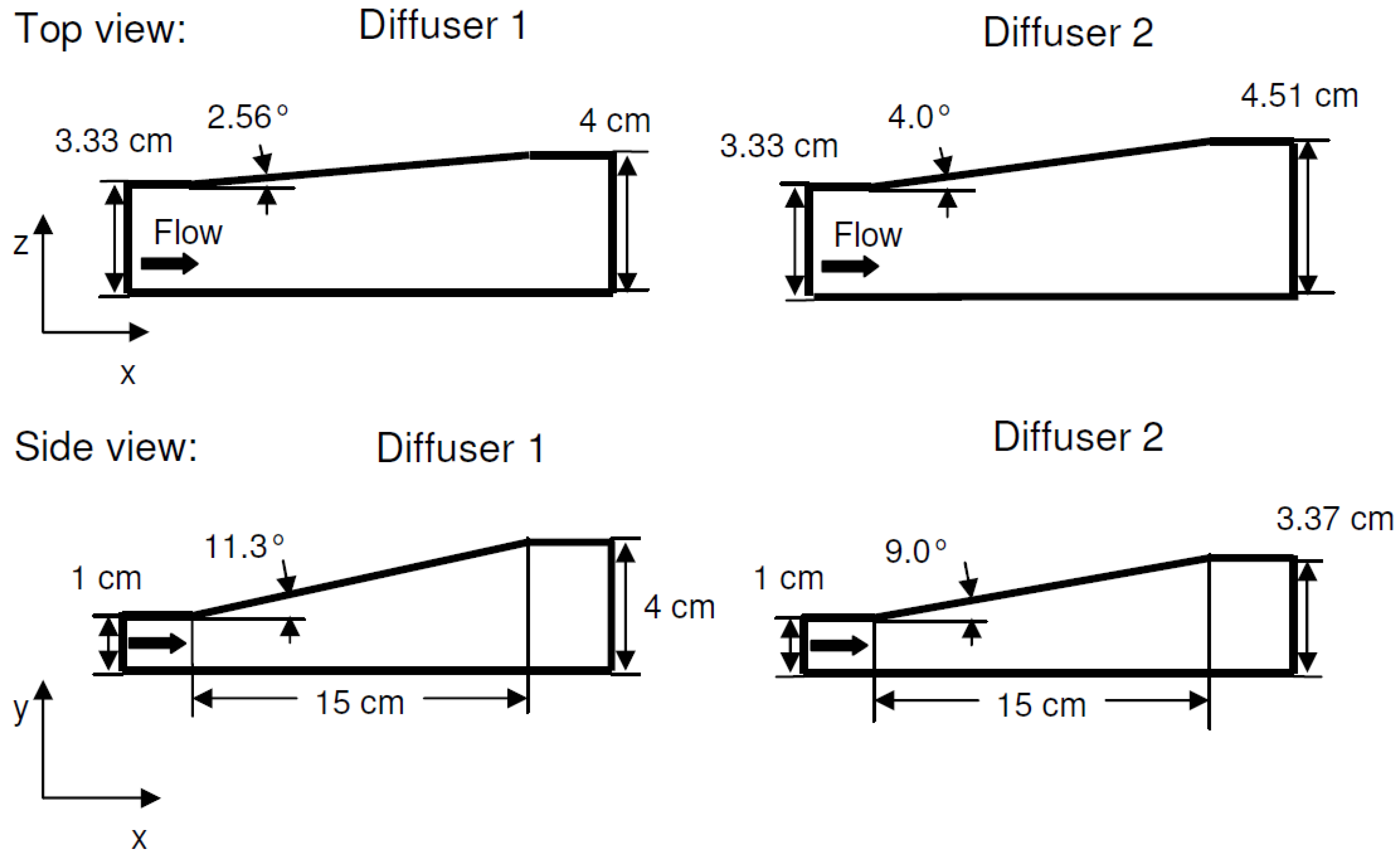
2009Cherry et al. [23]MRV (magnetic resonance velocimetry)Three-dimensional flow in a diffuser, R e τ = 320 . The geometry is asymmetric in spanwise and transverse directions.
2022Simmons et al. [24]LDV, oil-film flow visualizationThree-dimensional flow separation from a smooth ramp and sidewalls, three separation cases, R e τ = 2600 . Symmetric sidewalls may cause alternating asymmetric separation.
Following the work of Obi et al., another experiment on a plane diffuser was conducted by Buice and Eaton [21,25]. Their objective was to improve the set-up of Obi et al.’s experiment by minimizing the effects of end-wall separation. To achieve this, they used splitter plates that started 6 H upstream of the beginning of the diffuser, and boundary layer suction was employed through drilled holes within the first 5 H of the splitter plates. Additionally, they chose a wider and longer domain, with an inlet aspect ratio of 40 (ref. [19] used a value of 35) and an outlet channel length of 56 (ref. [19] used a value of 40). Their diffuser set-up and a scheme of the separation are shown in Figure 3 and Figure 4, respectively. The inlet channel flow was stated to be fully developed and spanwise homogenous over 85% of the channel width in tests without the diffuser section. However, in the complete set-up, integrating the upstream and downstream velocity profiles of the diffuser showed a large discrepancy in the mass flow rates, indicating that some secondary flow effects remained.
Another successor to Obi et al.’s experiment was a study by Törnblom et al. [22,26] on a plane diffuser with an opening angle of 8.5° and a higher Reynolds number of R e τ 980 . The change of the opening angle from 10° to 8.5° was made in order to reduce the unsteadiness of the separation and reattachment points by reducing the size of the separation zone. To ensure two-dimensionality in the mean flow, a high aspect ratio (50:1) and end-wall boundary layer suction were used. Velocity profiles and Reynolds stresses were measured by employing the Particle Image Velocimetry (PIV) technique. It is stated that a smaller separation bubble size might indicate this case to be more complex for turbulence modeling.
These plane diffuser experiments have been used as validation cases in many computational studies and are attractive for several reasons. Firstly, the fully developed channel inlet flow is relatively easy to replicate in simulations because it is unambiguous. Secondly, two-dimensional flows are often desirable because they are more computationally affordable compared to three-dimensional flows, especially for methods like LES and grid convergence studies. Finally, the measurements are well-documented, and some of the data are open access (such as [21] for the Buice and Eaton case).

2.2. Three-Dimensional Separated Diffuser

Fully three-dimensional diffuser experimental data were obtained by Cherry et al. [23,27] for two slightly different configurations. The geometry in this study featured a diverging bottom and sidewall (Figure 5), with any symmetries being intentionally avoided. The inlet flow is a fully developed flow in a square channel at a Reynolds number R e τ of approximately 320 (which corresponds to R e = U b 2 δ / ν 10,000 , where U b is the bulk velocity). Three grids were included at the upstream end of the development channel section to achieve greater flow uniformity. The goal of this experiment was to provide mean velocity data and static pressure measurements for a three-dimensional diffuser and investigate the sensitivity of the separation to relatively small changes in the geometry. The outlet transition sections consisted of a 10 cm constant cross-section channel and then a 10 cm contraction into a circular outlet 1 in diameter.
The mean velocity components were measured by using magnetic resonance velocimetry (MRV), and the resulting velocity contours were presented in their work [23]. It was stated that while, in both diffusers, the flow separated at a sharp corner of the geometry, the overall separation regions were vastly different. In Diffuser 1, the separation region was found to be nearly two-dimensional, while in Diffuser 2, it was three-dimensional for the entire length of the diffuser. Therefore, it was concluded that the flow exhibits a high degree of sensitivity to the geometry, making it challenging to accurately capture via CFD.

2.3. Three-Dimensional Flow over a Smooth Backward-Facing Ramp

A more recent validation test case comes in the form of an experiment of the flow over a smooth backward-facing ramp by Simmons et al. [24,28]. The ramp geometry in this test was two-dimensional, and the three-dimensionality was caused by the effect of sidewall separation on the core flow, with the aspect ratio being intentionally low. The test section geometry is given in Figure 6. The inlet flow in this test case was a zero pressure gradient flat plate turbulent boundary layer flow at Mach number M = 0.2 and R e τ 2600 (which corresponds to R e h = U h / ν 8.27 10 5 , with h being the ramp height). The flat plate boundary layer was tripped by a 4 in wide strip of distributed sand grain roughness with an average roughness element size of 2 10 4 m located on bottom and sidewalls 1.2 m upstream of the ramp leading edge. The experimental set-up featured a flexible top-wall contour, allowing for the adverse pressure gradient to be adjusted. The ramp geometry was constructed with zero first- and second-derivative end conditions. The width of the domain was approximately 4.55   h, allowing the mean inlet flow to be two-dimensional up until the start of the ramp.
In this experiment, LDV was used to measure velocity profiles and Reynolds stresses on the bottom and sidewalls. Additionally, surface skin friction lines were obtained by the oil-film visualization technique. The measurements are presented for three top-wall configurations and describe a large separation case, a small separation case, and an attached flow case. This validation case certainly poses many difficulties for turbulence modeling, such as the computational cost needed to resolve all of the boundary layers. This and other challenges will be discussed further in Section 3 and Section 4.

3. Overview of Computational Studies

This section will focus on a selective list of attempts of numerical modeling the experiments described in the previous section. A summary of the computational works can be found in Table 2. As seen from Table, RANS simulations can fall short of accurately predicting three-dimensional flows or flows with a smaller separation bubble. A more thorough discussion is presented further on in this paper.

3.1. Plane Asymmetric Diffuser Simulations

Most computational studies featuring plane asymmetric diffusers use an opening angle of 10°, as was the case in Buice and Eaton’s study [21]. The steady RANS simulations are typically two-dimensional, while the scale-resolving simulations are periodic in the spanwise direction. The simulations are usually split into two parts. Firstly, the inlet flow is obtained in a separate periodic channel flow simulation. This step is not complicated as there are data from both the experimental and DNS studies available at the simulated Reynolds number. The inlet flow is then used as a boundary condition for a diffuser simulation. One may instead opt for using the experimental set-up and simulate the long section of developing channel flow along with the diffuser, as was the case in the work of DalBello et al. [29].
Unsteady numerical data on the 10° diffuser test case can be found in the wall-resolved LES study of Kaltenbach et al. [30]. They used an incompressible three-dimensional code based on a hybridized second-order finite difference/spectral approach. A Fourier collocation was used in the spanwise direction, and a second-order finite difference approximation was employed in the other directions. Time stepping was conducted through a semi-implicit scheme in which the viscous terms were integrated with the Crank–Nicolson method, and the other terms were integrated with a low-storage third order Runge–Kutta scheme. They used a dynamic Smagorinsky subgrid-scale model in which the dynamic model coefficient was calculated using the least-square approach [31]. They performed a grid convergence study and investigated the influence of the spanwise domain size. It was found that changing the domain width from four channel heights to two has little effect on the mean channel flow but affects the diffuser part of the domain, where the turbulence length scales are much larger. With a narrower domain, the flow is found to reattach more slowly. The limitation of the spanwise length scale of the flow can be seen in Figure 7. Good agreement with the experimental data was obtained for the mean flow overall, but r.m.s. values of velocity fluctuations had deviations outside of the measurement error bounds. Another LES study for this test case was performed by Wu et al. [32]. They used a finite volume code with an unstructured fractional step method and an implicit second-order Crank–Nicolson scheme for all of the terms. The diffuser domain width was chosen to be four channel heights (in accordance with a study by Kaltenbach et al.), and a dynamic Smagorinsky model was used. They mainly investigated the attached internal layer flow close to the flat wall of the diffuser.
A numerical approach similar to the one in [30] was used to perform wall-resolved LES simulations for a diffuser with a smaller opening angle [22] in a study by Herbst et al. [33]. They investigated the dependence of the separation bubble size on the inflow Reynolds number and validated their method by including a simulation of the Buice and Eaton diffuser. The overall trend observed in the study was an increase in the separation bubble size at higher Reynolds numbers, which agrees with Obi et al.’s experimental study [19]. The authors reported a small separated region appearing at the flat diffuser wall at lowest of the studied Reynolds numbers. A comparison of skin friction distributions along both diffuser walls at different Reynolds numbers can be found in Figure 8.
Table 2. Selective list of attempts at modeling the asymmetric diffuser experiments.
Simulated
Experiment
YearAuthorMethod and Details
Obi et al. [19]2006Wu et al. [32]LES
Main focus is on the internal layer flow on the flat diffuser wall.
1993Obi et al. [19] RANS   ( k - ε and DRSM)
More advanced second-moment closures are needed. Both simulations deviated from the experimental data.
1999Apsley, Leschziner [34] RANS   ( various )
Linear and non-linear eddy viscosity models are investigated. Non-linear models were sensitive to modifications in the ε-equation.
Buice and Eaton [21]1999Kaltenbach et al. [30]LES
Reattachment is delayed due to a narrow spanwise domain. Velocity fluctuations deviate by up to 20%.
2005Davidson, Dahlström [35]Hybrid RANS/LES
Log-Layer mismatch in channel flow simulation, improved by forcing. Separation bubble size in the diffuser simulation is overpredicted.
2005DalBello et al. [29]RANS (various turbulence models)
Several turbulence models were tested. Grid sensitivity study was performed for the SST model with the use of wall functions. All models showed early separation.
Törnblom et al. [22]2007Herbst et al. [33]LES
Three   test   cases   with   R e τ 260 ,   480   and   980 .  
Separation   bubble   size   increases   at   higher   R e τ .
2007Törnblom, Johansson [36]RANS (DRSM)
Underpredicted separation bubble size. The main focus of the study is separation control.
2004Gullman-Strand et al. [37]RANS (EARSM)
Underpredicted separation bubble size. The Buice and Eaton diffuser [21] was also simulated in this study.
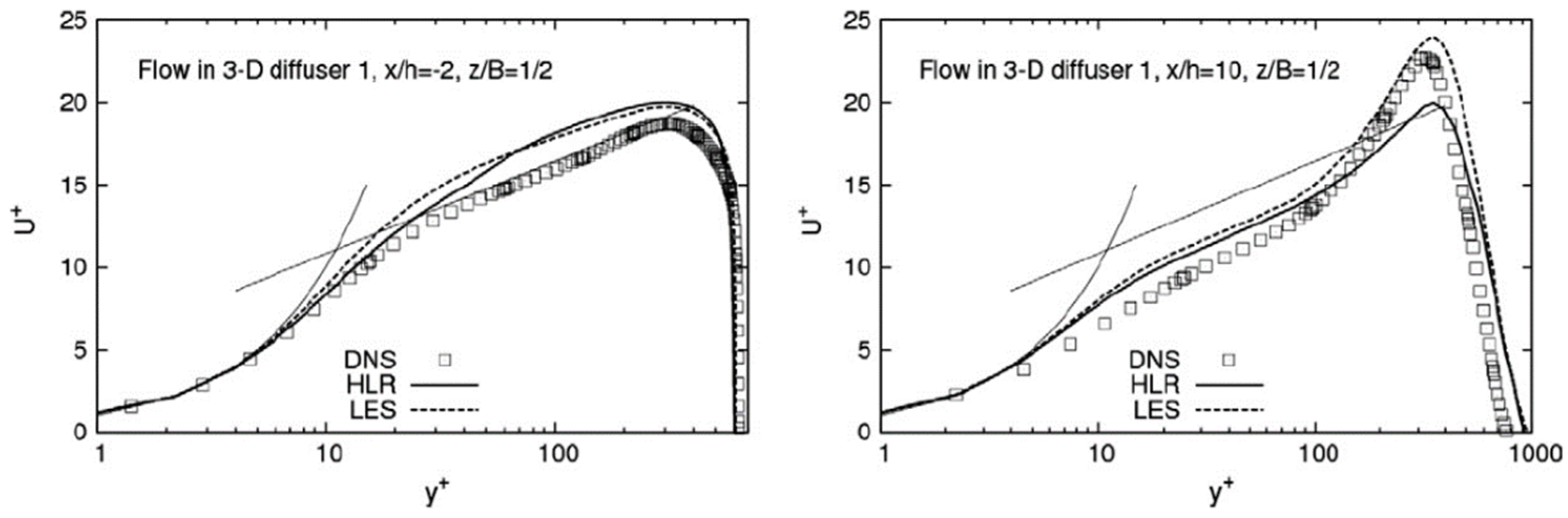
Cherry et al. [23]2011Ohlsson et al. [38]DNS
Close agreement with the experimental data.
2010Jakirlić et al. [39]LES, Hybrid RANS/LES
Reasonable results obtained with both methods.
2009Von Terzi et al. [40] LES ,   RANS   ( k - ω )
RANS fails to accurately predict velocity profiles and the separation. LES shows reasonable agreement with the experiment.
2010Abe, Ohtsuka [41]Hybrid RANS/LES
Results are in line with [39].
Simmons et al. [24]2022Rizzetta, Garmann [42]LES
Two   cases   with   R e τ 450   and   R e τ 1300 .
Results were affected by a narrow domain.
2022LES Workshop on Smooth-Body Separation 2022 [43]LES, Hybrid RANS/LES
Simulations were spanwise periodic. Several
simulation difficulties are addressed.
A small separated region appeared at the flat diffuser wall at the lowest Reynolds numbers. A comparison of skin friction distributions along both diffuser walls at different Reynolds numbers can be found in Figure 7 and Figure 8.
The RANS turbulence model performance for the Buice and Eaton diffuser was investigated by DalBello et al. [29]. Their simulations were conducted with a three-dimensional RANS solver [44] using a node-centered finite volume approach. Local time stepping and a second-order Roe upwind scheme with a stretched grid modification were employed. They used k - ε [45], Menter SST [46] and Spalart–Allmaras (SA [47]) turbulence models, and an Explicit Algebraic Reynolds Stress (EARSM [48,49]) turbulence model to simulate the diffuser flow and compared the resulting velocity profiles and skin friction distributions to those measured in the experimental study. The EARSM and SST models showed the closest resemblance to the data. Out of all the eddy viscosity models studied, k -ε was the least accurate at predicting both the separation and the reattachment points (both too early). The SST and SA models were found to predict early separation and overestimate the separation bubble size by about 24 % . The EARSM model showed the closest predictions overall, and it was stated that the computational time for this model was not significantly more expensive than it was for the linear eddy viscosity models. A comparison of separation streamlines for all the turbulence model tests can be found in Figure 9. Another rather thorough overview of turbulence model performance (linear and non-linear eddy viscosity models) can be found in [34], in which the authors notice that although the more advanced turbulence models have a more justified basis, they may perform only marginally better than simpler eddy viscosity models. Their superiority becomes more questionable as the complexity of the flow configuration increases (at least, this seems to be the case at the time of writing).
A RANS simulation with the EARSM model [52] was performed for a diffuser with both 10° and 8.5° opening angles by Gullman-Strand et al. [37]. In this work, a finite element code generated with the femLego toolbox [53] was used with piecewise linear elements and a fractional time step method. They report qualitative agreement between the mean velocity profiles, skin friction, and pressure coefficients obtained in their simulation for both cases and the experimental data. The quantitative differences, including the reduced backflow strength, were stated to be caused by model imperfections. For the 10° case, although the flow separates and attaches slightly earlier than in the experiment, overall, the separation bubble size and height are rather accurate. The 8.5° case appears to be more difficult to accurately capture since the separated region is smaller. For this case, the model predicted early reattachment of the flow and a much thinner separation bubble size than in the experimental data, as seen in Figure 10. A variant of a Differential Reynolds Stress Model [36] showed somewhat similar behavior to the EARSM simulation [37]. The size of the separation bubble was underpredicted, and an unphysical shape near the reattachment region was observed (Figure 11). Such an anomaly in this region was noted by several other authors [19,54,55] who used DRSM turbulence models. This was explained by the excessive values of the integral length scale produced by DRSMs near the reattachment point. The known corrections to this issue [55,56] are based on the idea of reducing the turbulence length scale L = k 3 / 2 / ε in these regions, as outlined by Yap [57].
The performance of the RANS/LES hybrid method was investigated by Davidson and Dahlström [35]. They used an incompressible flow simulation with a code using a second-order central difference spatial scheme, an implicit two-step time-advancement approach including a Crank–Nicolson scheme, and a multigrid method [58] for the Poisson equation. The RANS/LES interface was set to 10 cells away from the walls at the inlet. Downstream from the inlet, it was computed by requiring the conservation of the volume flow rate in the URANS region throughout the diffuser (instantaneous interface location can be seen in Figure 12). A differential equation for turbulence kinetic energy k was solved in both regions, and the turbulent viscosity was defined algebraically as a function of k and a turbulence length scale. Instantaneous inlet boundary conditions were prescribed using the data from a developed channel flow DNS simulation. With the RANS/LES interface located in such a way, most of the separated region was simulated in URANS regime. Nevertheless, the reported velocity profiles showed good agreement with the experimental data. To resolve the separated regions in LES regime, the authors of [35] performed another simulation wherein the RANS/LES interface was moved close to the bottom wall (10 cells away from it throughout the diffuser). In that simulation, the reported results showed much worse resemblance to the experimental data. The somewhat surprising results from this simulation can be explained by the use of coarse meshes (as noted by the authors), which were insufficient for LES to properly resolve the relevant scales of the separated flow. In this work, a commonly observed unphysical shift in the mean streamwise velocity profile [59] was spotted in a hybrid method channel flow simulation. This shift is attributable to the poor boundary conditions provided by the URANS region to the LES region. In order to alleviate this issue, artificial sources of velocity fluctuations were added to the momentum equations at the RANS/LES interface. The fluctuations were generated from the channel flow DNS data and eliminated the problem. The same method was used for the diffuser simulation; however, no improvement was obtained there.
Let us summarize this series of plane asymmetric diffuser simulations. Despite the simplicity of the geometry, accurate prediction of the occurring separation and its dependence on slight geometry changes is not a trivial task. While large eddy simulations seem to be successful at reproducing the experimental results, solving Reynolds-averaged Navier–Stokes equations often fails to do the same. One may hope that the commonly used one- or two-equation turbulence models will be accurate enough to use for more complex separated flows, although some models perform slightly better than the others. Reynolds stress models may be promising if one wishes to keep the computational cost lower than what is needed for eddy-resolving methods. Note that the models used in the studies above are a bit outdated. It is recommended to use more advanced models that have proven their ability to deal with some of the past issues, e.g., the streamline back-bending near the reattachment points. The use of recently developed corrections to DRSMs specifically aimed at improving the prediction of separated flows [60,61] may be beneficial. Hybrid RANS/LES methods may offer further improvement over RANS solutions; however, they do have stricter grid and time step requirements.

3.2. Three-Dimensional Separated Diffuser Simulations

The three-dimensional diffuser experiment offers further numerical challenge in predicting the separation and testing model sensitivity to slight changes in diffuser expansion angles. In addition to the experimental measurements, data from a DNS [38] and several LES simulations [39,40] are available for model validation.
The inability of the RANS approach to predict such complex separated flows was shown in the works of Von Terzi et al. [40] and Cherry et al. [23]. In [40], they performed an incompressible flow simulation using a finite volume solver [62] with a second-order accuracy spatial approximation (central difference scheme for viscous fluxes and an upwind scheme for convective fluxes) and a second-order implicit multi-step method for time advancement; mass conservation was achieved by the SIMPLE algorithm, with the pressure–correction equation being solved by the strongly implicit procedure (SIP) of Stone. They applied the standard Wilcox k - ω [63] turbulence model and tested two different inlet conditions: uniform inlet velocity profile (simulation Ia) and fully developed channel flow profile (simulation Ib). A comparison of velocity contours between RANS and an LES simulation IIa at one cross-section within the diffuser is shown in Figure 13. The LES solution was in reasonable agreement with the experimental results, while both of the RANS simulations failed to correctly predict separation bubble size and location. A comparison of velocity profiles at several streamwise locations (not shown here) also proved that RANS was unsatisfactory for this flow. In the work of Cherry et al. [23], RANS results obtained with the Fluent solver (second-order symmetric discretization in time and space) and the SST turbulence model are reported (with other eddy-viscosity models stated to bring comparable results). They reported that, in RANS simulations, the flow separates from a sidewall instead of on the top wall, and the separation happens earlier than was shown in the experiment. The failure at predicting separation in one of the 3D diffusers renders this method inadequate for investigating the effects of slight geometrical changes.
One of the eddy-resolving simulations for this test case was provided by Von Terzi et al. [40]. For these simulations, they used the same solver as for the RANS described above. A second-order central difference scheme was employed for the viscous and convective fluxes, and an explicit three-step low storage Runge–Kutta method was used for time stepping. They performed an LES for both of the diffusers featured in the experiment with a standard Smagorinsky subgrid-scale model and van Driest damping near walls. They used an adaptive wall function [62] approach, in which the wall functions are deactivated in well-resolved regions and near separation and reattachment points. Grid convergence and the influence of inlet and outlet buffer regions was investigated. This work was the first to feature an LES for both of the diffusers used in the experiment. The difference in the shapes of the separated regions obtained in the simulations is shown in Figure 14. The small separated regions (labeled SB1) are artifacts of the numerical set-up that are stated to have no effect on the downstream results. The separation bubble of Diffuser 1 becoming close to two-dimensional was in accordance with the experimental data, as was the separation point being in one geometrically triggered spot. The LES simulation succeeded in displaying the effect of slight expansion angle changes. The results of mean streamwise velocity profiles and the fraction of separated cross-sectional area were reported to be within measurement uncertainty and therefore considered to be in acceptable agreement with the experimental data. Additional buffer regions at the inlet and outlet had a negligible influence on the results.
Another eddy-resolving study of the 3D diffuser was featured in the work of Jakirlić et al. [39], with the chosen geometry being Diffuser 1. They used a finite volume code [64] for incompressible flow simulation with a SIMPLE based algorithm for pressure correction. The Crank–Nicolson scheme was employed for time discretization, and a second-order central difference scheme was used for special discretization in both the LES and hybrid simulation with a mix of an upwind scheme for the k and ε equations. They performed an LES simulation with the dynamic Smagorinsky subgrid-scale model and a hybrid RANS/LES simulation that combined a near-wall k - ε RANS turbulence model with the standard Smagorinsky subgrid-scale model. The hybrid RANS/LES method used in this study was zonal; the interface was defined through a flow-dependent algorithm and located at dimensionless distances y + , z + 50 from the walls. A simultaneously running periodic developed channel flow simulation provided inlet boundary conditions for the diffuser. It was noted that the periodic channel may have been too short and that the periodic boundary condition for it may have introduced unphysical spatial periodicity into the flow [65]; however, this set-up was chosen in order to lower the total computational cost of the simulations.
The velocity profile (Figure 15) obtained in the hybrid simulation exhibited a shift near the RANS/LES interface location ( y + 50 ) , similar to the one observed by Davidson and Dahlström [35], as was discussed above. Forcing or other methods were not used in this simulation in order to alleviate the velocity shift, as the authors state the slight bump in the inlet velocity profile did not significantly affect the flow downstream. While, in the current simulation, that may be true, in general cases, an incorrect inlet velocity profile may affect the separated region downstream more strongly. A comparison of axial velocity isocontours at several streamwise locations for both simulation methods is illustrated in Figure 16. The separation bubbles are in qualitative agreement with the experimental results for the LES and hybrid RANS/LES simulations. A difference between the methods can be seen at the location x / H = 5 ; LES is more accurate there as it produces a symmetrical separation bubble in the upper right corner, which is correct according to the experiment. Hybrid RANS/LES produces an asymmetric separation bubble at this location; however, the difference diminishes closer to the end of the diffuser.
A hybrid RANS/LES study of Diffuser 1 with a more advanced turbulence model was conducted by the authors of [41]. They used a finite volume code [66] with a SIMPLE solution scheme and a Crank–Nicolson time integration method. A second-order central difference scheme was used for each term, except the convection terms in the k and ε equations of the hybrid simulation and the RANS simulation, for which a TVD scheme was employed. They used a non-linear eddy viscosity model [67] in the RANS region and a subgrid-scale model [68] in the LES region of their simulation. Separate RANS and LES simulations with these models were performed on the same grid that was used for hybrid RANS/LES. The results showed that, despite being more advanced, the RANS model behaves similarly to the Wilcox k - ω model, with the separation occurring mostly on one side of the diffuser (as in Figure 13). Due to it being used on a grid too coarse near the wall, the LES simulation was also shown to give inaccurate results, although the separation bubble on the upper wall was predicted better than in the RANS simulation and close to being two-dimensional at the end of the expanding part. The shape of the separated regions the hybrid RANS/LES simulation was in better agreement with the experimental data, looking similar to the hybrid simulation in Figure 16. The authors suggest that the hybrid simulation results may be improved by using a simultaneous channel flow simulation as the inlet boundary condition instead of the precursor simulation used in their work. Perhaps finer grids could also be beneficial since, with their base grid, the RANS/LES interface seems to take up a substantial part of the boundary layers (Figure 17).
Regarding the results of the computational studies described above, we can draw the following conclusions. Firstly, RANS is not a reliable tool for predicting complex three-dimensional separated flows, even with more advanced turbulence models. Secondly, since LES simulations of such flows are generally much too expensive, a properly conducted hybrid RANS/LES may be a reasonable alternative to keep the computational cost lower while simultaneously allowing for the separated regions to be properly resolved. Hybrid methods are still in a state of constant improvement, and some of them are more forgiving of coarse grids than others. Techniques like Partially Averaged Navier–Stokes (PANS [69]) or the more recently established Active-Model Split [70] may contribute to making hybrid simulations more affordable for engineering purposes.

3.3. Simulations of the Three-Dimensional Flow over a Smooth Backward-Facing Ramp

The final set of computational studies in this section is dedicated to the experiment that was conducted and recently published by the authors of [24]. This test featured a separated flow over a smooth backward-facing ramp, and while the ramp itself was two-dimensional, the resulting separation was three-dimensional due to the influence of symmetrical sidewalls. Since there are not a lot of numerical studies available in the literature; we will focus on the LES study reported by Rizzetta et al. [42] and a workshop on smooth-body separation [43], both of which provide valuable insight despite the choice of a spanwise-periodic set-up. Further simplification can be achieved through the use of a flat horizontal top wall with an inviscid boundary condition.
We will start with discussing the wall-resolved LES study [42], which provided reference data for the workshop [43]. They used an implicit approximately factored finite difference algorithm [71] that employed Newton-like subterations [72]. The spatial derivatives were approximated with a second-order central difference scheme, and the non-linear artificial dissipation [73] was added to improve stability. For temporal approximation, a second-order-accurate backward-implicit scheme was used with three subiterations per timestep. A relatively high Reynolds number was used in the experiment ( R e = 7.0 × 10 6 based on freestream quantities and the ramp length). Thus, the simulation was conducted in a simplified set-up resembling an earlier backward-facing ramp LES [74,75] performed at a much lower Reynolds number. In order to make the comparison of the results more affordable for the workshop participants, LES simulations were performed at two lower Reynolds numbers ( 1.0 × 10 6 and 3.0 × 10 5 ). The numerical technique used in this study was the Implicit LES approach [76,77], meaning that the filtered Navier–Stokes equations could be solved without an explicit subgrid-scale model. The inlet boundary condition for the ramp simulation was a classic flat plate boundary layer that matched the experimental boundary layer thickness δ . Such boundary conditions are more ambiguous than a fully developed channel flow and demand a separate flat plate simulation. Once the target boundary layer was obtained, the ramp mesh was appended downstream of that location. The number of grid points necessary to perform a thorough resolution study was, of course, extreme (up to 800 million and 1.5 billion grid points for the finest flat plate and ramp meshes, respectively).
It was found that, for the lower Reynolds number, the ramp affected the boundary layer at the inlet, making it 19 % thinner than in the experiment. For the higher Reynolds number, this was not the case. The grid convergence study showed that the coarsest mesh failed to accurately predict the skin friction distribution, and as the mesh was refined, the solution slowly approached a grid-independent state. From our point of view, this is a warning sign that more attention should be paid to the underlying physical model used in these simulations. The subgrid-scale model (or the numerical method which substitutes it) may play a more important role than just a dissipation of kinetic energy, especially in near-wall and separated flows; for instance, the replication of the backscatter event might improve the simulation results [78]. If this proves to be true, a differential model for the individual components of a subgrid-stress tensor could be a remedy in such simulations [79].
The authors of [42] also suggested that the solution could be improved by resolving a longer downstream domain (longer than two ramp lengths). Even more importantly, it was reported that a domain width of 4 δ i n is not sufficient to accurately capture the downstream part of the domain (whereas it was sufficient for the flat plate). This suggests that even more computational resources are needed to accurately simulate this flow. Nevertheless, the results of this study provided valuable data for CFD modeling and were used for comparison by the workshop participants (with the same domain width imposed). Mean and instantaneous streamwise velocity contours for the two Reynolds numbers used in this study are shown in Figure 18. The separation point for both cases is reportedly almost the same, and the attachment point is slightly further for the higher Reynolds number. Velocity, turbulent kinetic energy, and turbulent shear stress profiles are provided in this study, along with the skin friction distribution and the turbulence kinetic energy spectra.
The smooth body separation workshop was focused mainly on LES used in conjunction with wall models (WMLES). Eleven scientific groups who used various numerical methods and subgrid-scale models participated in this workshop. According to the authors of [80], only one of the groups performed not WMLES but hybrid RANS/LES simulations using the SST-IDDES approach [81]. They implemented the same simplifications to the experimental set-up as in the reference LES described above and simulated the case R e = 1.0 × 10 6 . While these are preliminary results, they still provide useful information for those who wish to simulate the experimental set-up as it is or its simplified version. Figure 19 presents the separation and reattachment points obtained by different groups on the finest meshes. It is apparent that correctly predicting the reattachment location posed a lot of difficulties, while the separation location for most of the participants was rather close to that obtained in the reference LES simulation. A more discouraging outcome from the workshop was the difficulty experienced in obtaining a grid-converged solution. The separation bubble size tends to increase with grid refinement; however, it was stated that none of the groups succeeded at this, even at grids with over 100 million cells. The SST-IDDES simulation present in the workshop results obtained questionable results, with the shape of the separation region being unphysical; therefore, it cannot yet be used for comparison. The cause of this poor result still needs to be investigated. It is known that SST-IDDES in itself can perform relatively well for such a flow [81].
Other set-up details that were studied in this workshop included investigating the influence of inflow and outflow locations and the domain width influence. It was shown that the outflow boundary does not influence the solution upstream if set further than four ramp lengths away from the beginning of the ramp. It was demonstrated (Figure 20) that the results are highly sensitive to the domain width, with the width of 40 δ i n still not being quite enough (a value of 4 was used in the reference LES and by most of the workshop participants). An increase in the separation bubble size with the use of a too-narrow domain is in accordance with the reference LES results for a diffuser flow discussed in [30].
As can be seen from the computational results, this test case poses a challenge from both physical and numerical points of view. Physical issues include the insufficiently studied role of the subgrid-scale model. It looks like some physical mechanism is not replicated in the simulations, which results in slow grid convergence. The main numerical issue is the computational cost of the simulations associated with the required grids (typically, 10 8 to 10 9 grid points, even in a simplified set-up). If one decided to simulate the experimental set-up without simplifying it, more difficulties arise. An obvious problem would be the need to correctly model the boundary layers (and separation) on all of the walls along with the secondary flows in the corners of the diffuser. The latter demands a near-wall model that is able to capture such types of flow, e.g., a Reynolds stress model. Overall, hybrid RANS/LES simulations are more likely to capture the separated regions correctly. The RANS approach may overpredict the separation occurring on the sidewalls, which can lead to a smaller separated region along the curved wall. If the target inlet boundary layer is to be obtained from a full experimental geometry simulation instead of a separate flat plate one, then the flow needs to become turbulent at a correct location. In the experiment, a sand strip of a known average roughness element size is used on the bottom and side walls. If the sand strip is to be modelled, then it may take some time to tweak the roughness model for obtaining a correct inlet flow, e.g., vary roughness model constants, sand strip length, and placement. Note that this tweaking is empirical in nature [82]. Additionally, the fact that the sidewalls are symmetrical can cause additional separation unsteadiness. For this reason, in preliminary simulations, one may employ an unsteady numerical set-up instead of a steady approach.

4. Conclusions

This section summarizes the essential points of the review. A selective list of numerical studies concerning asymmetric subsonic diffusers was presented; the experimental studies that were modelled were sequenced from least to most physically and numerically complicated. Plane asymmetric diffusers with high aspect ratios that allow the separated flow to be two-dimensional are considered more basic. They allow one to test a model’s ability to properly capture the boundary layer flow and the separation occurring on a single wall and allow one to estimate the model’s sensitivity to relatively small geometry changes (different expansion angles). The two-dimensionality is very convenient for CFD as it allows to decrease the computational cost of the simulations; however, this does not make the task trivial.
The commonly used RANS approach with eddy-viscosity turbulence models often fails to produce acceptable results for separating flows. Early separation in numerical results is a frequent side effect of such simulations. Reynolds stress models are more advanced and may offer improvement in RANS simulation accuracy; therefore, it is generally recommended to use them instead if one chooses a steady framework. However, even RSMs may still struggle with accurately predicting smaller separated regions (as in the 8.5° opening angle diffuser). Eddy-resolving methods, such as LES, are capable of closely matching the experimental data in flows of varying complexity; however, this is not always considered to be an accessible approach due to the high computational cost. A more cost-effective strategy involves the use of hybrid RANS/LES methods that have been steadily improving for over 20 years. They may provide results that are not much worse than pure (wall-resolved) LES, but only if the simulation is set up properly. The method should switch to LES only when the grid resolution allows it and when there is enough unsteadiness (either synthetic or geometry-induced) for resolved eddies to evolve.
Compared to plane asymmetric diffusers, the three-dimensional diffuser outlined in Cherry et al.’s study is slightly more complex. This test case provides two geometries for testing the model sensitivity and demands a model that is capable of accurately capturing 3D separation patterns. The DNS data available for the experiment supports and supplements the measurements and provides more information for model validation. In its current state, the RANS approach was shown to be unsuitable for this geometry as the simulations exhibited a completely different separation pattern from the experimental data, predicting the separated region to be mostly on one of the sidewalls. Both LES and hybrid RANS/LES methods were demonstrated to be capable of providing satisfactory results for this flow. The overall computational cost of the simulations is not excessive due to the relatively low Reynolds number of the flow.
The final experimental set-up that considered in the current review was the recently published backward-facing ramp test case by Simmons et al. This set-up features a 2D ramp geometry and a substantial 3D separation pattern due to the close proximity of the sidewalls. One of the issues that makes this test complicated is the high computational cost due to the Reynolds number used in the experiment, even if the set-up is simplified to a spanwise-periodic one. The simulated flow being homogeneously spanwise still suggests a need for a sufficiently wide computational domain (over 40 inflow boundary layer thicknesses), which further increases the number of grid points. To simulate the experiment without simplifications, one needs a reliable near-wall model capable of describing secondary flows in the sidewall-ramp juncture and interaction of the separated boundary layers. We suggest that Reynolds stress models are promising in that regard. As wall-resolved large eddy simulations are prohibitively expensive for this test, hybrid RANS/LES methods are probably a more attainable choice, provided that the numerical set-up is reasonable. Another subtlety that may take some time to grasp is obtaining a correct inflow boundary layer profile. If the entirety of the experimental set-up is simulated, then an appropriate roughness model needs to be used to trip the flow.
An important issue to discuss from a numerical point of view is the difficulty in obtaining a grid-converged solution, which, among the tests considered was highlighted in the final one. One of the reasons for this may be that the subgrid-scale model does not replicate some physical effects (such as backscatter) that are present in the experiment. Further research into this is required. Additionally, a numerical method needs to be properly selected, both for spatial approximation and time integration. Today it is common to use hybrid central difference/upwind schemes. If a near-wall RANS model used in a simulation includes an ω -equation, then it is recommended to use the first off-wall grid point spacing equal to y + 0.1 instead of the general y + = 1 , since such models are more sensitive to this parameter. One last thing we would like to note is that, to simulate subsonic flows, one needs to ensure that appropriate boundary conditions are used. Naïve approaches may generate growing disturbances due to an imbalance between inlet and outlet boundaries. It is recommended to employ characteristic boundary conditions.

Author Contributions

Conceptualization, A.B. and V.S.; writing—original draft preparation, A.B.; writing—review and editing, A.T.; supervision, V.S. All authors have read and agreed to the published version of the manuscript.

Funding

The research was funded by a grant from the Russian Science Foundation No. 21-71-10105, https://rscf.ru/en/project/21-71-10105/ (accessed on 24 March 2023).

Data Availability Statement

No new data were created or analyzed in this study. Data sharing is not applicable to this article.

Acknowledgments

The authors are grateful to the reviewers for their valuable comments, which helped improve this review.

Conflicts of Interest

The authors declare no conflict of interest.

Nomenclature

R e Reynolds number
M Mach number
u τ friction velocity
δ channel half-height
ν kinematic viscosity
H channel height
U b bulk velocity
U freestream velocity
h ramp height
L ramp length
k turbulence kinetic energy
ε dissipation rate of turbulence kinetic energy
ω turbulence frequency
C p pressure coefficient
l z integral length scale
C f skin friction coefficient
L turbulence length scale
δ i n inlet boundary layer thickness
L z domain width
x, y, zcartesian coordinates
Subscripts and superscripts
inparameters at the model inlet
+law of the wall variables
τ friction variables
Acronyms
LESlarge eddy simulation
RANSReynolds-averaged Navier–Stokes equations
URANSunsteady RANS
PANSpartially averaged Navier–Stokes
WMLESwall-modelled LES
DNSdirect numerical simulation
DESdetached eddy simulation
DDESdelayed DES
IDDESimproved DDES
RSMReynolds stress model
EARSMexplicit algebraic RSM
DRSMdifferential RSM
LDVlaser Doppler velocimetry
PIVparticle image velocimetry
MRVmagnetic resonance velocimetry
CFDcomputational fluid dynamics
r.m.s.root mean square
SSTshear stress transport
SASpalart–Allmaras

References

  1. Venturi, G.B. Recherches Expérimentales sur le Principe de la Communication Latérale du Mouvement Dans Les Fluides, Appliqué à L’explication de Différents Phénomènes Hydrauliques; Houel et Ducros and Théophile Barrois: Paris, France, 1797. (in French) [Google Scholar]
  2. Patterson, G. Modern diffuser design: The efficient transformation of kinetic energy to pressure. Aircr. Eng. Aerosp. Technol. 1938, 10, 267–273. [Google Scholar] [CrossRef]
  3. Cockrell, D.; Markland, E. A Review of Incompressible Diffuser Flow: A Reappraisal of an Article by G. N. Patterson entitled ‘Modern Diffuser Design’ which was published in this journal twenty-five years ago. Aircr. Eng. Aerosp. Technol. 1963, 35, 286–292. [Google Scholar] [CrossRef]
  4. Azad, R.S. Turbulent flow in a conical diffuser: A review. Exp. Therm. Fluid Sci. 1996, 13, 318–337. [Google Scholar] [CrossRef]
  5. Simpson, R.L. A review of some phenomena in turbulent flow separation. J. Eng. Gas Turbines Power. 1981, 135, 062001. [Google Scholar] [CrossRef]
  6. Ashjaee, J.; Johnston, J.P. Straight-Walled, Two-Dimensional Diffusers—Transitory Stall and Peak Pressure Recovery. J. Fluids Eng. 1980, 102, 275–282. [Google Scholar] [CrossRef]
  7. Spalart, P. Strategies for turbulence modelling and simulations. Int. J. Heat Fluid Flow 2000, 21, 252–263. [Google Scholar] [CrossRef]
  8. Piomelli, U.; Balaras, E. Wall-layer models for large-eddy simulations. Annu. Rev. Fluid Mech. 2002, 34, 349–374. [Google Scholar] [CrossRef] [Green Version]
  9. Guseva, E.K.; Garbaruk, A.V.; Strelets, M.K. An automatic hybrid numerical scheme for global RANS-LES approaches. J. Phys. Conf. Ser. 2017, 929, 012099. [Google Scholar] [CrossRef] [Green Version]
  10. Bakhne, S.; Sabelnikov, V. A Method for Choosing the Spatial and Temporal Approximations for the LES Approach. Fluids 2022, 7, 376. [Google Scholar] [CrossRef]
  11. Eça, L.; Pereira, F.S.; Vaz, G. Viscous flow simulations at high Reynolds numbers without wall functions: Is y+≃1 enough for the near-wall cells? Comput. Fluids 2018, 170, 157–175. [Google Scholar] [CrossRef]
  12. Eça, L.; Hoekstra, M. On the Grid Sensitivity of the Wall Boundary Condition of the k-ω Turbulence Model. J. Fluids Eng. 2004, 126, 900–910. [Google Scholar] [CrossRef]
  13. Majumdar, B.; Mohan, R.; Singh, S.N.; Agrawal, D.P. Experimental Study of Flow in a High Aspect Ratio 90 Deg Curved Diffuser. J. Fluids Eng. 1998, 120, 83–89. [Google Scholar] [CrossRef]
  14. van Lier, L.; Dequand, S.; Hirschberg, A.; Gorter, J. Aeroacoustics of diffusers: An experimental study of typical industrial diffusers at Reynolds numbers of O(105). J. Acoust. Soc. Am. 2001, 109, 108–115. [Google Scholar] [CrossRef]
  15. Sullerey, R.K.; Mishra, S.; Pradeep, A.M. Application of Boundary Layer Fences and Vortex Generators in Improving Performance of S-Duct Diffusers. J. Fluids Eng. 2002, 124, 136–142. [Google Scholar] [CrossRef]
  16. Abdellatif, O. Experimental study of turbulent flow characteristics inside a rectangular S-shaped diffusing duct. In Proceedings of the 44th AIAA Aerospace Sciences Meeting and Exhibit, Reno, Nevada, 9–12 January 2006; p. 1501. [Google Scholar] [CrossRef]
  17. Delot, A.L.; Garnier, E.; Pagan, D. Flow control in a high-offset subsonic air intake. In Proceedings of the 47th AIAA/ASME/SAE/ASEE Joint Propulsion Conference & Exhibit, San Diego, CA, USA, 31 July–3 August 2011; p. 5569. [Google Scholar] [CrossRef]
  18. Mansour, M.; Kováts, P.; Wunderlich, B.; Thévenin, D.; Agrawal, D.P. Experimental investigations of a two-phase gas/liquid flow in a diverging horizontal channel. Exp. Therm. Fluid Sci. 2017, 93, 210–217. [Google Scholar] [CrossRef]
  19. Obi, S.; Aoki, K.; Masuda, S. Experimental and computational study of turbulent separating flow in an asymmetric plane diffuser. In Proceedings of the Ninth Symposium on Turbulent Shear Flows, Kyoto, Japan, 16–18 August 1993; Volume 305, pp. 305–312. [Google Scholar]
  20. Obi, S.; Nikaido, H.; Masuda, S. Reynolds number effect on the turbulent separating flow in an asymmetric plane diffuser. In Proceedings of the ASME/JSMR Fluids Engineering Division Summer Meeting 1999, San Francisco, CA, USA, 18–23 July 1999. [Google Scholar]
  21. Buice, C.U.; Eaton, J.K. Experimental Investigation of Flow through an Asymmetric Plane Diffuser; CTR Annual Research Briefs: Moffett Field, CA, USA, 1995; pp. 243–248. [Google Scholar]
  22. Törnblom, O.; Lindgren, B.; Johansson, A.V. The separating flow in a plane asymmetric diffuser with 8.5° opening angle: Mean flow and turbulence statistics, temporal behaviour and flow structures. J. Fluid Mech. 2009, 636, 337–370. [Google Scholar] [CrossRef]
  23. Cherry, E.M.; Elkins, C.J.; Eaton, J.K. Geometric sensitivity of three-dimensional separated flows. Int. J. Heat Fluid Flow 2008, 29, 803–811. [Google Scholar] [CrossRef]
  24. Simmons, D.; Thomas, F.; Corke, T.; Hussain, F. Experimental characterization of smooth body flow separation topography and topology on a two-dimensional geometry of finite span. J. Fluid Mech. 2022, 944, A42. [Google Scholar] [CrossRef]
  25. Buice, C.U.; Eaton, J.K. Experimental investigation of flow through an asymmetric plane diffuser. J. Fluids Eng. 2000, 122, 433–435. [Google Scholar] [CrossRef] [Green Version]
  26. Törnblom, O. Experimental and Computational Studies of Turbulent Separating Internal Flows. Ph.D. Thesis, KTH Royal Institute of Technology, Stockholm, Sweden, 2006. [Google Scholar]
  27. Cherry, E.M.; Elkins, C.J.; Eaton, J.K. Pressure measurements in a three-dimensional separated diffuser. Int. J. Heat Fluid Flow 2009, 30, 1–2. [Google Scholar] [CrossRef]
  28. Simmons, D.J. An Experimental Investigation of Smooth-Body Flow Separation. Ph.D. Thesis, University of Notre Dame, Notre Dame, IN, USA, 2020. [Google Scholar]
  29. DalBello, T.; Dippold III, V.; Georgiadis, N.J. Computational Study of Separating Flow in a Planar Subsonic Diffuser; No. NASA/TM-2005-213894; Glenn Research Center: Cleveland, OH, USA, 2005. [Google Scholar]
  30. Kaltenbach, H.-J.; Fatica, M.; Mittal, R.; Lund, T.S.; Moin, P. Study of flow in a planar asymmetric diffuser using large-eddy simulation. J. Fluid Mech. 1999, 390, 151–185. [Google Scholar] [CrossRef]
  31. Lilly, D.K. A proposed modification of the Germano subgrid-scale closure method. Phys. Fluids A Fluid Dyn. 1992, 4, 633–635. [Google Scholar] [CrossRef]
  32. Wu, X.; Schlüter, J.; Moin, P.; Pitsch, H.; Iaccarino, G.; Ham, F. Computational study on the internal layer in a diffuser. J. Fluid Mech. 2006, 550, 391–412. [Google Scholar] [CrossRef]
  33. Herbst, A.H.; Schlatter, P.; Henningson, D.S. Simulations of Turbulent Flow in a Plane Asymmetric Diffuser. Flow Turbul. Combust. 2007, 79, 275–306. [Google Scholar] [CrossRef]
  34. Apsley, D.; Leschziner, M. Advanced Turbulence Modelling of Separated Flow in a Diffuser. Flow Turbul. Combust. 2000, 63, 81–112. [Google Scholar] [CrossRef]
  35. Davidson, L.; Dahlström, S. Hybrid LES-RANS: An approach to make LES applicable at high Reynolds number. Int. J. Comput. Fluid Dyn. 2005, 19, 415–427. [Google Scholar] [CrossRef]
  36. Törnblom, O.; Johansson, A.V. A Reynolds stress closure description of separation control with vortex generators in a plane asymmetric diffuser. Phys. Fluids 2007, 19, 115108. [Google Scholar] [CrossRef]
  37. Gullman-Strand, J.; Törnblom, O.; Lindgren, B.; Amberg, G.; Johansson, A.V. Numerical and experimental study of separated flow in a plane asymmetric diffuser. Int. J. Heat Fluid Flow 2004, 25, 451–460. [Google Scholar] [CrossRef]
  38. Ohlsson, J.; Schlatter, P.; Fischer, P.F.; Henningson, D.S. Direct numerical simulation of separated flow in a three-dimensional diffuser. J. Fluid Mech. 2010, 650, 307–318. [Google Scholar] [CrossRef]
  39. Jakirlić, S.; Kadavelil, G.; Kornhaas, M.; Schäfer, M.; Sternel, D.; Tropea, C. Numerical and physical aspects in LES and hybrid LES/RANS of turbulent flow separation in a 3-D diffuser. Int. J. Heat Fluid Flow 2010, 31, 820–832. [Google Scholar] [CrossRef]
  40. Von Terzi, D.; Schneider, H.; Fröhlich, J. Diffusers with Three-Dimensional Separation as Test Bed for Hybrid LES/RANS Methods. In High Performance Computing in Science and Engineering’09: Transactions of the High Performance Computing Center; Springer: Berlin/Heidelberg, Germany, 2010; pp. 355–368. [Google Scholar] [CrossRef]
  41. Abe, K.-I.; Ohtsuka, T. An investigation of LES and Hybrid LES/RANS models for predicting 3-D diffuser flow. Int. J. Heat Fluid Flow 2010, 31, 833–844. [Google Scholar] [CrossRef]
  42. Rizzetta, D.P.; Garmann, D.J. Wall-Resolved Large-Eddy Simulation of Smooth-Body Separated Flow. Int. J. Comput. Fluid Dyn. 2022, 36, 1–20. [Google Scholar] [CrossRef]
  43. Baurle, R.; Bermejo-Moreno, I.; Brehm, C.; Galbraith, M.; Garmann, D.; Gonzalez, D.; Komives, J.; Larsson, J.; Rizzetta, D.; Subbareddy, P. Large Eddy Simulation Workshop on Smooth-Body Separation at AIAA SciTech, San Diego, CA, USA. 2022. Available online: https://wmles.umd.edu/workshops/workshop-2022/ (accessed on 25 April 2023).
  44. Nelson, C.; Power, G. CHSSI project CFD-7-The NPARC Alliance Flow Simulation System. In Proceedings of the 39th Aerospace Sciences Meeting and Exhibit, Reno, NV, USA, 8–11 January 2001. [Google Scholar] [CrossRef]
  45. Chien, K.-Y. Predictions of Channel and Boundary-Layer Flows with a Low-Reynolds-Number Turbulence Model. AIAA J. 1982, 20, 33–38. [Google Scholar] [CrossRef]
  46. Menter, F.R. Two-equation eddy-viscosity turbulence models for engineering applications. AIAA J. 1994, 32, 1598–1605. [Google Scholar] [CrossRef] [Green Version]
  47. Spalart, P.R.; Allmaras, S.R. A one-equation turbulence model for aerodynamic flows. In Proceedings of the 30th Aerospace Sciences Meeting and Exhibit, Reno, NV, USA, 6–9 January 1992. [Google Scholar] [CrossRef]
  48. Rumsey, C.L.; Gatski, T.B.; Morrison, J.H. Turbulence Model Predictions of Strongly Curved Flow in a U-Duct. AIAA J. 2000, 38, 1394–1402. [Google Scholar] [CrossRef] [Green Version]
  49. Yoder, D. Initial Evaluation of an Algebraic Reynolds Stress Model for Compressible Turbulent Shear Flows. In Proceedings of the 41st Aerospace Sciences Meeting and Exhibit, Reno, NV, USA, 6–9 January 2003. [Google Scholar] [CrossRef] [Green Version]
  50. Mani, M.; Ladd, J.A.; Bower, W.W. Rotation and Curvature Correction Assessment for One-and Two-Equation Turbulence Models. J. Aircr. 2004, 41, 268–273. [Google Scholar] [CrossRef]
  51. Rodi, W.; Scheuerer, G. Scrutinizing the k-ε Turbulence Model Under Adverse Pressure Gradient Conditions. J. Fluids Eng. 1986, 108, 174–179. [Google Scholar] [CrossRef]
  52. Wallin, S.; Johansson, A.V. An explicit algebraic Reynolds stress model for incompressible and compressible turbulent flows. J. Fluid Mech. 2000, 403, 89–132. [Google Scholar] [CrossRef]
  53. Amberg, G.; Tönhardt, R.; Winkler, C. Finite element simulations using symbolic computing. Math. Comput. Simul. 1999, 49, 257–274. [Google Scholar] [CrossRef]
  54. Lasher, W.C.; Taulbee, D.B. On the computation of turbulent backstep flow. Int. J. Heat Fluid Flow 1992, 13, 30–40. [Google Scholar] [CrossRef]
  55. Hanjalić, K.; Jakirlić, S. Contribution towards the second-moment closure modelling of separating turbulent flows. Comput. Fluids 1998, 27, 137–156. [Google Scholar] [CrossRef]
  56. Eisfeld, B.; Rumsey, C.L. Length-Scale Correction for Reynolds-Stress Modeling. AIAA J. 2020, 58, 1518–1528. [Google Scholar] [CrossRef]
  57. Yap, J.C. Turbulent Heat and Momentum Transfer in Recirculating and Impinging Flows. Ph.D. Thesis, University of Manchester, Manchester, UK, 1987. [Google Scholar]
  58. Emvin, P. The Full Multigrid Method Applied to Turbulent Flow in Ventilated Enclosures Using Structured and Unstructured Grids. Ph.D. Thesis, Chalmers University of Technology, Gothenburg, Sweden, 1997. [Google Scholar]
  59. Piomelli, U.; Balaras, E.; Pasinato, H.; Squires, K.D.; Spalart, P.R. The inner–outer layer interface in large-eddy simulations with wall-layer models. Int. J. Heat Fluid Flow 2003, 24, 538–550. [Google Scholar] [CrossRef] [Green Version]
  60. Troshin, A.; Matyash, I.; Mikhaylov, S. Reynolds Stress Model Adjustments for Separated Flows. In Proceedings of the 14th WCCM-ECCOMAS Congress, Virtual, 11–15 January 2020. [Google Scholar] [CrossRef]
  61. Troshin, A.; Matyash, I.; Matyash, S.; Mikhaylov, S.; Wolkov, A. A version of the SSG/LRR-ω turbulence model for separated flow predictions and its basic validation. In Proceedings of the Actual Problems of Continuum Mechanics: Experiment, Theory, and Applications, Novosibirsk, Russia, 20–24 September 2021; Volume 2504, p. 030061. [CrossRef]
  62. Hinterberger, C. Dreidimensionale und tiefengemittelte Large–Eddy–Simulation von Flachwasserströmungen. Ph.D. Thesis, Institute for Hydromechanics, University of Karlsruhe, Karlsruhe, Germany, 2004. [Google Scholar]
  63. Wilcox, D.C. Turbulence Modeling for CFD; DCW Industries: La Canada, CA, USA, 1993. [Google Scholar]
  64. Ertem-Mueller, S. Numerical Efficiency of Implicit and Explicit Methods with Multigrid for Large Eddy Simulation in Complex Geometries. Ph.D. Thesis, Technische Universität Darmstadt, Hessen, Deutschland, University of Karlsruhe, Karlsruhe, Germany, 2003. [Google Scholar]
  65. Nikitin, N. On the rate of spatial predictability in near-wall turbulence. J. Fluid Mech. 2008, 614, 495–507. [Google Scholar] [CrossRef]
  66. Lien, F.; Leschziner, M. A general non-orthogonal collocated finite volume algorithm for turbulent flow at all speeds incorporating second-moment turbulence-transport closure, Part 1: Computational implementation. Comput. Methods Appl. Mech. Eng. 1994, 114, 123–148. [Google Scholar] [CrossRef]
  67. Abe, K.; Jang, Y.-J.; Leschziner, M. An investigation of wall-anisotropy expressions and length-scale equations for non-linear eddy-viscosity models. Int. J. Heat Fluid Flow 2003, 24, 181–198. [Google Scholar] [CrossRef]
  68. Inagaki, M.; Kondoh, T.; Nagano, Y. A Mixed-Time-Scale SGS Model With Fixed Model-Parameters for Practical LES. J. Fluids Eng. 2005, 127, 1–13. [Google Scholar] [CrossRef]
  69. Girimaji, S.S. Partially-Averaged Navier-Stokes Model for Turbulence: A Reynolds-Averaged Navier-Stokes to Direct Numerical Simulation Bridging Method. J. Appl. Mech. 2006, 73, 413–421. [Google Scholar] [CrossRef]
  70. Haering, S.W.; Oliver, T.A.; Moser, R.D. Active model split hybrid RANS/LES. Phys. Rev. Fluids 2022, 7, 014603. [Google Scholar] [CrossRef]
  71. Beam, R.M.; Warming, R.F. An Implicit Factored Scheme for the Compressible Navier-Stokes Equations. AIAA J. 1978, 16, 393–402. [Google Scholar] [CrossRef]
  72. Gordnier, R.E.; Visbal, M.R. Numerical simulation of delta-wing roll. Aerosp. Sci. Technol. 1998, 2, 347–357. [Google Scholar] [CrossRef]
  73. Jameson, A.; Schmidt, W.; Turkel, E. Numerical solution of the Euler equations by finite volume methods using Runge Kutta time stepping schemes. In Proceedings of the 14th Fluid and Plasma Dynamics Conference, Palo Alto, CA, USA, 23–25 June 1981; p. 1259. [Google Scholar] [CrossRef] [Green Version]
  74. Bentaleb, Y.; Lardeau, S.; Leschziner, M.A. Large-eddy simulation of turbulent boundary layer separation from a rounded step. J. Turbul. 2012, 13, N4. [Google Scholar] [CrossRef] [Green Version]
  75. Rumsey, C.; Lardeau, S. LES: 2-D Curved Backward-Facing Step. Available online: https://turbmodels.larc.nasa.gov/Other_LES_Data/curvedstep.html (accessed on 25 April 2023).
  76. Visbal, M.R.; Rizzetta, D.P. Large-Eddy Simulation on Curvilinear Grids Using Compact Differencing and Filtering Schemes. J. Fluids Eng. 2002, 124, 836–847. [Google Scholar] [CrossRef]
  77. Visbal, M.R.; Morgan, P.E.; Rizzetta, D.P. An implicit LES approach based on high-order compact differencing and filtering schemes. In Proceedings of the 16th AIAA Computational Fluid Dynamics Conference, Orlando, FL, USA, 23–26 June 2003. [Google Scholar] [CrossRef]
  78. Yu, M.; Zhao, M.; Tang, Z.; Yuan, X.; Xu, C. A spectral inspection for turbulence amplification in oblique shock wave/turbulent boundary layer interaction. J. Fluid Mech. 2022, 951, A2. [Google Scholar] [CrossRef]
  79. Balabanov, R.; Usov, L.; Troshin, A.; Vlasenko, V.; Sabelnikov, V. A Differential Subgrid Stress Model and Its Assessment in Large Eddy Simulations of Non-Premixed Turbulent Combustion. Appl. Sci. 2022, 12, 8491. [Google Scholar] [CrossRef]
  80. Larsson, J.; Bermejo-Moreno, I.; Garmann, D.; Rizzetta, D.; Baurle, R.; Mukha, T.; Toosi, S.; Schlatter, P.; Brehm, C.; Ganju, S.; et al. Summary of the Smooth Body Separation Test Case at the 2022 High Fidelity CFD Verification Workshop. In Proceedings of the 2022 AIAA SciTech Forum and Exposition, San Diego, CA, USA, 8–9 January 2022. [Google Scholar]
  81. Gritskevich, M.S.; Garbaruk, A.V.; Schütze, J.; Menter, F.R. Development of DDES and IDDES formulations for the k-ω shear stress transport model. Flow Turbul. Combust. 2012, 88, 431–449. [Google Scholar] [CrossRef]
  82. Volino, R.J.; Devenport, W.J.; Piomelli, U. Questions on the effects of roughness and its analysis in non-equilibrium flows. J. Turbul. 2022, 23, 454–466. [Google Scholar] [CrossRef]
Figure 1. Number of yearly publications on diffuser flow.
Energies 16 05025 g001
Figure 2. The experimental set-up used by Obi et al. Reprinted from [19], with permission from Elsevier, Amsterdam, The Netherlands.
Energies 16 05025 g002
Figure 3. The experimental set-up used by Buice and Eaton, reprinted from [21].
Energies 16 05025 g003
Figure 4. Plane diffuser separation scheme in Obi et al. and Buice and Eaton, reprinted from [21].
Energies 16 05025 g004
Figure 5. Three-dimensional diffuser geometry used by Cherry et al. Reprinted from [23], with permission from Elsevier.
Energies 16 05025 g005
Figure 6. Schematic of the test section in Simmons et al.’s experiment. Reprinted from [24], licensed under CC BY.
Energies 16 05025 g006
Figure 7. LES simulation of the 10° diffuser by Kaltenbach et al. Pressure coefficient C p (a) and integral length scale l z (b) as a function of dimensionless domain length. Simulations with a domain width 2 H (dashed) and 4 H (solid). The dotted line is the increase in diffuser cross-section. Reproduced with permission from [30]; published by Cambridge University Press, Cambridge, UK, 1999.
Energies 16 05025 g007
Figure 8. LES simulation by Herbst et al. Reynolds number dependence of the skin friction coefficient at the lower wall (dashed) and flat wall (solid). An 8.5° diffuser at R e τ 260 (a), R e τ 480 (b), R e τ 980 (c), and a 10° diffuser at R e τ 480 (d). The longitudinal coordinate x is divided by δ here. Reproduced with permission from [33]; published by Springer, Berlin/Heidelberg, Germany, 2007.
Energies 16 05025 g008
Figure 9. RANS simulations of the 10° diffuser by DalBello et al. Separation streamlines for different turbulence models. “RC” is the SA model rotation and curvature correction [50], “var. C μ ” is the k - ε model variable C μ correction [51]. Reprinted from [29].
Energies 16 05025 g009
Figure 10. RANS simulation by Gullman-Strand et al. with an EARSM. Dividing streamline that separates the mean recirculation zone from the outer mean flow for the cases (a) 8.0°, (b) 8.5°, and (c) 10°. Solid lines show the standard WJ-EARSM, and the experimental data [21,22] are shown as dash-dotted lines. Reprinted from [37], with permission from Elsevier.
Energies 16 05025 g010
Figure 11. RANS DRSM simulation by the authors of [36]. Streamlines of the diffuser flow, contour labels indicate the value of the stream function. The dotted line shows the separation bubble from the experimental data [22]. Reprinted from [36], with the permission of AIP Publishing.
Energies 16 05025 g011
Figure 12. RANS/LES interface location (dashed line) in Davidson and Dahlstrom’s simulation. Reprinted [35]; with permission of Taylor & Francis Ltd., Oxfordshire, UK.
Energies 16 05025 g012
Figure 13. Mean streamwise velocity U / U b contours of experiments and simulations Ia, Ib, IIa (left to right) in a cross-section at x / H = 12 for Diffuser 1; same velocity contours with interval 0.1 shown for all plots. Thicker line indicates zero-velocity contour. Reproduced with permission from [40]; published by Springer, 2010.
Energies 16 05025 g013
Figure 14. LES simulations of 3D diffusers from a study conducted by the authors of [40]. Mean streamwise velocity isocontour U / U b = 0 for Diffuser 1 (left) and Diffuser 2 (right) until x / H 25 . White dashed lines indicate separation bubbles. Reproduced with permission from [40]; published by Springer, 2010.
Energies 16 05025 g014
Figure 15. Inlet channel velocity profile in LES and hybrid RANS/LES simulations reported by Jakirlić et al. Hybrid RANS/LES (HLR) profile reveals a bump near the interface location ( y + 50 ). Reprinted from [39], Copyright (2010), with permission from Elsevier.
Energies 16 05025 g015
Figure 16. Streamwise velocity isocontour comparison of experimental [23] and computational results by Jakirlić et al. at various distances from the inlet. Contour lines are spaced 0.1 m/s apart. The thick line denotes the zero-velocity line. Reprinted from [39], Copyright (2010), with permission from Elsevier.
Energies 16 05025 g016
Figure 17. Three-dimensional diffuser simulation by the authors of [41]. Distribution of the RANS/LES transition function f h b in several cross-sections. Black ( f h b = 0 ) corresponds to RANS; white ( f h b = 1 ) corresponds to LES. Reprinted from [41], Copyright (2010), with permission from Elsevier.
Energies 16 05025 g017
Figure 18. Wall-resolved LES by Rizzetta et al. Mean (left) and instantaneous (right) streamwise velocity contours of the backward-facing ramp flow at different Reynolds numbers. Reprinted from [42]; with permission of Taylor & Francis Ltd.
Energies 16 05025 g018
Figure 19. Separation (blue) and reattachments (red) points obtained on the finest meshes by different groups of the workshop [43]. L is the ramp length equal to 1 m.
Energies 16 05025 g019
Figure 20. Based on workshop results [43] from one of the groups, lines of mean streamwise velocity u = 0 . Influence of the domain width L z (blue lines) and mesh refinement (red lines).
Energies 16 05025 g020
Disclaimer/Publisher’s Note: The statements, opinions and data contained in all publications are solely those of the individual author(s) and contributor(s) and not of MDPI and/or the editor(s). MDPI and/or the editor(s) disclaim responsibility for any injury to people or property resulting from any ideas, methods, instructions or products referred to in the content.

