Abstract
The high price of purpose-made turbines always represents an active challenge when utilizing pico- and micro-hydropower resources. Pumps as turbines (PATs) are a promising option to solve the problem. However, the selection of a suitable pump for a specific site and estimating its performance in the reverse mode are both major problems in the field. Therefore, this paper aims to develop generic mathematical correlations between the site and the pump hydraulic data, which can be used to select the optimal operation of the pump as a turbine. A statistical model and the Pearson correlation coefficient formula were employed to generate correlations between the flow rate and the head of the pumps with the sites. Then, Ansys CFX, coupled with SST k-ω and standard k-ε turbulence models, was used to analyze the performance of the PAT. The analysis was conducted in terms of flow rate, pressure head, efficiency, and power output. The numerical results were validated using an experimental test rig. The deviations of the proposed correlations from the statistical model were found to be in the range of −0.2% and 1.5% for the flow rate and ±3.3% for the pressure head. The obtained numerical outputs using the standard k-ε turbulence model strongly agreed with the experimental results, with variations of −1.82%, 2.94%, 2.88%, and 1.76% for the flow rate, head, power, and efficiency, respectively. The shear stress transport (SST) k-ω turbulence model showed relatively higher deviations when compared to standard k-ε. From the results, it can be concluded that the developed mathematical correlations significantly contribute to selecting the optimal operation of the pump for power-generating applications. The adopted numerical procedure, selected mesh type, turbulence model, and physics setup provided good agreement with the test result. Among the two turbulence models, the standard k-ε performs better in estimating the pressure head, output power, and efficiency of the PAT with less than 3% errors when compared to experimental results.
1. Introduction
Nowadays, global attention has turned towards the development of renewable and sustainable energy solutions as a strategy to reduce greenhouse gas emissions and promote consistent development. Particularly in rural areas of emerging countries, the availability of electricity is still in its early stages of development [1]. Among the various renewable energy sources, pico and micro-hydropower schemes have emerged as effective and practical alternatives for rural electrification [2]. However, in developing countries, the high price of custom-made turbines remains a major problem. From the economic perspective, pumps as turbines (PATs) represent a promising solution to generate power from low-head water sources [3,4].
Hydraulic pumps are primarily designed to increase water pressure and transport fluids from one place to another, regardless of elevation difference [5]. In addition to their primary functions, pumps can also function as a power-generating machines when operated in reverse mode. PATs can also be implemented in pressure reduction [6], reverse osmosis [7], and energy recovery systems within irrigation and manufacturing industries [8]. Centrifugal PATs operate on the same principles as Francis turbines, with water entering radially and exiting axially along the axis [9]. When compared to custom-made turbines, pumps offer several advantages, including market availability, lower investment cost, ease of manufacture, and a wide operating range [10]. Unfortunately, selecting and estimating the capacity of a pump for power-generating applications pose challenges in this field [11].
Previous studies have primarily focused on investigating the performance of PATs through the utilization of numerical and experimental models. Computational fluid dynamics (CFDs) models have been employed to study flow conditions for PATs operating in parallel and single modes [12]. In order to validate the numerical results, experimental tests were conducted at speeds ranging from 200 to 1150 rpm. A. Bozorgi et al. [13] utilized NUMECA software version 3.1.1 to examine the characteristics of an industrial axial pump, while Jianxin Hu et al. [14] investigated the impact of rotating speed on the transient hydrodynamic behavior of a PAT. Their research results indicated that the higher rotating speeds have an impact on the overall performance of PATs. Ansys CFX was employed in the study of CFD-based performance analysis [15] and the slip phenomenon [16]. M Sambito et al. [17] focused on the benefits of determining the optimum position of PATs. They divided the impeller of a centrifugal pump into six regions to analyze the energy conversion characteristics of a turbine using Ansys-Fluent [18]. The behavior of the pressure distribution when PATs were installed in a water distribution network was analyzed using computational fluid dynamics [19]. The results revealed that pressure fluctuations vary along the circumferential and the whole flow path direction. S. Barbarelli et al. [20] presented a statistical method for selecting a PAT in a micro-hydropower application. However, the study did not identify the broader relationship between the site and pump data to establish a general correlation.
Several research works have extensively investigated the performance prediction of pumps operating as a turbine [21]. However, the challenge of pump selection, which is a significant aspect in this field, has not been widely addressed. To the best of our knowledge, there is no known correlation between the site and pump hydraulic data. Therefore, this paper aims to develop novel mathematical correlations that relate site and pump data, encompassing both the available and required information. Furthermore, the external performance curves were developed through numerical and experimental methods (i.e., flow capacity vs. pressure head and flow capacity vs. efficiency) to analyze the performance of the pump as a turbine.
This paper is structured into four sections. In the introduction, we give a general description of a PAT, an overview of the related papers, the current status of the technology, research gaps in the study area, and the purpose of this research. The Section 2 presents the procedures for pump selection, the development of a numerical model, and the execution of the experiments. The Section 3 presents the findings of the study. Lastly, the Section 4 summarizes the main achievements and findings of the investigation.
2. Materials and Methods
2.1. Pump Selection
The selection of a pump for a specific application depends on various factors, including initial cost, efficiency, ease of installation, maintainability, and availability in the local market [22]. The site conditions (i.e., pressure head and flow capacity) are the primary factors in determining the type of pump suitable for the intended application. Pumps available in the market are designed to perform optimally at specific values of head and flow, known as the best efficiency point (BEP). A statistical model can be used to select the specific type of pump for the required application. The model allows for the determination of the flow rate coefficient, Equation (1), and the head coefficients, Equation (2) [23].
where CQ is the ratio between the flow rate of the pump in reverse and direct modes, QT is the flow rate of the PAT (m3/s), QP is the flow rate of the pump (m3/s), CH is the ratio between the head of the pump in the reverse and direct modes, HT is the head of the PAT (m), and HP is the head of the pump (m).
The desired specific speed of the site can be calculated based on the two known pieces of hydraulic information, namely the pressure head (Hsite) and flow rate (Qsite) of the site. This calculated value will be equivalent to the available specific speed of the pump operating as a turbine (nst), which is defined as Equation (3) [24]:
where nt is the rotational speed (rpm).
According to O.J. Mdee et al. [25], the specific speed of the pump in reverse mode (nst) changes linearly with the pump in the direct mode (nsp), as shown in Equation (4).
The relationship between the specific speed of the pump and the two conversion factors (CQ and CH) for the tested data in both the direct and reversed modes of over 80 pumps can be found in [26]. The relationship between nsp with CQ and CH was established based on a sample of 26 pumps [23]. With these relationships established, the flow capacity and head of the pump can be determined using Equations (1) and (2).
By using QP and HP as the input parameters, the pump for the suggested purpose can be selected from the performance chart of the pump manufacturer’s catalog. The steps involved in selecting the pump as a turbine are summarized in Figure 1. The pressure head and flow rate of the site serve as the two input parameters to select the optimum pump.
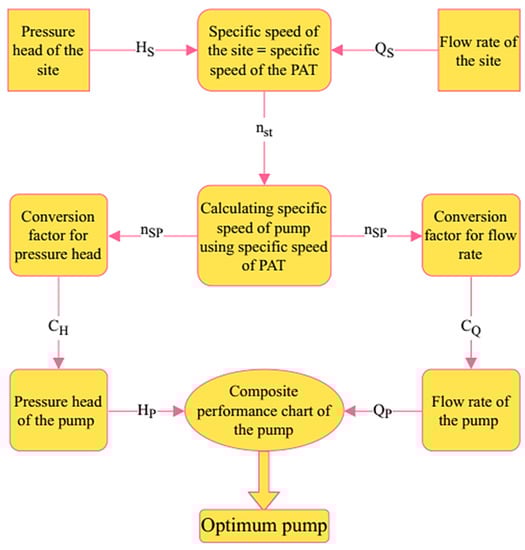
Figure 1.
Statistical model flowchart for selecting the PAT.
Table 1 presents the calculated result obtained using the statistical model and the detailed procedure described above for the selected site. According to the analysis, the recommended pump for this particular site should have a flow rate of 0.00682 m3/s (24.5 m3/h) and a head of 16.5 m at the BEP.

Table 1.
Calculation results using a statistical model.
In order to draw a general conclusion regarding the correlation between the site and pump data, the statistical procedure was repeated for an additional 12 sample sites with varying head and flow rate ranges. The head values ranged from 10 to 120 m, while the flow rates ranged from 0.0027 to 0.0333 m3/s. The relationship between the site and pump data was established using the Pearson correlation coefficient formula [27]. The simplified form of the formula is given in Equation (5).
where r is Pearson’s correlation coefficient.
∑xy is the sum of the product of the site and pump data, having the following form.
where ∑x is the total of the site data, ∑y is the total of the pump data, and n is the quantity of the information. In Equation (5), ∑x2 and ∑y2 are the sum of the square of the site and pump data and can be defined as Equations (7) and (8).
2.2. Numerical Model
In order to conduct the numerical simulation of the pump in reverse mode, several essential input parameters are required. These include the head of the pump (HP) at 16.5 m, the flow rate of the pump (QP) at 24.5 m3/h, the number of blades (Z) set to 6, and the blade tip diameter (D2), specified as 160 mm.
For estimating the performance of the pump in the reverse mode, a three-dimensional (3D) model of both the stationary and rotating parts of the pump was generated. This was achieved using the centrifugal pump design (CPD) module available in Ansys software 2022 R1 [28]. Furthermore, the impeller of the pump was further specified using BladeGen [29]. The irregular mesh was then transformed into a regular mesh with an appropriate mesh size, as illustrated in Figure 2.
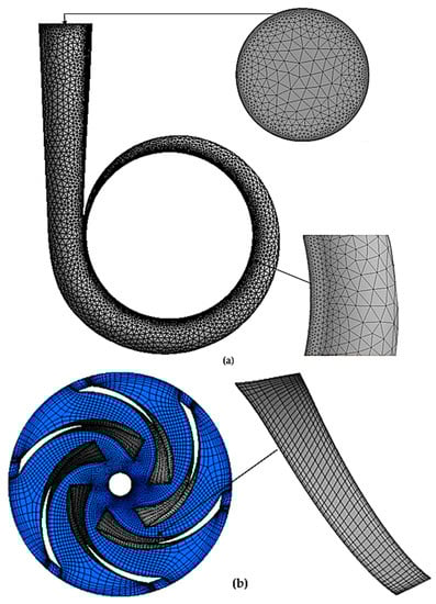
Figure 2.
Mesh refinement at sensitive areas of volute (a); impeller (b).
The stationary volute of the pump was meshed using the Ansys Mesh tool, utilizing both the unstructured and structured meshing techniques, such as Turbo-Mesh and ICEM CFD [30]. The boundary of the blade, as well as the inlet and outlet of the volute, were refined to meet the requirements of a dimensionless wall distance (y+). In addition to mesh resolution, the value of y+ is dependent on factors such as the distance from the wall to the cell center (y), fluid density (ρ), molecular viscosity (µ), and the wall shear stress (τw) (Equation (9)). For the k-ε and SST k-ω turbulence models, the near boundary wall should have a y+ value of around 200 [16] and ≤100 [16,31], respectively.
The quality of the mesh was assessed using mesh metrics, such as aspect ratio, skewness, and orthogonal quality. The individual components of the domain displayed favorable mesh quality, with an average skewness value of 0.02283 and an average orthogonal quality value of 0.98617. Furthermore, the main components exhibited an average aspect ratio of 1.1347. These values suggest that excellent mesh quality was provided across all components.
In order to assess the impact of grid size on the simulation results, six different grid numbers were used in the simulations. Among them, the fifth mesh, which consisted of 668,266 elements, was further refined by 31.5%. Despite this refinement, the results indicated only minimal deviations of approximately 0.05% and 0.06% in terms of the head and efficiency of the PAT, respectively (Figure 3). Based on these findings, a mesh size of approximately 700,000 was considered suitable for performing the numerical calculation.
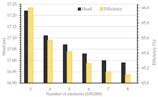
Figure 3.
A grid dependency analysis.
The physical model used in the solver employed the finite volume method with a second-order spatial discretization scheme for the convection terms in the governing equations. In the study conducted by J. Hu [31], the contribution of heat transfer was deemed negligible; thus, the energy conservation equation was not included. Thus, the continuity, Equation (10), and momentum, Equation (11), were used to govern the model, as described in [2,11].
In order to ensure the accurate convergence of the numerical simulations, a relative error criterion of less than 0.000001 was set. In addition to the standard k-ε, which is based on model transport equations for the turbulence kinetic energy (k) and its dissipation rate (ε) [2], the SST k-ω turbulence model was employed due to its ability to account for the transport of the principal shear stress within boundary layers under adverse pressure gradients [31].
In Equations (10) and (11), the variable u represents velocity (m/s), ρ represents density (kg/m3), and τij is the viscous shear stress tensor (N/m2); it is related to the strain rate via
Following the Boussinesq assumption, the Reynolds stress tensor is defined by Equation (13):
δij represents the Kronecker delta function, which is equal to one when i = j, and zero otherwise. µ is the dynamic viscosity coefficient (kg/(m·s), k represents the turbulent kinetic energy (J/kg), and µt is the turbulent eddy viscosity coefficient, defined in Equation (14):
where Cµ is a scalar function that generally depends on the strain rate and vorticity tensors [32], ε represents turbulent dissipation (m2/s3), and fu is a turbulent viscosity factor, which is defined in Equation (15).
with , where y is the distance from the wall.
In Figure 4, the first boundary condition (A) is set at a total pressure of 0 atm, while the second boundary condition (E) is defined as the mass flow rate at the outlet [2,31]. The interface between the rotor and stator is denoted as (C). The remaining boundary conditions are applied to the rotating impeller (B) and stationary volute (D). For the numerical simulation, water is chosen as the working fluid, with a temperature of 25 °C and a density of 997 kg/m3. The simulation utilizes a pressure-based solver, and an operating pressure of 101 kPa is set as the basic configuration for the numerical calculations.
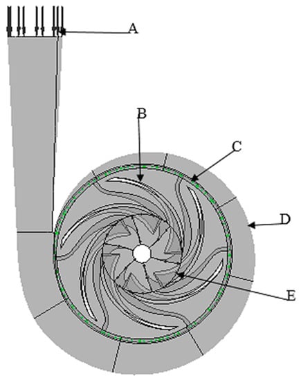
Figure 4.
Boundary conditions at the specified regions of the PAT.
2.3. Experimentation
The experimental investigation aimed to validate the accuracy of the numerical results, and its setup (Figure 5) included the following components:
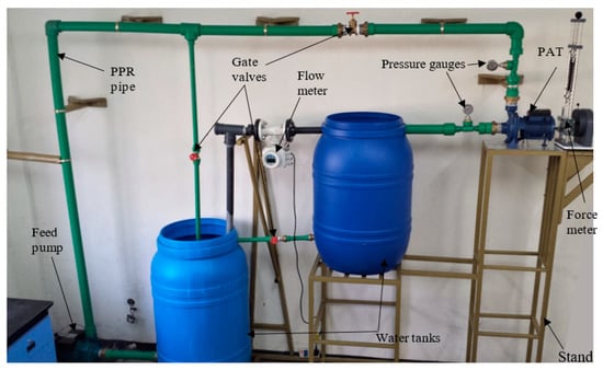
Figure 5.
Experimental setup installation.
- Pump: a pump with a power rating of 3 hp, a maximum head of 340 m, and a maximum flow rate of 30.0 m3/h was utilized to supply the required flow for the system. The inlet and outlet flange has an internal diameter of 50 mm;
- Pump as a turbine (PAT): another pump, specifically chosen to function as a turbine, was incorporated into the experimental setup. The specific parameters of this pump were described in Section 2.2 of this study. In order to ensure smooth water circulation, the PAT was positioned above the water tanks;
- Piping System: Polypropylene random copolymer (PPR) pipes were used to circulate the water in the experimental setup. A bypass pipe was installed in the system to control excess flow, and reducers and expanders were utilized to connect pipes with different diameters;
- Water Tanks: water tanks with sufficient capacity were used as water reservoirs in the experimental setup. The two tanks were connected via pipes at the sidewall to maintain an optimal water level within the primary tank;
- Flow Control: two gate valves, located in the main line and bypass pipes, were used to regulate the flow rate since the feed pump did not have its flow control mechanism.
The system was securely fixed to the wall and the ground to absorb any shock during the performance of the experiment.
The experimental test rig also included two pressure gauges with a range of 0–16 bar and an error of 0.5%, a digital flow meter with a range of 0–40 m3/h and an error of 0.4%, a tachometer with a range of 0–4000 rpm and an error of 0.05%, and a force meter with a range of 0–50 N and an error of 0.25%, which were each utilized to measure the head, flow rate, rotational speed, and force, respectively. In order to determine the total error (ES) of the measuring system, Equation (16) was employed.
where EQ is the flow meter error, EH is the pressure gauge error, En is the tachometer error, and EF is the force meter error.
After obtaining the required numerical values, the input power (pin), output power (pout), and efficiency (η) of the PATs were calculated using Equations (17)–(19):
where ρ represents the density of the fluid (kg/m3) (i.e., water at a standard condition), g is the gravitational constant (m/s2), Qt is the flow rate (m3/s), Ht is the head of the PAT (m), τ is shaft torque (N m), and ω is the angular velocity (rad/s).
In order to ensure the accuracy of the experimental data, the average of 10 repeated measurements was recorded for each parameter. Furthermore, a first-order uncertainty analysis was conducted using the constant odds combination method, which is based on a 95 percent confidence level, as described in reference [33]. The uncertainties associated with flow rate, pressure head, power, and efficiency were determined to be 3.1%, 3.2%, 2.4%, and 3.5%, respectively. These uncertainties account for the variability and potential errors in the experimental measurements.
3. Results and Discussion
3.1. Correlation between Site and Pump Hydraulic Data
The results presented in Table 2 show the relationship between the flow rate of the site (Qsite) and the pump (QP), along with other parameters, such as the specific speed of the pump (nsp), the specific speed of the PAT (nst), and the coefficient of flow rate (CQ). The data indicate a correlation between the flow rate of the site and the pump, with a coefficient of flow rate ranging from approximately 1.21–1.23.
Table 2.
The relationship between the flow rate of the site and the pump.
In a similar manner, Table 3 displays the relationship between the pressure head of the site (Hsite) and the pump (HP), along with the specific speed of the pump (nsp), specific speed of the PAT (nst), and coefficient of the head (CH). The data indicate a correlation between the pressure head of the site and the pump, with a coefficient of the head ranging approximately from 1.6–1.71.
Table 3.
The relationship between the pressure head of the site and the pump.
Based on the calculated data, generic mathematical correlations have been derived. Equation (20) represents the relationship between the site flow rate (QS) and the pump flow rate (QP), indicating that the pump flow rate is approximately 82.5% of the site flow rate. Equation (21) represents the relationship between the site head (HS) and the pump head (HP), indicating that the pump pressure head is approximately 60.5% of the site pressure head.
The correlation coefficients (highlighted in Figure 6 and Figure 7) indicate a strong positive correlation between the site and the pump data. The correlation coefficients range from 0.813 to 0.826 for the flow rate and from 0.584 to 0.625 for the pressure head. These correlation coefficients validate the practicality of the proposed correlations within the specified range of hydraulic data.
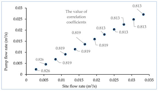
Figure 6.
Correlations between the site and pump flow rate.
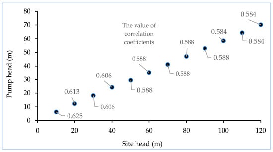
Figure 7.
Correlation between the site and pump head.
Figure 8 and Figure 9 depict the percentage of nonconformities between the step-by-step statistical model and Equations (20) and (21). The deviation between the two techniques varies across different sites. The overall accuracy of the proposed methodology is within the range of ±3.3% for the pressure head and −0.2% to +1.5% for the flow rate.
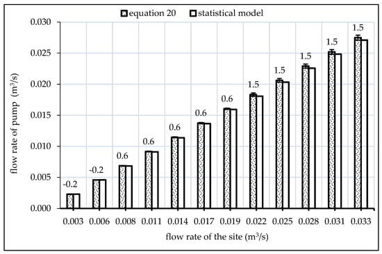
Figure 8.
The relation between the site and pump flow rate with the percentage of deviation.
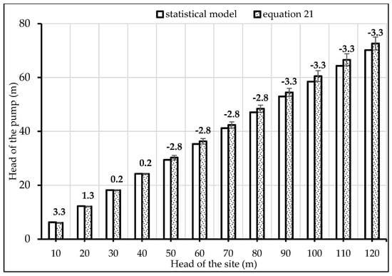
Figure 9.
The relation between the site and pump head with the percentage of deviation.
The results show that the proposed methodology is highly accurate. It is important to note that the accuracy is higher for lower hydraulic data. Considering the small deviations and the high accuracy of the proposed methodology, it can be concluded that the derived correlations provide a practical and reliable means of estimating the pump flow rate and head based on the available site hydraulic data.
3.2. Performance of the PAT
The internal flow conditions of the PAT were analyzed in terms of pressure distribution and velocity streamlining. Figure 10a shows the pressure distribution among the six blades is not uniform, indicating variation in the flow behavior. Figure 10b illustrates flow circulation and separation occurring within the PAT. In order to achieve uniform streamlines and pressure distribution, it is evident from both parameters that modifications should be made to the pump before utilizing it as a turbine. This shows the need for design improvements to optimize the performance of the PAT. After the CFD simulations, the y+ values were verified. As is shown in Figure 10c,d, the refined mesh has y+ values ranging from 0–200 for volute and from 9.517–186 for the impeller mesh, respectively. These y+ values fall within the range considered adequate for evaluating the PATs performance, as mentioned by Wang et al. [16] and Hu J. et al. [31].
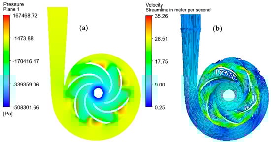
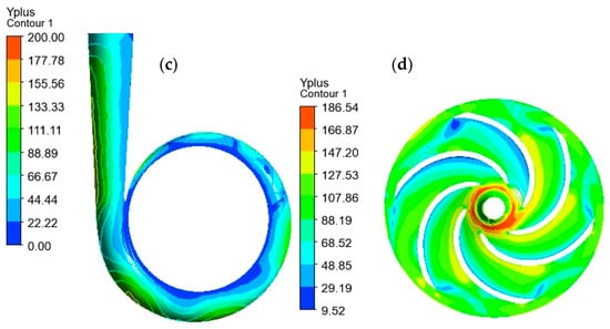
Figure 10.
Internal flow conditions; pressure (a), streamline (b), y+ volute (c), and y+ impeller (d).
By varying the flow rate of the water, the performance curves of the pump as a turbine were developed numerically as well as experimentally, as shown in Figure 11. As expected, the PAT flow rate increases with increasing pressure head and vice versa. The best efficiency values for the standard k-ε model, SST k-ω model, and experimental results were obtained at different operating points. Specifically, the highest efficiencies were observed at a head of 17.00 m, 17.75 m, and 16.5 m, flow rates of 27.50 m3/h, 28.14 m3/h, and 28.00 m3/h, and efficiency values of 65.15%, 66.67%, and 64.00%, respectively.
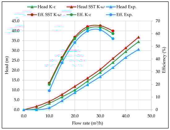
Figure 11.
Comparison of CFD and experimental value.
The simulation results obtained using the standard k-ε model show deviations from the experimental data at the best efficiency point. The deviations for flow rate, head, power, and efficiency are −1.82%, 2.94%, 2.88%, and 1.76% respectively. On the other hand, the SST k-ω model provides results with deviations of 0.49%, 7.04%, 5.10%, and 4.00% for the same parameters. Based on these deviations, it can be concluded that the standard k-ε is a suitable turbulence model for the analysis of the pump running as a turbine. It should be noted that numerical errors are inherent in simulations due to approximations of natural laws and the consideration of only hydraulic losses. Table 4 summarizes a comparison between the numerical results of the two turbulence models and the experimental values.
Table 4.
Comparison of standard k-ε and SST k-ω results with experimental value at the best efficiency point.
Furthermore, Figure 12 illustrates the percentage of deviation (error) in the numerical results compared to the experimental data from various studies, including Si. Huang et al. [34], Sun-Sheng Yang et al. [35], Yang Sun-Sheng et al. [36], Y. Sun-Sheng et al. [37], and Shi H.X. et al. [38]. The numerical predictions for the head, output power, and efficiency show good agreement with the experimental data. The average absolute error between the numerical and experimental results for head, power, and efficiency from various published works is also provided, demonstrating that the numerical model falls within an acceptable range. The deviation between the numerical and experimental results is potentially due to differences in the software type, mesh size, turbulence model, physics setup, and experimental equipment used in different studies.
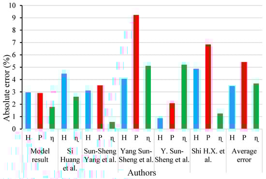
Figure 12.
Comparison of model results with other methods (%) [34,35,36,37,38].
4. Conclusions
In conclusion, this research work focuses on the selection and performance analysis of the pump as a turbine. A selection chart and statistical model are adopted to select the optimum pump for specific working conditions. Mathematical correlations were developed to establish the relationship between the site and the pump hydraulic data. Ansys CFX, coupled with standard k-ε and SST k-ω, was used to predict the performance of the PAT. Then, the numerical outputs were validated using an experimental result. The following key conclusions were drawn from the study.
- The proposed correlations enable the selection of the optimal pumps for power generation applications. The developed method exhibited high accuracy, with deviations of −0.2% to +1.5% for flow rate and ±3.0% for head;
- The deviations between the CFD results and experimental data at the best efficiency point were determined. The standard k-ε model exhibited deviations of −1.82%, 2.94%, 2.88%, and 1.76% for flow rate, head, power, and efficiency, respectively. The SST k-ω model showed deviations of 0.49%, 7.04%, 5.10%, and 4.00% for the same parameters. Based on these, the standard k-ε model was found to be more suitable for analyzing the performance of pumps operating as turbines;
- In general, the adopted numerical procedure, selected mesh type, turbulence model, and physics setup provided good agreement with the experimental result;
- Future research directions could focus on introducing new modification techniques to further improve the performance of pumps operating as turbines. This could help maximize the performance of pumps used in power generation applications.
Author Contributions
Conceptualization, A.N. and E.D.; supervision, E.D. and M.G.; data curation, A.N.; methodology, A.N., E.D. and M.G.; formal analysis, H.B.M.; simulation, A.N. validation, A.N. and M.G. writing-original draft preparation, A.N., M.G. and H.B.M.; writing-reviewing and editing, M.G. and H.B.M.; funding acquisition, M.G. and H.B.M. All authors have read and agreed to the published version of the manuscript.
Funding
This research was funded by the Addis Ababa Science and Technology University (AASTU) under internal research grants (Grant No. EM-229/19-1/21).
Data Availability Statement
The data that support the findings of this study are available within the article.
Conflicts of Interest
The authors declare no conflict of interest.
References
- Tucho, G.T.; Nonhebel, S. Alternative energy supply system to a rural village in Ethiopia. Energy Sustain. Soc. 2017, 7, 33. [Google Scholar] [CrossRef]
- Nasir, A.; Dribssa, E.; Girma, M.; Demeke, T. A Comparative Study of Impeller Modification Techniques on the Performance of the Pump as a Turbine. Int. J. Rotating Mach. 2022, 2022, 1944753. [Google Scholar] [CrossRef]
- Kramer, M.; Terheiden, K.; Wieprecht, S. Pumps as turbines for efficient energy recovery in water supply networks. Renew. Energy 2018, 122, 17–25. [Google Scholar] [CrossRef]
- Jemal, A.N.; Haile, M.G. Comprehensive Review of Pump as Turbine (PAT). Renew. Energy Sustain. Dev. 2019, 5, 68–100. [Google Scholar] [CrossRef]
- Rakibuzzaman, M.; Jung, K.Y.; Suh, S.H. A study on the use of existing pump as turbine. E3S Web Conf. 2019, 128, 06004. [Google Scholar] [CrossRef]
- Buono, D.; Frosina, E.; Mazzone, A.; Cesaro, U.; Senatore, A. Study of a Pump as Turbine for a hydraulic urban network using a tridimensional CFD modeling methodology. Sci. Energy Procedia 2015, 82, 201–208. [Google Scholar] [CrossRef]
- Slocum, A.H.; Haji, M.N.; Trimble, A.Z.; Ferrara, M.; Ghaemsaidi, S.J. Integrated Pumped Hydro Reverse Osmosis systems. Sustain. Energy Technol. Assess. 2016, 18, 80–99. [Google Scholar] [CrossRef]
- Chacón, M.C.; Díaz, J.A.R.; Morillo, J.G.; McNabola, A. Pump-as-turbine selection methodology for energy recovery in irrigation networks: Minimising the payback period. Water 2019, 11, 149. [Google Scholar] [CrossRef]
- Liu, M.; Tan, L.; Cao, S. Performance Prediction and Geometry Optimization for Application of Pump as Turbine: A Review. Front. Energy Res. 2022, 9, 818118. [Google Scholar] [CrossRef]
- De Marchis, M.; Milici, B.; Volpe, R.; Messineo, A. Energy saving in water distribution network through pump as turbine generators: Economic and environmental analysis. Energies 2016, 9, 877. [Google Scholar] [CrossRef]
- Cao, Z.; Deng, J.; Zhao, L.; Lu, L. Numerical research of pump-as-turbine performance with synergy analysis. Processes 2021, 9, 1031. [Google Scholar] [CrossRef]
- Simão, M.; Pérez-Sánchez, M.; Carravetta, A.; Ramos, H.M. Flow conditions for PATS operating in parallel: Experimental and numerical analyses. Energies 2019, 12, 901. [Google Scholar] [CrossRef]
- Bozorgi, A.; Javidpour, E.; Riasi, A.; Nourbakhsh, A. Numerical and experimental study of using axial pump as turbine in Pico hydropower plants. Renew. Energy 2013, 53, 258–264. [Google Scholar] [CrossRef]
- Hu, J.; Su, W.; Li, K.; Wu, K.; Xue, L.; He, G. Transient Hydrodynamic Behavior of a Pump as Turbine with Varying Rotating Speed. Energies 2023, 16, 2071. [Google Scholar] [CrossRef]
- Frosina, E.; Buono, D.; Senatore, A. A Performance Prediction Method for Pumps as Turbines (PAT) Using a Computational Fluid Dynamics (CFD) Modeling Approach. Energies 2017, 10, 103. [Google Scholar] [CrossRef]
- Wang, X.; Yang, J.; Xia, Z.; Hao, Y.; Cheng, X. Effect of Velocity Slip on Head Prediction for Centrifugal Pumps as Turbines. Math. Probl. Eng. 2019, 2019, 5431047. [Google Scholar] [CrossRef]
- Sambito, M.; Piazza, S.; Freni, G. Stochastic approach for optimal positioning of pumps as turbines (Pats). Sustainability 2021, 13, 2318. [Google Scholar] [CrossRef]
- Miao, S.; Yang, J.; Shi, F.; Wang, X.; Shi, G. Research on energy conversion characteristic of pump as turbine. SAGE J. 2018, 10, 1687814018770836. [Google Scholar] [CrossRef]
- Li, D.; Sun, Y.; Zuo, Z.; Liu, S.; Wang, H.; Li, Z. Analysis of pressure fluctuations in a prototype pump-turbine with different numbers of runner blades in turbine mode. Energies 2018, 11, 1474. [Google Scholar] [CrossRef]
- Barbarelli, S.; Amelio, M.; Florio, G.; Scornaienchi, N.M. Procedure Selecting Pumps Running as Turbines in Micro Hydro Plants. Energy Procedia 2017, 126, 549–556. [Google Scholar] [CrossRef]
- Yang, S.; Li, P.; Lu, Z.; Xiao, R.; Zhu, D.; Lin, K.; Tao, R. Comparative evaluation of the pump mode and turbine mode performance of a large vaned-voluted centrifugal pump. Front. Energy Res. 2022, 10, 1003449. [Google Scholar] [CrossRef]
- Nasir, A. Design and Simulation of Photo-voltaic Water Pumping System for Irrigation. Adv. Appl. Sci. 2019, 4, 59. [Google Scholar] [CrossRef]
- Amelio, M.; Barbarelli, S.; Schinello, D. Review of methods used for selecting Pumps as Turbines (PATs) and predicting their characteristic curves. Energies 2021, 13, 6341. [Google Scholar] [CrossRef]
- Morani, M.C.; Carravetta, A.; Del Giudice, G.; McNabola, A.; Fecarotta, O. A comparison of energy recovery by pATs against direct variable speed pumping in water distribution networks. Fluids 2018, 3, 41. [Google Scholar] [CrossRef]
- Mdee, O.J.; Kimambo, C.Z.; Nielsen, T.K.; Kihedu, J. Methodological approach of performance evaluation for using pump as micro hydro-turbine. In Proceedings of the ISES Solar World Conference 2017 and the IEA SHC Solar Heating and Cooling Conference for Buildings and Industry, Abu Dhabi, United Arab Emirates, 29 October–2 November 2017; pp. 46–57. [Google Scholar] [CrossRef]
- Chapallaz, P.J.M.; Eichenberger, G.F. Manual on Pumps Used as Turbines; Viewing and Sohn Verlagsgesellschaft mbH: Braunschweig, Germany, 1992. [Google Scholar]
- Zinzendoff Okwonu, F.; Laro Asaju, B.; Irimisose Arunaye, F. Breakdown Analysis of Pearson Correlation Coefficient and Robust Correlation Methods. IOP Conf. Ser. Mater. Sci. Eng. 2020, 917, 012065. [Google Scholar] [CrossRef]
- Alawadhi, K.; Alzuwayer, B.; Mohammad, T.A.; Buhemdi, M.H. Design and optimization of a centrifugal pump for slurry transport using the response surface method. Machines 2021, 9, 60. [Google Scholar] [CrossRef]
- Kim, B.; Siddique, M.H.; Samad, A.; Hu, G.; Lee, D.E. Optimization of Centrifugal Pump Impeller for Pumping Viscous Fluids Using Direct Design Optimization Technique. Machines 2022, 10, 774. [Google Scholar] [CrossRef]
- Liu, M.; Tan, L.; Cao, S. Theoretical model of energy performance prediction and BEP determination for centrifugal pump as turbine. Energy 2019, 172, 712–732. [Google Scholar] [CrossRef]
- Hu, J.; Su, X.; Huang, X.; Wu, K.; Jin, Y.; Chen, C.; Chen, X. Hydrodynamic Behavior of a Pump as Turbine under Transient Flow Conditions. Processes 2022, 10, 408. [Google Scholar] [CrossRef]
- Newman, J.; Bangga, G.; Kusumadewi, T.; Hutomo, G.; Sabila, A. Improving a two-equation eddy-viscosity turbulence model to predict the aerodynamic performance of thick wind turbine airfoils. IOP Conf. Ser. J. Phys. Conf. Ser. 2018, 974, 012019. [Google Scholar]
- Kline, S.J. The purposes of uncertainty analysis. J. Fluids Eng. Trans. ASME 1985, 107, 153–160. [Google Scholar] [CrossRef]
- Huang, S.; Qiu, G.; Su, X.; Chen, J.; Zou, W. Performance prediction of a centrifugal pump as turbine using rotor-volute matching principle. Renew. Energy 2017, 108, 64–71. [Google Scholar] [CrossRef]
- Yang, S.S.; Derakhshan, S.; Kong, F.Y. Theoretical, numerical and experimental prediction of pump as turbine performance. Renew. Energy 2012, 48, 507–513. [Google Scholar] [CrossRef]
- Yang, S.S.; Kong, F.Y.; Jiang, W.M.; Qu, X.Y. Effects of impeller trimming influencing pump as turbine. Comput. Fluids 2012, 67, 72–78. [Google Scholar] [CrossRef]
- Sun-Sheng, Y.; Fan-Yu, K.; Jian-Hui, F.; Ling, X. Numerical research on effects of splitter blades to the influence of pump as turbine. Int. J. Rotating Mach. 2012, 2012, 123093. [Google Scholar] [CrossRef]
- Shi, H.X.; Chai, L.P.; Su, X.Z.; Jaini, R. Performance optimization of energy recovery device based on PAT with guide vane. Int. J. Simul. Model. 2018, 17, 472–484. [Google Scholar] [CrossRef]


Disclaimer/Publisher’s Note: The statements, opinions and data contained in all publications are solely those of the individual author(s) and contributor(s) and not of MDPI and/or the editor(s). MDPI and/or the editor(s) disclaim responsibility for any injury to people or property resulting from any ideas, methods, instructions or products referred to in the content. |
© 2023 by the authors. Licensee MDPI, Basel, Switzerland. This article is an open access article distributed under the terms and conditions of the Creative Commons Attribution (CC BY) license (https://creativecommons.org/licenses/by/4.0/).