Photovoltaic Energy Forecast Using Weather Data through a Hybrid Model of Recurrent and Shallow Neural Networks

Abstract

In this article, forecast models based on a hybrid architecture that combines recurrent neural networks and shallow neural networks are presented. Two types of models were developed to make predictions. The first type consisted of six models that used records of exported active energy and meteorological variables as inputs. The second type consisted of eight models that used meteorological variables. Different metrics were applied to assess the performance of these models. The best model of each type was selected. Finally, a comparison of the performance between the selected models of both types was presented. The models were validated using real data provided by a solar plant, achieving acceptable levels of accuracy. The selected model of the first type had a root mean square error (RMSE) of 0.19, a mean square error (MSE) of 0.03, a mean absolute error (MAE) of 0.09, a correlation coefficient of 0.96, and a determination coefficient of 0.93. The other selected model of the second type showed lower accuracy in the metrics: RMSE = 0.24, MSE = 0.06, MAE = 0.10, correlation coefficient = 0.95, and determination coefficient = 0.90. Both models demonstrated good performance and acceptable accuracy in forecasting the weekly photovoltaic energy generation of the solar plant.

1. Introduction

Photovoltaic energy has experienced remarkable growth worldwide due to increasing energy demand and the imperative to reduce greenhouse gas emissions. In both the industrial and residential sectors, this renewable energy source meets the needs of large consumers and promotes decentralized electricity production in homes, thereby reducing reliance on non-renewable sources and fostering a sustainable energy model. Photovoltaic energy generation stands out for its capacity to mitigate CO₂ emissions, positioning it as an effective and expanding solution in the fight against climate change and the transition towards a cleaner and more sustainable energy future [1,2].

The proliferation of photovoltaics has brought forth a range of challenges that necessitate attention and innovative solutions. One pertinent issue is associated with the intermittent and volatile nature of energy generation in photovoltaic systems, which is directly influenced by weather conditions such as solar radiation, cloud cover, and seasonal variations. The availability and intensity of sun radiation significantly impact photovoltaic energy generation. Although solar panels convert sun radiation into electrical energy during the day, this generation can fluctuate considerably due to climatic changes [3].

This volatility can lead to imbalances in the photovoltaic system, and they impact the stability of the integrated electrical grid. In large-scale solar plants, particularly those connected to the power grid, these unforeseen fluctuations can cause significant swings in power generation, resulting in power quality issues and supply disruptions [4]. Apart from the technical and system stability challenges, the volatility of photovoltaic generation also carries economic implications. Large solar plants typically operate based on long-term power supply contracts, and any unanticipated variation in generation can lead to contract violations and substantial financial losses [5].

To tackle this issue, several solutions have been developed. One of these solutions involves the utilization of short-term forecast models. These models enable the monitoring and forecast of photovoltaic energy generation based on weather conditions and other pertinent factors. By employing machine learning techniques, these models provide more precise forecasts, thereby aiding in the optimization of solar plant operations and mitigating the adverse effects of generation volatility. The pursuit of technological solutions is pivotal in alleviating the negative impacts associated with such volatility, ensuring the efficient integration of photovoltaic energy into the power grid and fostering the sustainable development of this significant renewable energy source [6].

Solar plants regularly measure and record the daily exported active energy (EAE) generated by their photovoltaic panels. These plants typically have weather stations that capture important climatic variables. By combining these data, solar plants can monitor their production and examine the relationship between the generated EAE and local weather conditions. However, meteorological variables inherently exhibit volatility and uncertainty, which means that unexpected fluctuations in these parameters can lead to variations in the power output of photovoltaic systems.

Despite the research efforts made in recent years to develop innovative models that can predict meteorological variables relevant to photovoltaic generation, an essential step is often overlooked: the exploratory analysis of the data before its utilization. This analysis provides a comprehensive understanding of the data’s characteristics and patterns, yielding valuable insights to enhance forecast models and attain more accurate and dependable results.

Accurate forecasting of photovoltaic power generation is essential for ensuring efficient operation of solar plants. Enhancing the precision of short-term forecasts has significant benefits, including supporting the quality of operational schedules, providing guidance for photovoltaic maintenance, and enabling effective response to emergency situations. Typically, the data sources used for such forecasts include weather records, numerical weather forecasts, and historical records of EAE generated by the solar plant [6].

In recent literature, comparative studies have been conducted on recurrent neural networks (RNN) with various structural configurations, input hyperparameters, and prediction horizons [7]. Additionally, there are research efforts focused on generating forecast models for photovoltaic energy, which can be broadly categorized into three groups:

• Machine learning techniques: use artificial neural networks (ANN), RNN, support vector machines (SVM), and genetic algorithm (GA) techniques.
• Statistical techniques: includes forecast models based on statistical techniques such as regression analysis, Bayesian networks, time series analysis, autoregressive integrated moving average (ARIMA), and autoregressive moving average (ARMA) models.
• Hybrid approaches: hybrid models combine elements of statistical methods, machine learning techniques, and physical models.

While many studies in the field of photovoltaic energy forecasting primarily utilize machine learning techniques, particularly RNNs, due to their effectiveness in processing time series data, it is worth highlighting the significance of initiatives that explore the development and utilization of hybrid models for predicting photovoltaic energy production.

In terms of model validation techniques, the majority of reviewed works tend to focus on a single metric, such as the root mean square error (RMSE). There are other important metrics that are often considered secondary. These metrics include mean square error (MSE), mean absolute error (MAE), mean absolute percentage error (MAPE), and Pearson’s correlation coefficient. Additionally, these studies typically do not utilize large volumes of data for training and validating their models [7,8,9].

Extreme weather conditions pose a challenge for accurate photovoltaic energy forecasts, as they can result in intermittent and unpredictable volatility in photovoltaic systems. While RNN models are effective for forecasting time-series data, they may encounter difficulties when confronted with abrupt long-term climate changes. These changes can cause the gradient to vanish during the training process of an RNN, leading to suboptimal forecasts.

In such situations, it is crucial to carefully consider the limitations and potential drawbacks of RNN models. Alternative approaches or modifications to the traditional RNN architecture, such as long short-term memory (LSTM) or gated recurrent unit (GRU) models, may offer better performance and more robust forecasts in the face of extreme weather events and long-term climate changes [9,10].

In this article, the focus is on the development of forecast models for the generation of photovoltaic energy. It uses a base architecture described in a previous research work, referred to as [11]. This hybrid architecture combines RNN and ANN components in two hidden layers:

• The first layer contains neurons with LSTM or GRU recurrent units.
• The second layer is composed of shallow neurons with a multilayer perceptron (MLP) structure.

Although this hybrid RNN–ANN architecture had already been used in the aforementioned work, it only generated forecast models with a single input variable. However, in this paper, multiple input variables are utilized in the models, and different hyperparameter configurations are explored. The input variables consist of historical EAE records and measurements of weather variables, including solar radiation, temperature, and wind speed, taken throughout one year. The hyperparameters are associated with the internal components of the model, including the activation function and the loss function, among others.

Two types of models are configured. First, six models are developed that receive the EAE records along with the weather variables as input. Second, eight models are created that only use weather variables as input. Both types of models achieve good accuracy in forecasting photovoltaic energy generation. The models with the best performance indicators of each type are selected by analyzing five metrics: RMSE, MSE, MAE, correlation coefficient, and determination coefficient. This process is accomplished through controlled experiments and the optimization of various hyperparameter configurations. Finally, the two models with the best performance of each type are compared. The results show that the models using the EAE records along with the weather variables as input exhibit better performance in most of the metrics.

The contributions of the results of this work are as follows:

• By using multiple variables as input in the generated models, the validation of the efficient performance of the RNN–ANN hybrid architecture allows us to project the improvement of the forecast models. This is because we can incorporate new variables related to internal factors of the photovoltaic panels and other physical features in subsequent works.
• The implementation, configuration, and generation of a wide variety of photovoltaic energy forecast models through the RNN–ANN hybrid architecture.
• The general implementation of models based on the RNN–ANN hybrid architecture stands out for its simplicity, flexibility, and applicability in various contexts, such as wind energy forecasting or others, provided that the data sets are prepared as input sequences for time series.

In relation to the primary studies reviewed in the related works section, this work distinguishes itself through the following contributions:

• It provides a hybrid approach for generating forecast models, utilizing both univariable and multivariable inputs. This approach can be further discussed to improve its performance or combined with other RNN structures.
• It evaluates the performance of forecast models using five metrics. This allows for an analysis of the models’ performances from different perspectives, thereby strengthening the evaluation stage.

The article is structured as follows: the “Related Works” section provides a literature review of the past five years, focusing on studies directly related to this work. This review allows us to corroborate the innovation of the work carried out and the use of appropriate techniques and metrics. The “Materials and Methods” section describes the data source, the methodology used, the preliminary analysis of the data, as well as its preparation and transformation. Additionally, the tool built and used to automate the entire process of design and generation of predictive models is explained. The “RNN–ANN Models” section presents the model design, hyperparameter configuration, and metrics used for their assessment. Subsequently, the “Analysis of Experimental Results” section provides a discussion of the results obtained through the selected models and performs a comparative analysis. Finally, the article ends by stating the respective conclusions obtained from the work carried out, as well as projections for future work. Table 1 below presents the list of abbreviations used in this work.

Table 1. Abbreviation list.

Abbreviation	Meaning	Abbreviation	Meaning
ANN	Artificial neural network	CO2	Carbon dioxide
RNN	Recurrent neural network	EAE	Active energy exported
CNN	Convolutional neural network	SVM	Support vector machine
LSTM	Long short-term memory	GA	Genetic algorithm
GRU	Gated recurrent units	IRRAD	Radiation
MLP	Multi-layer perceptron	TEMP	Temperature
BiLSTM	Bidirectional long short-term memory	WS1	Wind speed
RMSE	Root mean square error	WANG	Wind angle
MSE	Mean square error	KWh	Kilowatt hour
MAE	Mean absolute error	°C	Degree Celsius
MAPE	Mean absolute percentage error	W/m2	Watt per square meter
ARMA	Autoregressive moving average	MW	Megawatts
ARIMA	Autoregressive integrated moving average	CSV	Comma-separated values
SARIMA	Seasonal autoregressive integrated moving average	API	Application programming interface

2. Related Works

The worldwide growth in the use of photovoltaic energy has driven the development of various research initiatives aimed at obtaining high-precision models to forecast its generation. Due to this, the present research work begins with a bibliographical review of related works in this field in recent years to confirm which methodologies as well as techniques are at the forefront of research.

Yesilbudak et al. [3] provided a bibliographic review of a methodology for the data mining process for the forecast of electricity generation in solar plants. They presented a general data analysis process. As a result, they returned a table that lists different investigations that are referenced and points out the data that they use as input, as well as the model used for the prediction. Many of the works analyzed use ANN techniques.

The work of Maciel et al. [12], evaluates the forecast accuracy of the global horizontal irradiance, which is often used in short-term forecasts of solar radiation. The study uses ANN models with different construction structures and input weather variables to forecast photovoltaic energy production across three short-term forecast horizons using a single database. The analyses were conducted in a controlled experimental environment. The results indicate that ANNs using the global horizontal irradiance input variable provide higher accuracy (approximately 10%), while their absence increases error variability. No significant differences $(p>0.05)$ were identified in the forecast error models trained with different input data sets. Furthermore, forecast errors were similar for the same ANN model across different forecast horizons. The 30 and 60-neuron models with one hidden layer demonstrated similar or higher accuracy compared to those with two hidden layers.

In [13], a study is described that uses a time-frequency analysis based on short waveforms of data combined with an RNN to forecast sun irradiation in the next 10 min. This validation allows the amount of photovoltaic energy that is generated to be estimated. The validation results indicate that this forecast model has a deviation of less than 4% in 90.60% of the sample days analyzed. The MSE of the final model improved accuracy by 37.52% compared to the persistence reference model.

Carrera et al. [14] proposed the use of RNNs to forecast photovoltaic energy generation. They designed two types of RNNs: one using weather forecast data, and one using recent weather observations. Then, they combined both networks into PVHybNet, a hybrid network. The final model was successful in predicting photovoltaic energy generation at the Yeongam Solar Plant in South Korea, with an r² value of 92.7%. These results support the effectiveness of the combined network, which uses weather observations and forecasts. It also outperformed other machine learning models.

In the article of Rosato et al. [15], a new deep learning approach was proposed for the predictive analysis of energy-related time series trends, particularly those relevant to photovoltaic systems. The objective was to capture the trend of the time series; that is, if the series increases, decreases, or remains stable, instead of predicting the future numerical values. The modeling system is based on a RNN of a LSTM structure, which are capable of extracting information in samples located very far from the current one. This new approach has been tested in a real-world case study, showing good robustness and accuracy.

The work described in [16] uses an LSTM-based approach for short-term forecasts of global horizontal irradiance. Previous ANN and SVR results have demonstrated that they are inaccurate on cloudy days. To improve the accuracy on these days, the k-means clustering technique was used during data processing to classify the data into two categories: cloudy and mixed. RNN models were compared to assess different approaches, and an interregional study was conducted to assess their generalizability. The results showed that the r² coefficient of LSTM on cloudy and mixed days exceeded 0.9, while RNN only reached 0.70 and 0.79 in Atlanta and Hawaii, respectively. In the daily forecasts, all r² values on cloudy days were approximately 0.85. It was concluded that LSTM significantly improved accuracy compared to the other models.

The article by Hui et al. [17] proposed a hybrid learning method for weekly photovoltaic energy forecasting, utilizing weather forecast records and historical production data. The proposed algorithm combined bi-cubic interpolation and bi-directional LSTM (BiLSTM) to increase the temporal resolution of weather forecast data from three hours to one hour and improve forecast accuracy. Furthermore, a weekly photovoltaic energy classification strategy based on meteorological processes was established to capture the coupling relationships between weather elements, continuous climate changes, and weekly photovoltaic energy. The authors developed a scenario forecast method based on a closed recurrent unit GRU and a convolutional neural network (CNN) to generate weekly photovoltaic energy scenarios. The evaluation indices were presented to comprehensively assess the quality of the generated scenarios. Finally, the proposed method was validated using photovoltaic energy power records, observations, and meteorological forecasts collected from five solar plants in Northeast Asia to demonstrate its effectiveness and correctness.

In the study conducted by Xu et al. [18], the current state of research on renewable energy generation and predictive technology for wind and photovoltaic energy was described. The authors proposed a short-term forecast model for multivariable wind energy using the LSTM sequential structure with an optimized hidden layer topology. They evaluated physical models, statistical learning methods, and machine learning approaches based on historical data for wind and photovoltaic energy production forecasting. They examined the impact of cloud map identification on photovoltaic generation and focused on the impact of renewable energy generation systems on electrical grid operation and its causes. The article provided a summary of the classification of wind and photovoltaic power generation systems, as well as the advantages and disadvantages of photovoltaic systems and wind power forecasting methods based on various typologies and analysis methods.

In the article by Nkambule et al. [19], the authors introduced nine maximum power point tracking techniques for photovoltaic systems. These techniques were used to maintain the photovoltaic element array at its maximum power point and extract the maximum power available from the arrays. The authors evaluated and tested these techniques under different climatic conditions using the simulation software MATLAB SIMULINK. The tested machine learning algorithms included a decision tree, multivariate linear regression, Gaussian process regression, k-weighted nearest neighbors, linear discriminant analysis, packed tree, Naive Bayes classifier, support vector machine (SVM), and RNN. The experimental results showed that the k-weighted nearest neighbors technique performed significantly better compared to the other machine learning algorithms.

One interesting study related to the analyzed topic is presented in [20], which proposed an improved deep learning model based on the decomposition of small wavelet data for the prediction of solar irradiance the next day. The model uses CNN and LSTM and was established separately for four general types of climates (sunny, cloudy, rainy, and heavy rainy) due to the high dependence of sun radiation on weather conditions. For certain weather types, the raw solar irradiance sequence is decomposed into sub-sequences using discrete wavelet transformation. Each sub-sequence is then fed of a local CNN-based feature extractor to learn its abstract representation automatically. As the extracted features were also time-series data, they were individually input into LSTM to build the sub-sequence forecasting model. The final results of solar irradiance forecast for each weather type were obtained through the reconstruction of the small wavelet data of these forecast sub-sequences. The proposed method was compared with traditional deep learning models and demonstrated an improved predictive accuracy.

The article by Alkandari and Ahmand [21] describes the task of forecasting photovoltaic energy generation from weather variables such as solar radiation, temperature, precipitation, wind speed, and direction. The authors analyzed different techniques to determine the most suitable for photovoltaic energy forecasting. They proposed an approach that combined different techniques based on RNN models and statistical models based on their experimental results.

In [22], a data analysis process was developed to evaluate the performance of a predictive model generated using a database containing information on historical data of the energy produced. They highlighted the importance of performing good data preprocessing through various tasks in the initial stage of the work. They showed forecasts at different time horizons using ANN implementations, which have been used to solve similar problems in the past. First, they evaluated the interaction between anomaly detection techniques and predictive model accuracy. Second, after applying three performance metrics, they determined which one was the best for this particular application.

The research by Harrou et al. [23] proposed a model based on RNN with LSTM structure for the short-term prediction of photovoltaic energy production. The model was evaluated using records of power generation in 24-h segments, using data from a solar plant. The authors described the model used and highlighted its good performance during the training stage. In further development, they indicated their intention to incorporate weather variables into the model to further improve the model results.

The work of De et al. [24] proposed photovoltaic energy forecast models using RNNs with LSTM units. Limited datasets of one month were used with a frequency of 15 min. The goal was to achieve accurate forecasts with the LSTM framework. The results showed high precision, even with limited data, and in a reasonable amount of time. The hyperparameters were optimized, and variables such as temperature, panel temperature, stored energy, radiation, and output power were used.

In the work of Chen et al. [25], the authors analyzed the effects of various meteorological factors on the generation of photovoltaic energy and their impact during different periods. They proposed a simple radiation classification method based on the characteristics of the radiation records, which helps in selecting similar time periods. They employed the time series characteristic of photovoltaic energy production records to reconstruct the training dataset in a given period, which included output power and weather data. They presented the development of an RNN model with neurons in a LSTM structure, which was applied to data from two photovoltaic systems. The forecast results of this model stood out when they were compared to four other models.

The work of Sharadga et al. [26] evaluated various RNN models for forecasting photovoltaic energy output power using time series. Statistical techniques such as ARMA, ARIMA, and SARIMA were compared with RNN models and their variants, such as LSTM, BiLSTM, recurrent layer, direct RNN, MLP, and c-mean fuzzy clustering. The impact of the time horizon on the forecasts was analyzed, and hourly forecasts were made using data from a photovoltaic power station in China with a total of 3640 operating hours.

The study by Rajagukguk et al. [27] analyzed deep learning models for predicting solar radiation and photovoltaics in a time series. They compared four models: RNN, LSTM, GRU, and CNN–LSTM, considering accuracy, input data, forecast horizon, station type, weather, and training time. The results showed that each model had strengths and limitations under different conditions. LSTM stood out, with the best performance in terms of RMSE. The CNN–LSTM hybrid model outperformed the independent models, although it required more training time. Deep learning models are better suited to predict solar radiation and photovoltaics than conventional machine learning models. It is recommended to use the relative RMSE as a proxy metric to compare accuracy between models.

In the study provided by ref. [28], a methodology based on spectral irradiances and GA was presented to analyze the performance of photovoltaic modules. It was observed that the power conversion efficiency of these modules can vary, even under the same solar radiation. A case study was carried out in Malaysia, where twelve types of commercial photovoltaic modules were selected to simulate their conversion efficiencies and annual energy yields. This methodology provides detailed information on local spectral radiations and photovoltaic energy specifications, allowing for accurate analysis of module performance.

The work cited in [29] presents a methodology to calculate the energy conversion efficiency in organic photovoltaic cells by means of indoor measurements. A solar simulator and the measured local solar spectrum were used, considering optical and electrical factors. As a case study, random data of local solar spectra was collected throughout the year in Malaysia from 8:00 a.m. to 5:00 p.m. or 6:00 p.m. This analysis provides guidance for selecting the proper organic materials in solar cells and optimizing their performance at specific locations.

The study conducted by Jaber et al. [30] presented a forecast model based on a generalized regression ANN to compare the performance of six photovoltaic modules. Using variables such as cell temperature, irradiance, fill factor, peak power, short circuit current, open circuit voltage, and the product of the last two variables, 37,144 records from 247 module curves were collected under various climatic conditions in Malaysia. The results obtained showed a high precision in the prediction of the performance of the photovoltaic modules.

In the work of Diouf et al. [31], the impact of the operating temperature on the performance of photovoltaic modules was analyzed. A temperature forecast model was developed using ambient temperature and solar irradiance data obtained in a tropical region. The proposed approach captured the temperatures of the photovoltaic modules in different weather conditions, and they were compared with the experimentally measured values. The results showed that the proposed models outperformed those developed by other authors in terms of accuracy, which was evaluated using the MSE metric.

Bevilacqua et al. [32] investigated the effect of sun radiation on the temperature of photovoltaic panels. They proposed a one-dimensional finite-difference thermal model to calculate the temperature distribution within the panel and predict electricity production under various climatic conditions. The results revealed that, although the temperature could be predicted with high accuracy, the accuracy in predicting the power output varied. The model was validated using one year of experimental data at the University of Calabria, demonstrating excellent agreement between power predictions and actual measurements.

In the work of Zhang et al. [33], the influence of factors on photovoltaic energy forecasting was analyzed using ANN surface and small wave models. The effects of atmospheric temperature, relative humidity, and wind speed on polysilicon and amorphous silicon cells were examined. The experimental results revealed that atmospheric temperature had the highest correlation with output power in polysilicon cells, followed by wind speed and relative humidity. For amorphous silicon cells, relative humidity showed the highest correlation, followed by atmospheric temperature and wind speed.

He et al. [34] presented a forecast model for photovoltaic energy generation that uses a BiLSTM structure in an RNN. They selected the weather factors that affected energy generation using the Pearson correlation coefficient. Then, the design and implementation of the proposed model were detailed and evaluated using real data collected from a solar plant in China. The experimental results confirmed that the model had the low forecast error and highest accuracy of fit than the other tested models, such as SVR, decision tree, random forest, and LSTM.

Chen and Chang [35] proposed a method to forecast photovoltaic energy based on an RNN with a LSTM structure. They used Pearson’s correlation coefficients to analyze the influence of external conditions on the variation of photovoltaic energy and eliminate irrelevant characteristics. The results of the case study showed that sun radiation, temperature, and humidity played a decisive role in this variation. Compared with conventional ANN algorithms, such as a radial basis ANN function and time series, the proposed method demonstrated superior performance in terms of accuracy.

In the work of Konstantinou et al. [36], an RNN model was evaluated to forecast photovoltaic energy generation 1.5 h in advance. Using the historical production records of a solar plant in Cyprus as input, the model was defined and trained. Performance evaluation was performed using graphical tools, calculating the RMSE metric, and applying cross-validation. The results showed that the proposed model made accurate predictions with a low RMSE value, and cross-validation confirmed its robustness by significantly reducing the average of the obtained RMSE values.

Nicolai et al. [37] presented three hybrid models that combine physical elements with ANNs to improve forecast accuracy. The first model uses a combination of ANNs and a five-parameter physical model. The second model uses a matching procedure with historical data and an evolutionary algorithm called social network optimization. The third model uses clear sky radiation as input. These models were compared with physical approaches and a simple forecast based on ANNs. The results demonstrated the effectiveness of these hybrid models in obtaining accurate forecasts.

In their classic article, Hochreiter and Schmidhuber [38] addressed the challenge of storing long-term information in RNNs and proposed a solution called LSTM. They noted that traditional recursive backpropagation presents difficulties due to the lack of adequate error flow. Therefore, LSTM was introduced, which utilizes special units and multiplicative gates to maintain a constant flow of error and control its access. They claimed that LSTM is computationally efficient and capable of learning to overcome significant time delays. Experiments using artificial data demonstrated that LSTM outperformed other RNN algorithms, exhibiting better performance and faster learning.

Schuster and Paliwal [39] presented the BiRNN, an extension of regular RNNs that overcomes limitations by training in both positive and negative time directions. They demonstrated its superior performance in regression and classification experiments using data and artificial phonemes from TIMIT. Furthermore, they proposed a modified two-way structure to estimate the conditional posterior probability of complete sequences without making any explicit assumptions. The results were supported by experiments using real data.

Learning with RNNs in long sequences presents significant challenges. Article [40] introduced the Dilated-RNN connection structure, which addresses the challenges of complex dependencies, vanishing or exploding gradients, and efficient parallelization. The Dilated-RNN utilizes dilated recurrent hop connections and can be combined with different RNN cells. Furthermore, it reduces the required parameters and improves training efficiency without compromising performance on tasks with long-term dependencies. A suitable memory capacity measure for RNNs with long hop connections was presented. The advantages of Dilated-RNNs were rigorously demonstrated, and the code is publicly available.

In [41], a quantum model was proposed that introduces a truly quantum version of classical neurons, enabling the formation of feed-forward quantum neural networks capable of universal quantum computing. The article described an efficient training method for these networks using fidelity as a cost function, providing both classical and quantum implementations. This method allows for fast optimization with minimal memory requirements, as the number of required qubits scales only with the network’s width, facilitating the optimization of deep networks. Additionally, the study demonstrated the remarkable generalization behavior and impressive resilience to noisy training data exhibited by the proposed model when applied to the quantum task of learning an unknown unit.

Zhou et al. [42] highlighted that advantageous quantum computing and communication schemes have been proposed. However, the practical implementation of these schemes remains challenging due to the complexity of preparing quantum states. To address this, the authors introduced a quantum coupon collector protocol that utilizes coherent states and simple optical elements. Experimental demonstrations using realistic equipment showed a notable reduction in the number of samples required to learn a specific set, surpassing classical methods. Additionally, the study explored the potential of the protocol by constructing a quantum game that also exceeded classical limitations. These findings highlight the advantages of quantum mechanics in the realms of machine learning and communication complexity.

The work described in [43] introduced a novel approach for developing neural networks based on quantum computing devices. The proposed quantum neural network model leverages individual qubit operations and measurements in real-world quantum systems affected by decoherence. This approach effectively addresses the challenges associated with physical implementation by utilizing naturally occurring decoherence. Additionally, the model employs classically controlled operations to mitigate the exponential growth of the state space, resulting in reduced memory requirements and efficient optimization. Benchmark tests demonstrated the model’s impressive nonlinear classification capabilities and robustness to noise. Moreover, the model extends the applicability of quantum computing and provides potential advancements in the field of quantum neural computers.

Finally, the objective of the study of Dairi et al. [44] was to develop accurate forecast models for photovoltaic energy production. The Variational AutoEncoder (VAE) model was used because of its performance in time series modeling and its flexibility in nonlinear approximations. Data from two photovoltaic plants were used to evaluate the performance of deep learning models. The results showed that the VAE outperformed other deep learning methods and benchmark machine learning models. Additionally, the performance of eight deep learning models, including RNN, LSTM, BiLSTM, GRU, CNN–LSTM, stacked autoencoders, VAE, and restricted Boltzmann machine, as well as two common machine learning models, logistic regression and support vector regression, were compared.

Based on the reviewed works, it is worth noting that RNNs are primarily used in the context of forecast models for photovoltaic energy production in solar plants. Within RNNs, the most used are those with a LSTM structure, followed by those based on a GRU structure. The works analyzed can be classified into three groups according to the techniques used:

• Machine learning: this order highlights the use of RNNs, ANNs, SVMs, and GAs.
• Statistical approach: this includes linear regressions, time series analysis, Bayesian networks, ARIMA, and ARMA.
• Hybrid approaches: these combine the two previous techniques with physical models.

Regarding the testing of these models, it is common for these works to focus on a single performance metric, such as RMSE. However, other metrics, such as MSE, MAE, MAPE, and the Pearson correlation coefficient, are often overlooked. The model assessment stage can be improved by employing a combination of metrics to measure performance. Additionally, some works do not utilize large amounts of data for training and validation purposes. This highlights the need for more studies with larger datasets to ensure the accuracy and generalizability of the proposed models.

In this bibliographical review, another significant aspect stands out: the influence of various factors on the generation of photovoltaic energy [24,28,29,30,31,32,33,37]. These factors can be categorized into two groups:

• External factors are related to the weather, which include the intensity of solar radiation, ambient temperature, and relative humidity. These factors directly affect the generation of photovoltaic energy.
• Internal factors are components of photovoltaic modules, such as the material of the panels and their components, including silicon and organic cells, and the influence their performance. Sun radiation also has an impact on these factors and can cause a temperature increase in the layers of the panels. Therefore, it is important to consider the quality of the components when analyzing the production of photovoltaic energy.

Furthermore, recent works have focused on advancements in quantum machine learning and quantum computing. These developments have given rise to new approaches for learning using RNNs in long sequences, training quantum neural networks, and exploring quantum communication and computing. These advancements underscore the potential of quantum mechanics in surpassing the limitations of classical approaches in these fields [41,42,43].

The main innovation of this study compared to the analyzed works is its utilization of the RNN–ANN hybrid architecture designed and described in the previous work described in [11]. This architecture serves as the foundation for generating forecast models of photovoltaic energy production. It consists of two layers: the first layer utilizes LSTM or GRU recurrent units, while the second layer consists of surface neurons with an MLP structure. This approach is tested with consistent input and internal configurations for predicting PV power production.

In the previous work [11], the hybridization of this RNN–ANN architecture was introduced to improve the models’ convergence. The results of the tests demonstrate that using solely layers with recurrent neurons does not yield superior performance when compared to incorporating an additional layer of shallow neurons. Although primary studies in the literature have reviewed explored hybrid models, they have not specifically combined RNN layers with ANN layers, as is done in this study [14,17,18,24,27,37].

Other important factors that differentiate this work from others are related to the large volume of data used, spanning a full year of EAE production records and weather variable measurements for the same period. Additionally, different models were generated by considering both the EAE and weather variables as inputs, as well as using only weather variables. The work examines several RNN–ANN hyperparameter configurations and assesses their performance using five performance metrics.

3. Materials and Methods

3.1. Data Origin

Based on the previous research described in [11], this study generated forecast models using records of EAE production combined with meteorological variables obtained from meteorological stations installed inside a solar plant. The meteorological variables included sun radiation (IRRAD), temperature (TEMP), wind speed (WS), wind angle (WANG), and a timeline (date and time).

The data used in this work were provided by Solar Brothers SPA, the owner of the Valle Solar Oeste photovoltaic plant. This dataset consists of more than one hundred thousand records of photovoltaic energy production, together with weather information corresponding to a period of one year.

The solar plant is located in the Atacama region of Chile and occupies an area of 30.2 hectares. It is part of a project that includes three other photovoltaic plants: Malaquita, Cachiyuyo, and Valle Solar Este. It has a generating capacity of 11.5 megawatts (MW). The photovoltaic modules used are composed of 325-watt polycrystalline silicon and equipped with horizontal single-axis solar trackers.

3.2. Work Methodology

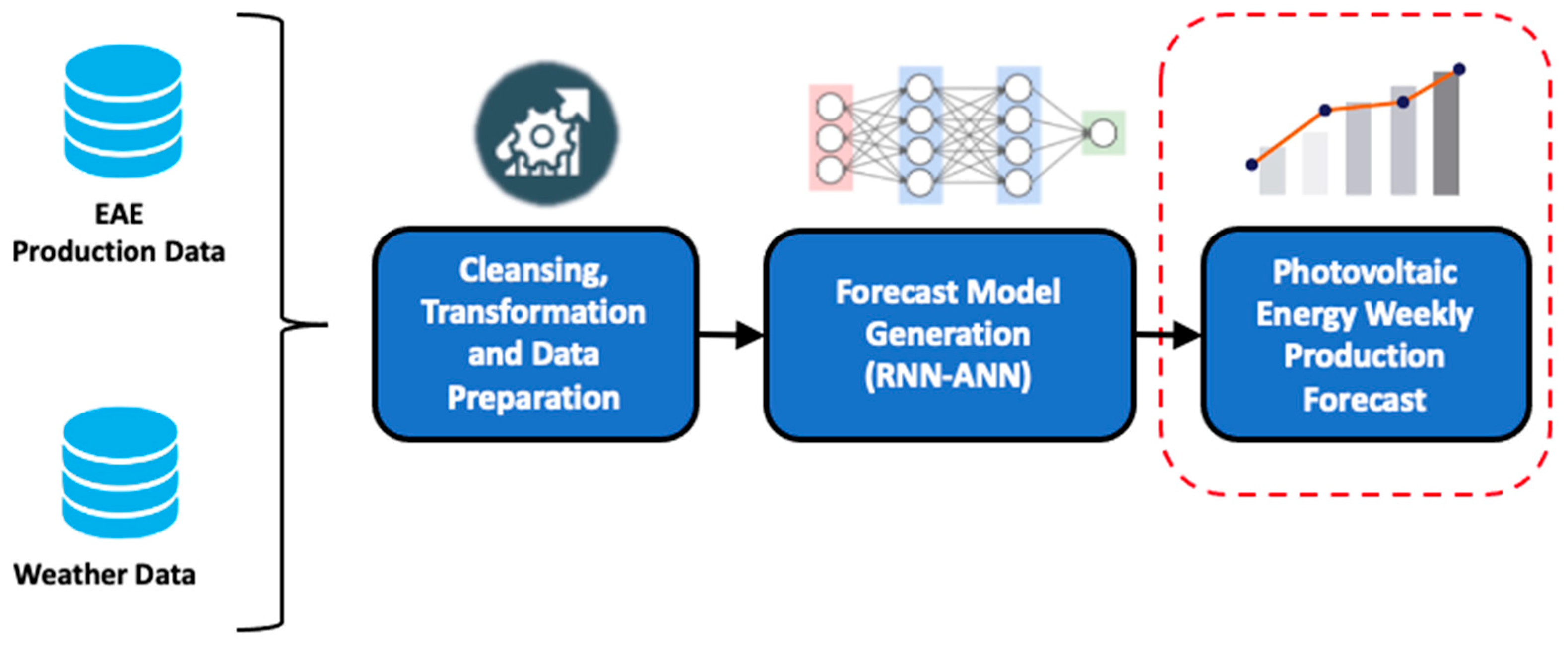
The objective of this work was to develop models that can forecast the generation of photovoltaic energy with a high level of accuracy using historical production records and climatic measurements collected during one year. Figure 1 illustrates the general work method used to achieve this objective.

Figure 1. General working method.

As shown in Figure 1, the data for this study came from two sources: one providing EAE production records and the other providing weather variables collected from weather stations installed inside the solar plant. To achieve the study’s objective, several operations were performed on the data, such as integration, exploration, cleansing, filling, and transformation. In addition, it was necessary to prepare an adequate data representation for handling time series with RNN techniques.

Subsequently, forecast models were generated using the RNN–ANN hybrid architecture designed and explained in [11]. These models were created using various hyperparameter configurations and trained, validated, and evaluated using five performance metrics. The models with the highest performance and accuracy were selected based on the evaluation metrics. A comparative analysis of the models was then carried out, and the results were interpreted.

3.3. Preliminary Analysis and Data Preparation

The dataset was stored in separate CSV files, with each file containing information for a single month of measurement. As a result, the frequency of the records varied. EAE measurements were taken hourly, while weather variables were measured every 5 min.

The daily production of EAE was recorded in kilowatt-hours (kWh). Weather variables such as compensated irradiation in watts per square meter (W/m²), ambient temperature in degrees Celsius (°C), wind speed in kilometers per hour (km/h), and wind angle in degrees (°) were also available. These data are presented together with a timeline that includes date and time.

To integrate data from both sources, an exploratory analysis was first carried out. It was observed that the values of the weather variables did not vary substantially within one hour. Therefore, the average value of each weather variable for each hour was established by aligning it with the same hourly frequency of the data in the EAE variable.

The date and time information were combined into a single column. However, a challenge arose regarding the range of values for sun radiation due to the presence of negative readings in some pyranometers when there was no solar radiation. Instead of registering zero, the pyranometers registered a negative value. To address this issue, the negative readings of sun radiation were replaced by zeros. The dataset also contained missing data in various segments, particularly in weather variables. To address this, various data filling techniques were applied depending on the characteristics of the variables.

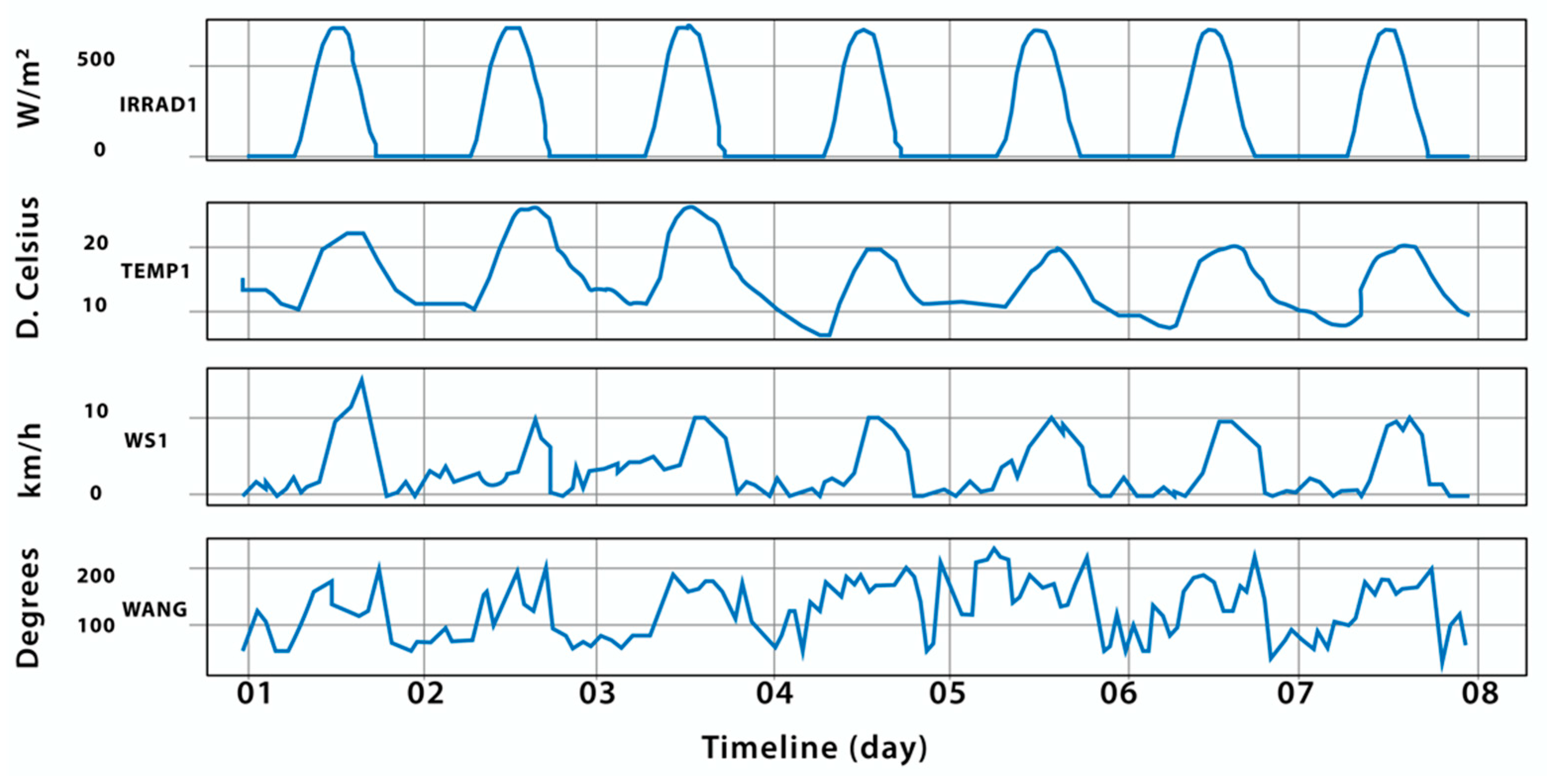
Figure 2 depicts a sample of weather variable records spanning one week. The temperature and sun radiation exhibited comparable behavior, showing a strong link. Wind speed and angle, on the other hand, followed a chaotic and unpredictable pattern. As a result, missing values for certain variables were handled differently. In particular, missing values for wind speed and angle were filled with the preceding value, because the curves of these variables indicated local patterns, and each value was strongly related to the previous one.

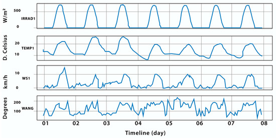
Figure 2. Exploratory sample of records in weather variables.

In the case of variable temperature and sun radiation, methods for filling in time series from different authors have been reviewed [45,46,47,48]. However, for this work, it was decided to use the technique described in [49] due to its simplicity of application and because it does not affect the performance of forecast models. This method involves completing the missing data based on the average. Each missing value was replaced by the average of the values of the seven days before or after, corresponding to the same time of day. For example, if the temperature value for 14 June at 10:25 a.m. was absent, the average of the temperature values at 10:25 a.m. of the seven days before was calculated, from 7 to 13 June. The value resulting from this calculation was used to replace the missing data. This method respects the local and daily trends of the variables. It was valid and could be carried out, as the missing data segments did not exceed 288 records. These methods were selected for their speed of execution and satisfactory results for relatively small missing segments.

On the other hand, the electrical variable EAE does not have missing values. However, it does present negative outliers in some records, which are not meaningful in this type of data. It is presumed that this anomaly can be attributed to the measuring instrument used. To solve this problem, the negative values are replaced with their absolute values, considering that the magnitude at the affected points aligns with the expected values.

Extreme values are identified in the EAE variable, and an analysis is carried out to establish a threshold limit within its range of values. Taking into account that the maximum power registered in the solar plant is approximately 9 MW, a threshold of 10 MW is defined. Because these cases are uncommon, values greater than 10 MW are replaced by the first value belonging to the 99th percentile of all records for this variable.

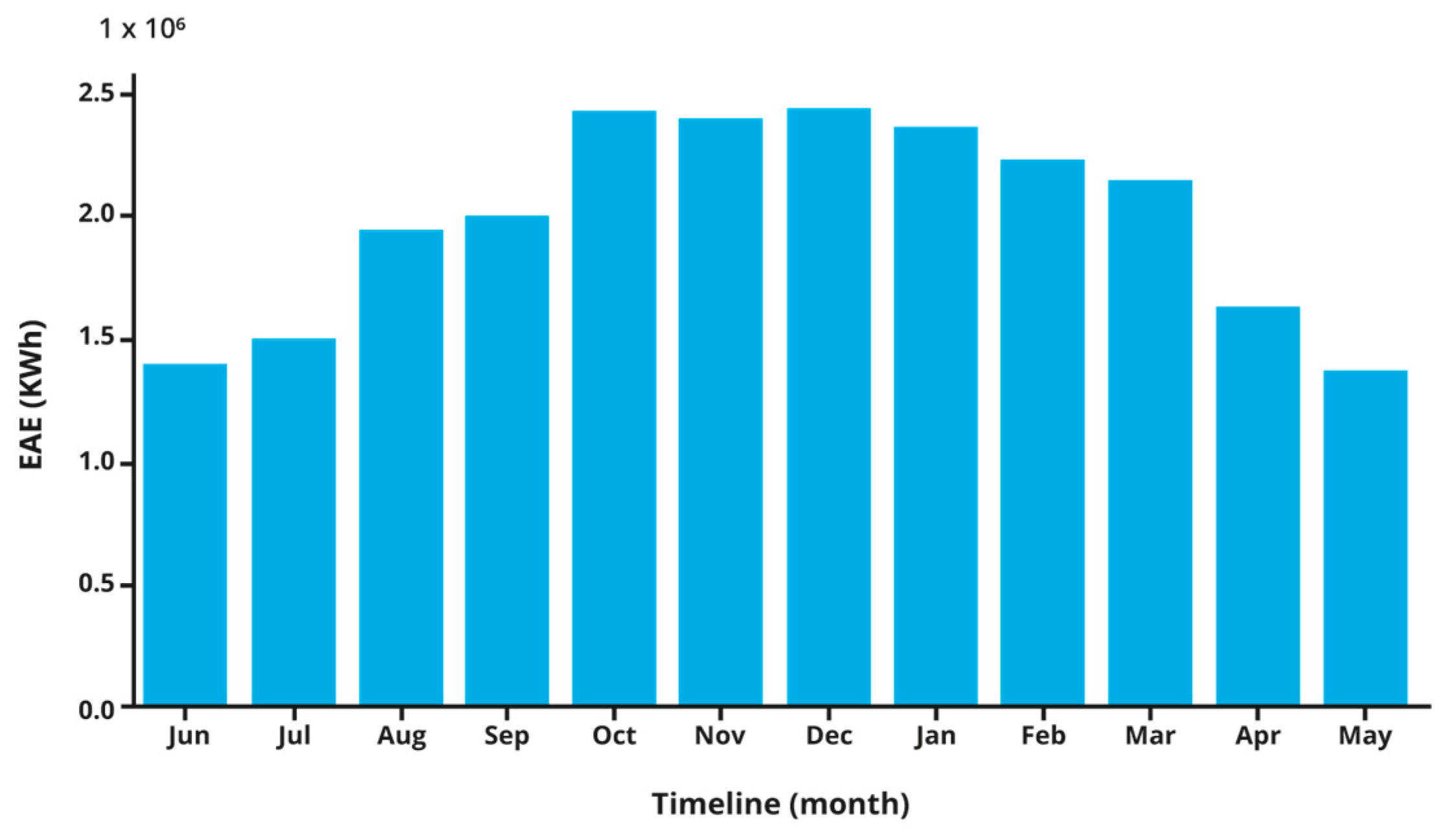
Additionally, as shown in Figure 3, the monthly generation of EAE by the solar plant during the observation period was examined. It can be seen that the months with the highest photovoltaic energy output, which run from October to March, must correlate to the spring and summer seasons in this location. In the autumn and winter seasons, the months of decreasing outputs were from April to September. This was primarily due to the sun radiation behavior at these sites, which is closely related to the EAE produced.

Figure 3. Monthly EAE production.

As mentioned above, the raw data was separated into different files per month. Therefore, a data integration task was initially performed by processing each file. Pre-processing tasks were performed for each variable. Once completed, the processed data were integrated into a single table containing all records for the work period, ordered chronologically.

3.4. Data Transformation

Once the previous data preparation has been completed, ad-hoc transformations must be carried out for appropriate use by the RNN technique. These transformations should be based on the characteristics of the technique and the model to be obtained. Both the inputs and the structure of the model must be prepared, and the dataset should be divided before moving on to the modeling process.

For this particular work, it was necessary to transform the data into a supervised structure, as RNN models require training that is defined by input and output labels. Furthermore, the research data was accompanied by a timestamp, and the research objectivewas to make time-based predictions.

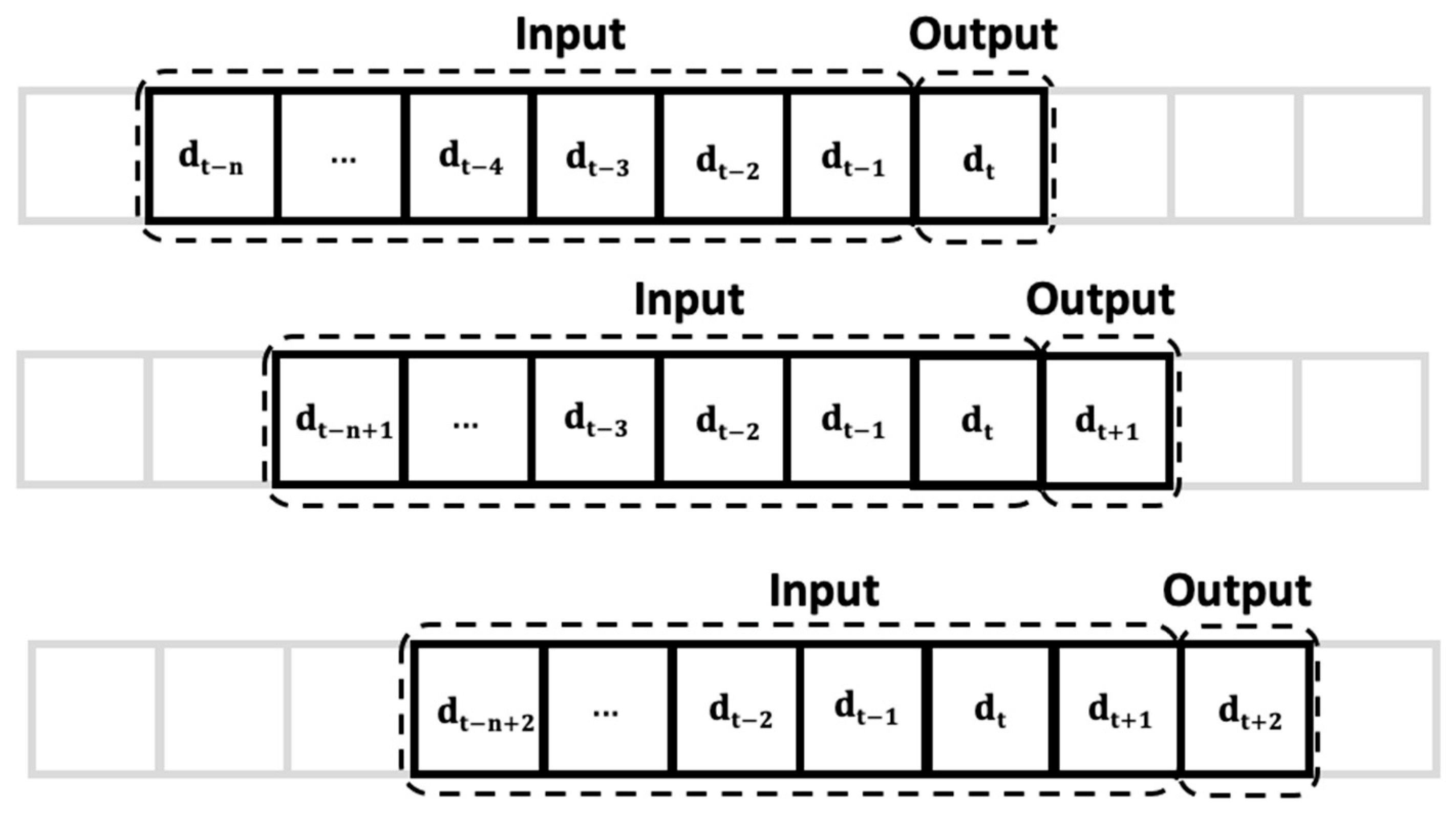
Therefore, it was decided to define the inputs of the model as time series, which means that each input is composed of a sequence of $n$ records. The models were trained, taking into account that for an output $d_t$, there is an input that covers several records from $d_{t-1}$ to $d_{t-n}$. The data were transformed based on the size of the input and output streams. This process was performed iteratively. As a result, the data were restructured into input and output pairs, as shown in Figure 4.

Figure 4. Sequence structure for time series.

It is common for such transformations to undergo multiple changes during the data analysis process, typically due to modifications to the model or during the evaluation stage. These changes often involve adjusting the sizes of the input and output sequences.

Finally, it is necessary to apply normalization to the data so that they can be re-scaled and managed within the same range, which minimizes the effect of variation or noise. One of the most commonly used types of normalization is the minimum–maximum normalization, which involves transforming each data point according to the following equation:

$$x^{\prime }=\frac{x-x_{min}}{x_{max}-x_{min}}$$

(1)

This process is carried out independently for each variable, as they each have their own range and scale. Once the model results are obtained, they must be inverted or denormalized to obtain the values in the original scale. For this work, standardization is used, since it yields better results.

3.5. Model Generation Tool

A computational tool was developed to automate the entire process, starting from data extraction and cleansing, to data preparation and transformation, as well as the generation of forecasting models with their corresponding graphs, model training and validation, and performance evaluation using various metrics. This tool provides a general framework for carrying out time series forecasting tasks and can be adapted to different scenarios and data sources.

For the development of this tool, the Python programming language was used in conjunction with the TensorFlow framework. The latter offers a comprehensive set of open-source libraries and resources to facilitate machine learning development. Additionally, the Keras API was used, which is one of the main components of TensorFlow and covers each step of the machine learning workflow.

As an input, the tool requires two files: one with the training and validation dataset and another with the configured hyperparameters. For each execution, the tool generates two output files. The first file contains the generated model and its graphs of loss, forecast, and dispersion function curves, comparing the forecast data with the actual data on the weekly production of EAE. The second file contains the results obtained for each of the metrics applied to the model.

This method of building the computational tool provides flexibility and generalization of the inputs. For example, it allows for the reconfiguration of hyperparameters to obtain a different model, changing the data set, or both inputs simultaneously.

4. RNN–ANN Models

This work is based on a hybrid RNN–ANN architecture that was designed in the previous section of this study and thoroughly described in [11]. The RNN–ANN architecture is made up of two hidden layers: the first uses recurrent neurons with LSTM or GRU units, and the second layer is composed of shallow neurons organized in an MLP structure. The significance of this architecture lies in its pre-existing and tested structure for generating forecast models of photovoltaic energy production using a single input variable. However, in this implementation, it has been configured to accommodate multiple variables as input for the models.

The contributions of this work build upon the previous part of this research by focusing on the validation of the RNN–ANN hybrid architecture through the generation of models that incorporate multiple input variables, as well as the exploration of various hyperparameter configurations. The variables used as inputs for the models included historical EAE records, as well as available weather variables such as sun radiation, temperature, and wind speed. These data corresponded to records collected throughout one year. In addition, the hyperparameters of the internal components of the model, such as the activation function and the loss function, were also fitted.

Different controlled experiments are conducted to obtain the models with the best performance, evaluated using a combination of appropriate metrics. Two types of models are generated for this purpose:

• Models with EAE records and weather variable measurements as input variables, accompanied by a timeline;
• Models that solely use weather variables as input variables, accompanied by a timeline.

To improve the performance of a model, it is important to configure several hyperparameters based on its features. For example, the number of neurons in the hidden layers can vary depending on whether the model has a single input variable or multiple input variables. Similarly, the number of batches and the activation function may need to be adjusted based on the number and type of input variables.

4.1. Models with EAE and Weather Variable Inputs

When configuring models, all necessary hyperparameters are considered, including the size of the input and output sequences, the division of the data set for training and validation, the type and number of recurring neurons in the hidden layers, and the batch size, activation functions, loss function, learning rate, optimizer, and performance metrics. Table 2 presents the hyperparameters used in the preliminary or test models. This aids in the identification and selection of optimal values for the final model configuration in this study. These adjustments were made through a series of experiments.

Table 2. Configuration of the models with all the variables.

Hyperparameters	Configuration
Number of recurrent neurons	100
Activation function	Relu
Loss function	Huber
Optimizer	Adam
Input sequence size	72
Dataset split	80% training, 20% testing

It is important to highlight that in the preliminary tests of the models using the entire provided dataset, undesired overtraining phenomena were observed when a training process of 100 epochs was defined. Therefore, after several tests, the number of epochs was set to 20, as the models were able to stabilize with this number.

Considering the exploratory analysis of the meteorological variables described in Section 3.3 and depicted in Figure 2, the decision was made to exclude the wind angle variable (WANG) from the models. This is attributed to its chaotic behavior and the absence of a direct relationship with the sun radiation and temperature variables. Thus, for model generation, only the following variables will be utilized: EAE, IRRAD, TEMP, WS, and Timestamp (date and time).

Starting from this base model, new experiments were carried out using different configurations for each hyperparameter until the results were within a good level of forecasting and acceptable ranges in the evaluation metrics were achieved. Based on the results obtained for each hyperparameter, models with the best performance were pre-selected, as shown in Table 3. Regarding the hyperparameter number of inputs, two types of models were selected: those with three input variables (EAE, IRRAD, and TEMP), and those with four input variables (EAE, IRRAD, TEMP, and WS), which were always accompanied by a timestamp. For all these models, 20 recurrent neurons and a dataset split of 90% for training and 10% for testing were used.

Table 3. Pre-selected models.

Models	Activation Function	Loss Function	Optimizer	Input Sequence Size	Number of Inputs
Model 1	Relu	MSE	RMSprop	72	3
Model 2	Relu	LogCosh	RMSprop	72	3
Model 3	LeakyReLU	MSE	RMSprop	72	3
Model 4	LeakyReLU	MSE	RMSprop	24	3
Model 5	LeakyReLU	MSE	RMSprop	24	4
Model 6	LeakyReLU	MSE	Adam	24	4

The results of the metrics for these models are presented in Table 4, where the best performance is compared to the other previously tested models.

Table 4. Metric results of preselected models.

Models	Correlation Coefficient	Determination Coefficient	MSE	MAE	RMSE
Model 1	0.962988	0.927196	0.045359	0.107983	0.212976
Model 2	0.963756	0.927210	0.043488	0.103623	0.208519
Model 3	0.962180	0.924341	0.040797	0.094496	0.201982
Model 4	0.965271	0.931373	0.039147	0.090114	0.197855
Model 5	0.964508	0.930250	0.040490	0.092352	0.201220
Model 6	0.960609	0.921630	0.043614	0.100860	0.208840

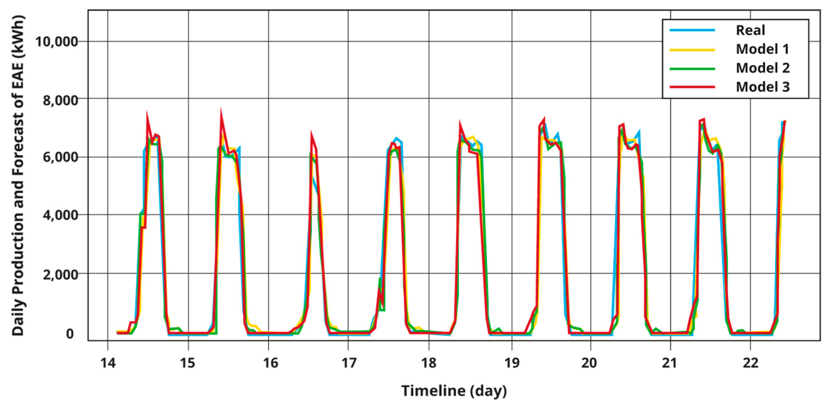
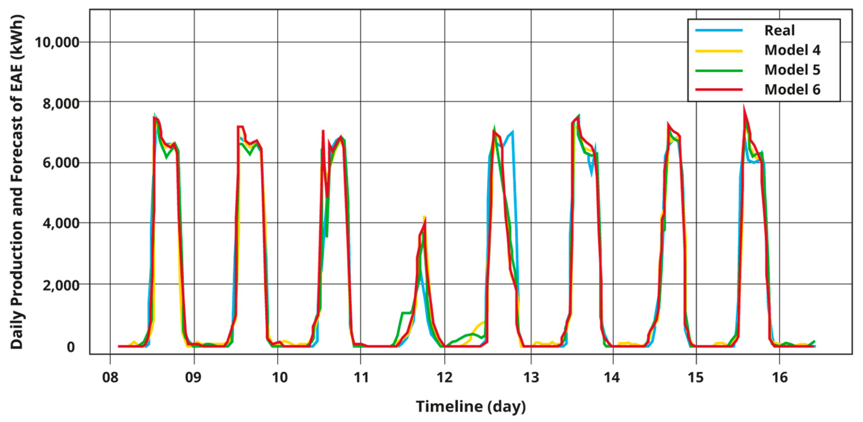
Figure 5 and Figure 6 graphically present the results obtained from running the six preselected models with the indicated hyperparameter configurations. Models 1 and 4 stand out for their level of forecasting accuracy, closely resembling the actual curve of the EAE production data. However, Model 4 achieved the best results in all metrics. It exhibited the highest correlation coefficient (0.965271) and determination (0.931373), as well as the lowest errors (MSE = 0.039147, MAE = 0.090114, RMSE = 0.197855). This allowed us to deduce that the RNN–ANN hybrid architecture, with a smaller input sequence, achieves better performance in the models it generates.

Figure 5. Daily forecast of pre-selected models with an input sequence size of 72.

Figure 6. Daily forecast of pre-selected models with an input sequence size of 24.

In general, a reliable approximation to the actual production of EAE was noted, with the main failures occurring on very isolated days with irregular weather phenomena. Furthermore, it was observed that Model 6, despite not yielding the best metrics results, was the most stable and presented fewer disturbances during hours of absent sun due to the Adam optimizer used to implement this model.

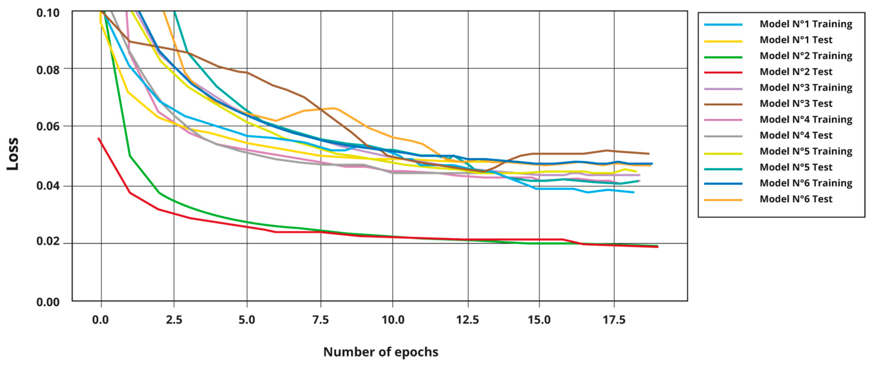
The loss function of these models is shown in Figure 7, where an appropriate behavior can be observed for each model, as their training and testing curves converge in most cases, despite the small number of epochs used in training. Model 2 stands out due to its use of a different loss function, and the models that received an input sequence of 72 elements tended to undergo slight changes during the training process.

Figure 7. Loss curve graphs for pre-selected models.

4.2. Models with Only Weather Input Variables

For this type of model, experiments were also conducted to analyze which input variables were most appropriate. A base configuration was established to generate these models, with the main difference being the size of the input sequence. One set had a size of 72 elements, and the other had a size of 24 elements. A combination of input variables was also used. Table 5 presents the configuration of the hyperparameters for the base model.

Table 5. Model setup with only weather variables.

Hyperparameters	Configuration
Number of recurrent neurons	20
Activation function	Relu
Loss function	LogCosh
Optimizer	RMSprop
Input sequence size	72/24
Data set split	90% training, 10% testing

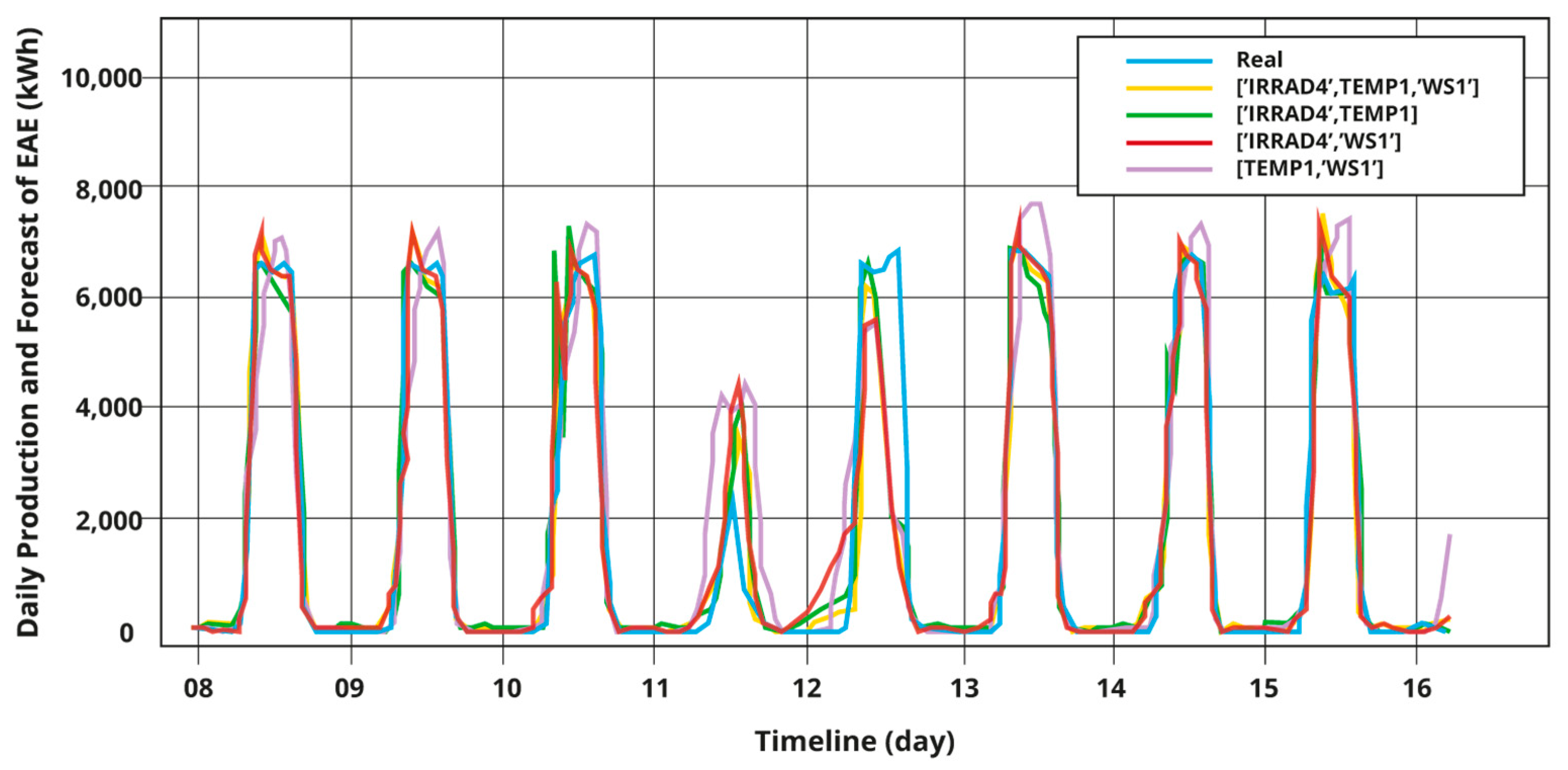
Table 6 and Table 7 show the results of the metrics achieved by the models with input sequence sizes of 72 and 24 elements, respectively, for different combinations of weather variables. In both cases, it was confirmed that the best combination of input variables was sun radiation and temperature, which achieved the best results in performance metrics such as the correlation coefficient and determination coefficient.

Table 6. Results with a sequence size of 72 in the input.

Inputs	Correlation Coefficient	Determination Coefficient	MSE	MAE	RMSE
IRRAD, TEMP, WS	0.945908	0.888276	0.064001	0.114441	0.252984
IRRAD, TEMP	0.952505	0.906126	0.063654	0.121831	0.252297
IRRAD, WS	0.941199	0.868623	0.070948	0.127403	0.266360
TEMP, WS	0.893265	0.795375	0.129587	0.188416	0.359982

Table 7. Results with a sequence size of 24 in the input.

Inputs	Correlation Coefficient	Determination Coefficient	MSE	MAE	RMSE
IRRAD, TEMP, WS	0.950260	0.901154	0.061535	0.110532	0.248053
IRRAD, TEMP	0.951835	0.904166	0.060122	0.108557	0.245197
IRRAD, WS	0.940340	0.882897	0.065238	0.115602	0.255417
TEMP, WS	0.900719	0.806981	0.129571	0.186893	0.359959

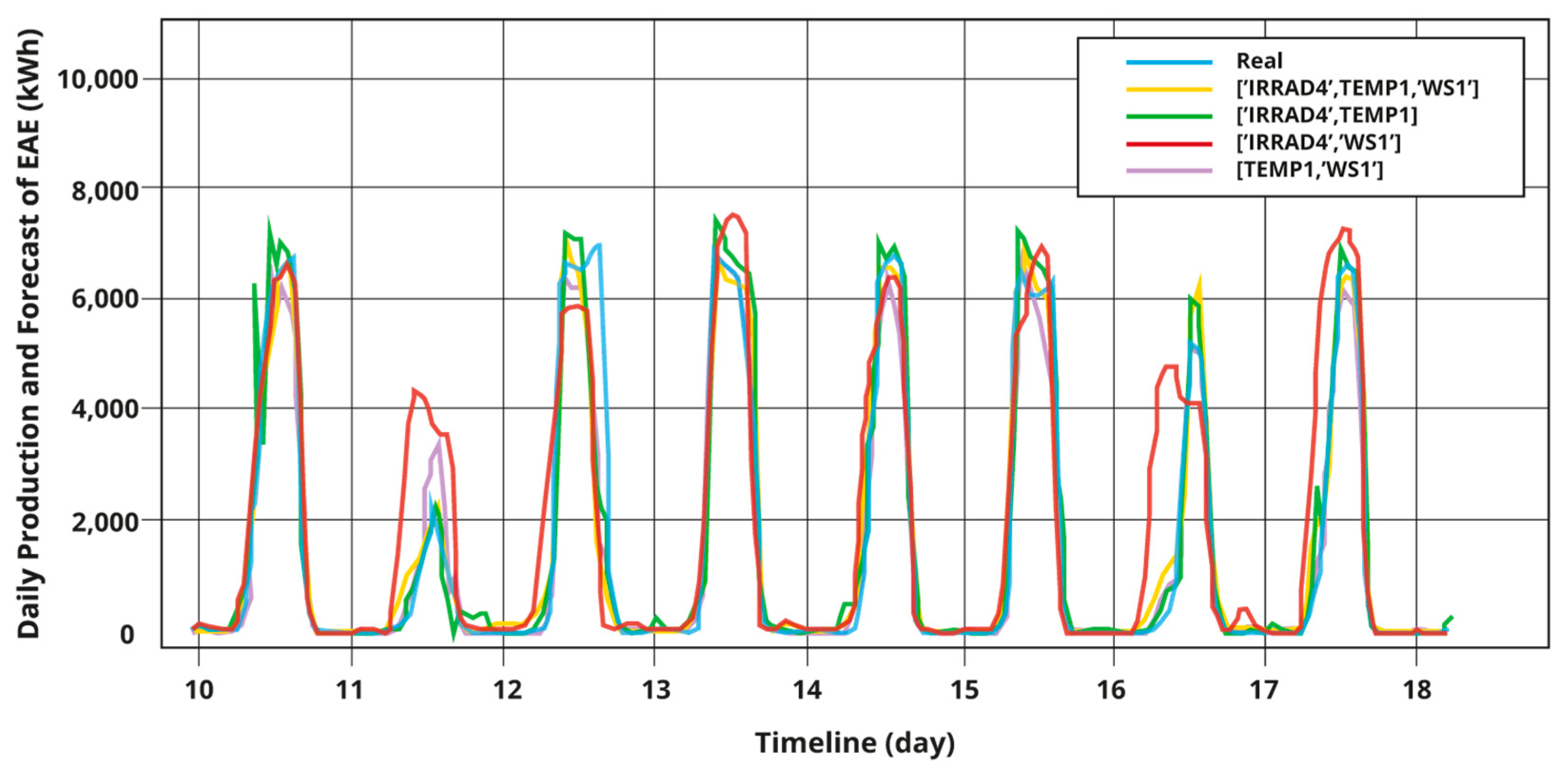
Figure 8 and Figure 9 display the daily forecasts obtained by these models for input sequence sizes of 72 and 24 elements, respectively. These graphs confirm that the combination of radiation and temperature variables provided a higher level of forecast accuracy.

Figure 8. Daily forecast of models with input sequence sizes of 72.

Figure 9. Daily forecast of models with input sequence sizes of 24.

Since these models only used weather variables, they did not achieve better metric results than the first type of model. However, they still provided a forecast that closely matched the real data.

5. Results and Discussion

It was possible to develop models to accurately forecast the weekly production of photovoltaic energy based on historical records of EAE and meteorological measurements, both accompanied by a timeline. The different related works analyzed in Section 2 were used as a reference. Specifically, the studies carried out in [25,26] were discussed due to their relevance to this research.

The main achievement of this work was to validate the RNN–ANN architecture for generating forecast models with multiple input variables. These models demonstrated high accuracy in forecasting photovoltaic energy generation using EAE production records and weather measurements collected over the course of a year.

There are hyperparameters that must be properly configured for the RNN–ANN forecast model. Many preliminary experiments were carried out from a base model with the goal of determining the appropriate hyperparameter configurations to generate the final forecast models. The experimental part of the work focused on generating two types of models based on the input variables.

The first type of model utilized the EAE variable, along with the IRRAD, TEMP, and WS weather variables. It used 20 recurrent neurons and divided the dataset into 90% for training and 10% for validation. The configurations are shown in Table 3. Six models of this type were obtained, which yielded good results in the evaluation metrics applied, as shown in Table 4.

For the second type of model, only weather variables were used, and eight models were obtained with different combinations of these variables, differentiated only by the input sequence size. The hyperparameters used for these models included 20 recurrent neurons and a 90% training and 10% validation data set split, which are shown in Table 5, Table 6 and Table 7.

The models of the second type yielded lower values in their metrics compared to the models of the first type, which can be observed by comparing Table 4, Table 6 and Table 7. This result was expected, as the absence of the EAE variable as input made the model more prone to issuing output distortions. However, the obtained models could forecast photovoltaic energy generation in solar plants using conventional weather forecasts.

Table 8 shows the metrics results for the models with the best performance in each type. Model 4 excelled in all metrics for the first type, while the model that forecasted from the combination of solar radiation and temperature variables obtained the best results for the second type.

Table 8. Selected models for each type.

Selected Models	Correlation Coefficient	Determination Coefficient	MSE	MAE	RMSE
Model 4 (of Table 4)	0.965271	0.931373	0.039147	0.090114	0.197855
Model with IRRAD and TEMP (of Table 7)	0.951835	0.904166	0.060122	0.108557	0.245197

Although both models were able to forecast the weekly production of photovoltaic energy, they presented small errors and differences in some observed intervals. However, when comparing the results with those obtained in the works most closely related to this research (Che et al. [25] and Sharadga et al. [26]), it was found that Model 4 improved an average of 60% in the RMSE metric shared by both works, while the model of the second type improved in the RMSE metric by 45%. These results can still be improved upon by increasing the volume of data and extending the forecast period.

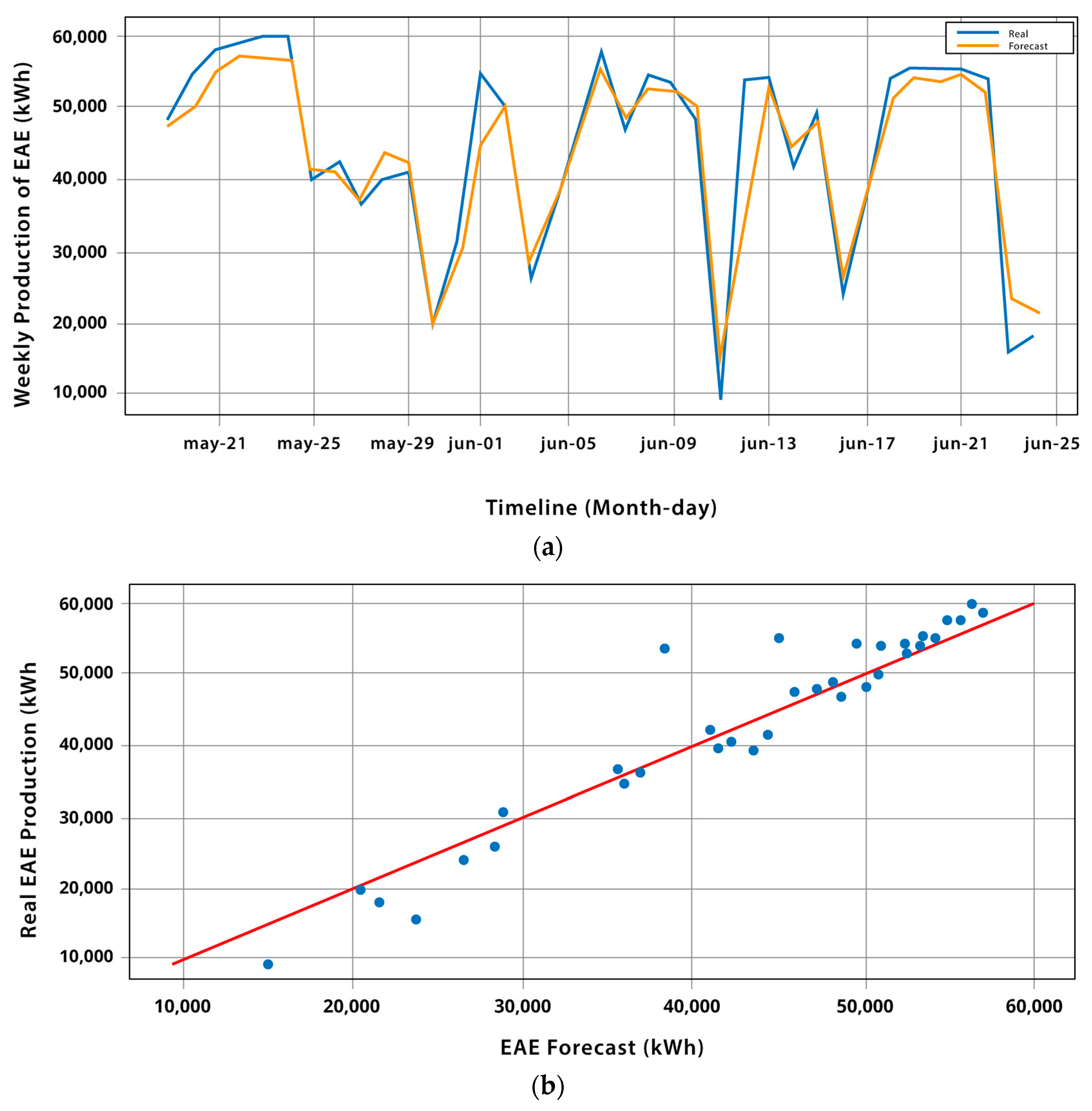
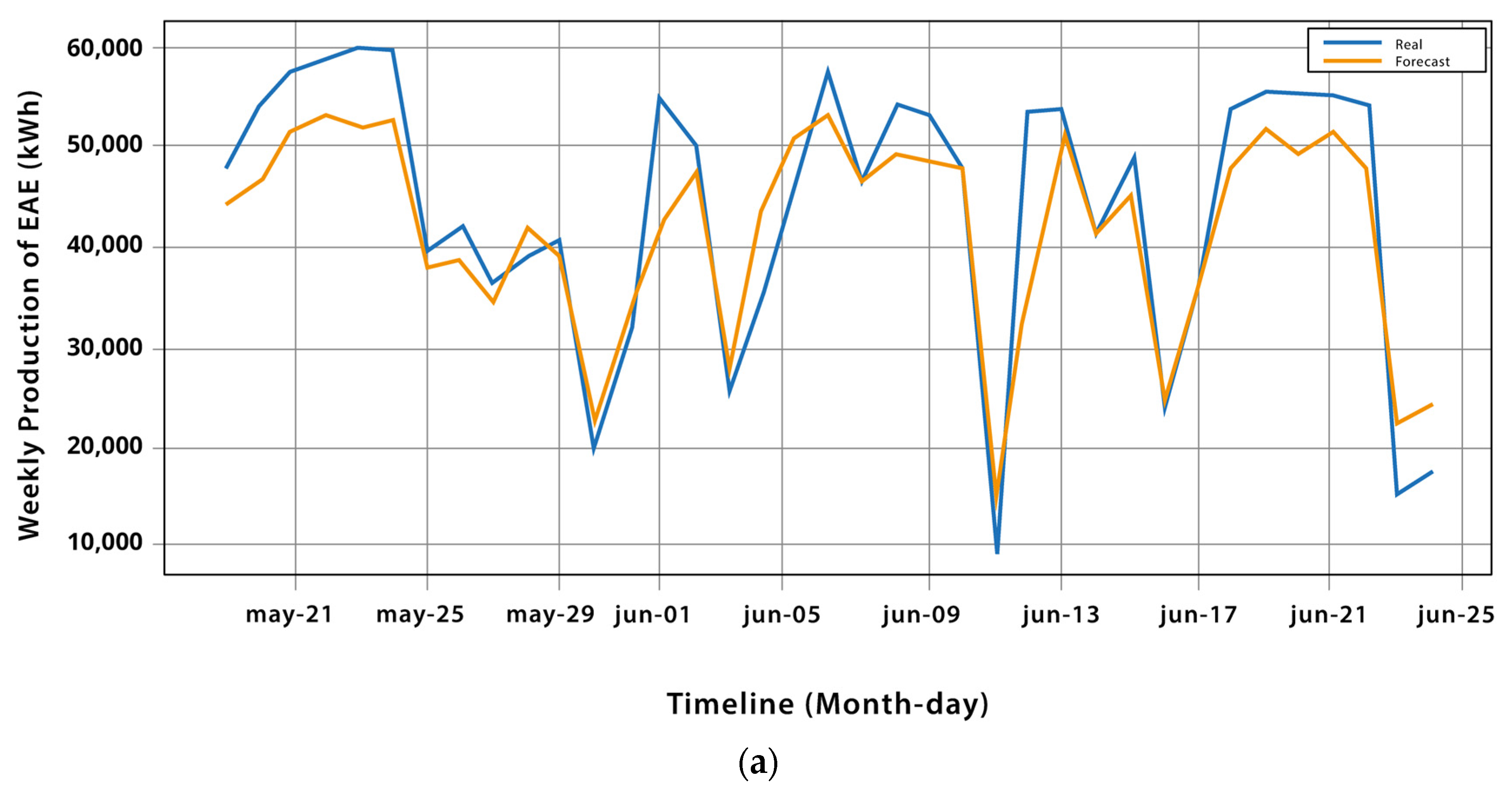
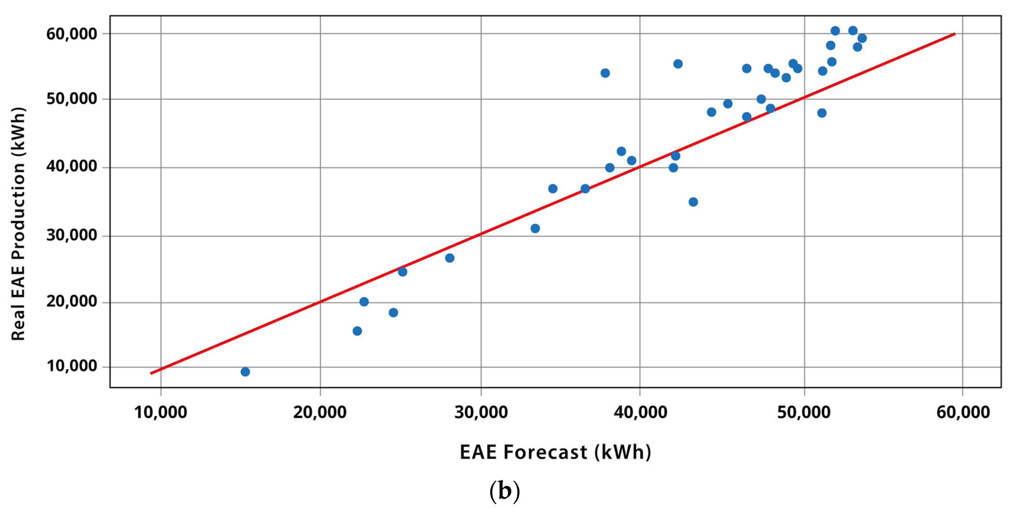
Figure 10 and Figure 11 illustrate select results of the chosen models, as indicated in Table 8. In each figure, Graph (a) displays the weekly forecast for the months of May and June, while Graph (b) presents a scatterplot comparing the predicted values to the actual values of the solar plant’s weekly EAE production. In the scatterplots, the red line represents the linear trend of EAE production in both the actual and forecasted data. The blue dots represent the spread of the forecasted data relative to their corresponding real EAE production data.

Figure 10. Model with EAE and weather variables. (a) Weekly forecast; (b) dispersion between forecast and real values.

Figure 11. Model with only weather variables. (a) Weekly forecast; (b) dispersion between forecast and real values.

When Figure 10a and Figure 11a are compared, it is clear that both models are capable of accurately estimating weekly photovoltaic energy production while maintaining a behavior similar to the real data curve. However, the model that combines the EAE and weather variables (model 4 in Table 4) showed higher precision and a better fit to the real data curve across the entire observed time.

Similar patterns can be observed in the scatter diagrams of Figure 10b and Figure 11b. Although both models showed a clear correlation between the forecast and real data, Model 4 excelled with the EAE and meteorological variables as input, as it had less data dispersion points with regard to the real values. This was quantitatively confirmed by the correlation coefficients (0.965271) and determination (0.931373) shown in Table 8 compared to the same metrics obtained by the model that only used meteorological variables (correlation coefficient: 0.951835, determination: 0.904166). In addition, Model 4 surpassed the model of the second type in the other metrics by approximately 35% in the MSE, 10% in the MAE, and 20% in the RMSE.

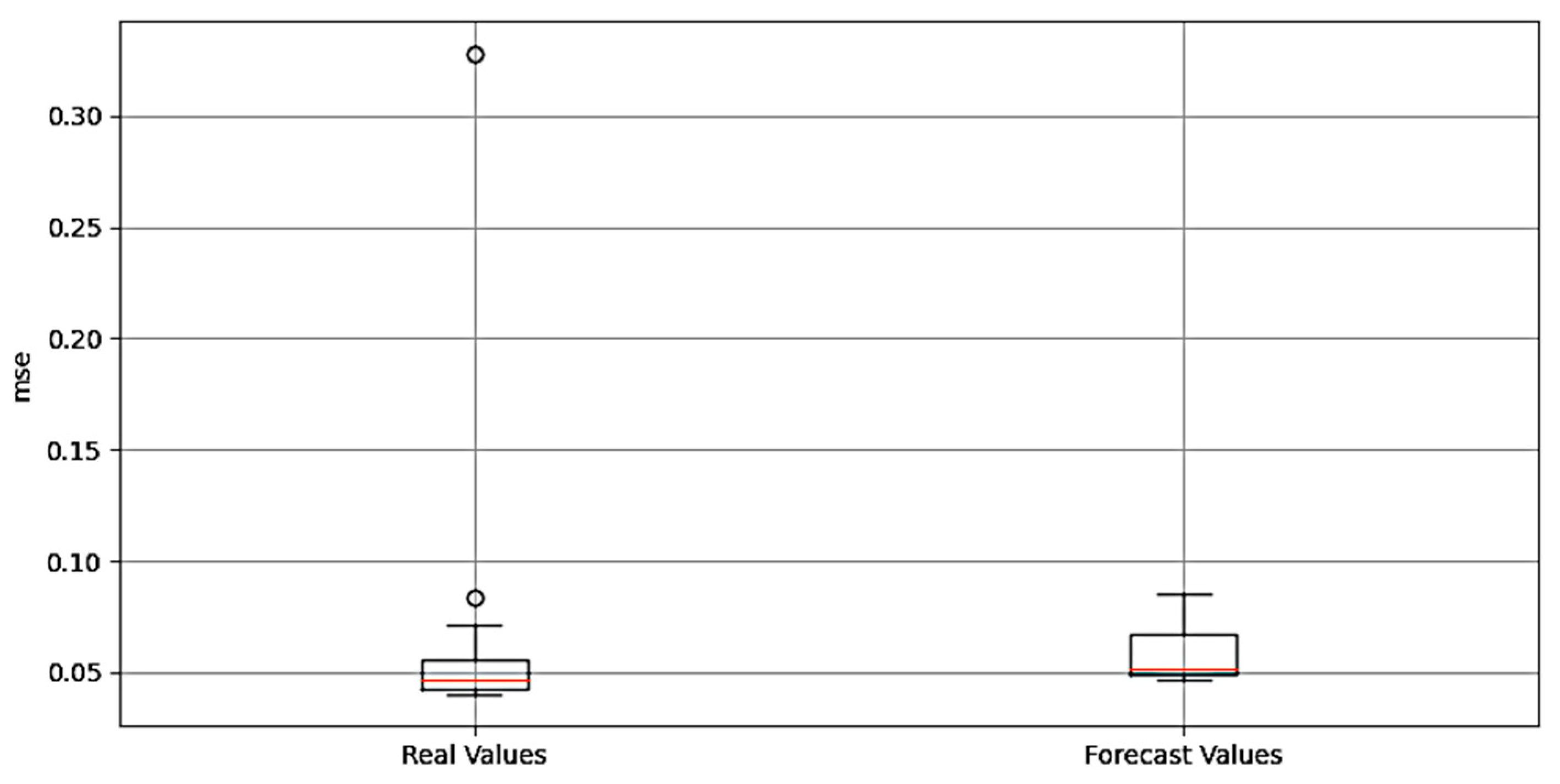
To complement this analysis, Figure 12 presents a visual representation of the forecast errors of Model 4, which was selected as the best model in this study. The boxplot shows the distribution of errors for the training and test sets using the MSE metric. These errors are acceptable and support the reliability of the quantitative analysis performed. In this graph, the circles that appear represent outliers. The red line represents the third quartile, which means that 75% of the error values are less than or equal to the value at the top of the box.

Figure 12. Distribution of Model 4 forecast errors observed using the MSE metric.

Overall, it can be concluded that for weekly analysis, the models that incorporated the EAE variable provided better forecast results compared to the models that only used meteorological variables as inputs. This suggests that the EAE variable is a relevant factor to consider when predicting the production of photovoltaic energy.

6. Conclusions

The forecast models are useful for solar plants and their operators, allowing efficient planning to balance the generation and consumption of photovoltaic energy. Improving the accuracy of these models is essential to obtain more reliable estimates of energy production, which can be integrated into existing electrical systems. In this study, it was possible to confirm and validate the previously described RNN–ANN hybrid architecture described in [11]. This approach generates forecast models of the weekly production of photovoltaic energy in a solar plant with a high degree of accuracy using multiple input variables. Two types of models were developed: one that uses EAE records and climate variables, and another that uses only climate variables. Both types of models achieved good accuracy in forecasting weekly energy production. Model 4 of the first type obtained the best results across all of the applied metrics (RMSE = 0.19, MSE = 0.03, MAE = 0.09, correlation coefficient = 0.96, and determination coefficient = 0.93). Although the selected model of the second type presented a lower precision in some metrics (RMSE = 0.24, MSE = 0.06, MAE = 0.10, correlation coefficient = 0.95, and determination coefficient = 0.90), it still showed a positive performance for making predictions. Compared with results of works directly related to this research ([25,26]), Model 4 showed improvements of 60% in the RMSE metric shared by both works, while the model of the second type exceeded an average of 45%. This work also stands out for the use of a large dataset (more than 100,000 records) for model training and validation, which contributed to its good level of precision. In addition, a computational tool was developed for the implementation of the models and experiments, which stands out for its simplicity and flexibility in the generation of different forecast models. Due to the generality of this tool, it can be applied to other contexts such as wind energy forecasting or others, adjusting the input data and hyperparameters according to the transformations described in Section 3.4.

As a future work, the architecture, performance, and accuracy of the models can be improved. This can be done by generating new models with different configurations and RNN structures using various combinations of hyperparameters. The data set for training and validation can also be increased by incorporating additional records. Another interesting line of research would be to integrate physical aspects, such as the internal composition of the photovoltaic modules or the temperature generated by sun radiation in these components. Finally, the application of this approach to other sources of renewable energy can be explored.

References

- International Energy Agency. Trends in Photovoltaic Applications 2018; Report publisher by IEA PVPS T1-34: Paris, France, 2018; Volume 23, ISBN 978-3-906042-79-4. [Google Scholar]
- Arshian Sharif, A.; Saeed, M.; Ferdous, M.; Sohag, K. Role of solar energy in reducing ecological footprints: An empirical analysis. J. Clean. Prod. 2021, 292, 126028. [Google Scholar] [CrossRef]
- Schloss, M.J. Cambio climático y Energía: ¿Quo vadis?, Encuentros multidisciplinares: Energía, Medio Ambiente y Avances Científicos; Nº 62; Editorial Dialnet de la Universidad de la Rioja: La Rioja, España, 2019; Volume 21, ISSN 1139-9325. [Google Scholar]
- Maleki, A.; Ahmadi, A.; Venkatesan, S. Optimal design and analysis of solar photovoltaic systems to reduce carbon footprint. Renew. Energy 2019, 141, 76–87. [Google Scholar] [CrossRef]
- Boer, S.; Steinberger-Wilckens, R.; Buchholz, D.; Meissner, D.; Schebek, L. Environmental impact and economic analysis of an integrated photovoltaic-hydrogen system for residential applications. Appl. Energy 2020, 276, 115349. [Google Scholar]
- Iheanetu, K.J. Solar Photovoltaic Power Forecasting: A Review. Sustainability 2022, 14, 17005. [Google Scholar] [CrossRef]
- Yesilbudak, M.; Çolak, M.; Bayindir, R. A review of data mining and solar power prediction. In Proceedings of the 2016 IEEE International Conference on Renewable Energy Research and Applications (ICRERA), Birmingham, UK, 20–23 November 2016; pp. 1117–1121. [Google Scholar]
- Berzal, F. Redes Neuronales & Deep Learning; Editorial Universidad de Granada: Granada, España, 2018; ISBN-10 1-7313-1433-7, ISBN-13 978-1-7313-1433-8. [Google Scholar]
- Kukreja, H.; Bharath, N.; Siddesh, C.; Kuldeep, S. An Introduction to Artificial Neural Network. Int. J. Adv. Res. Innov. Ideas Educ. 2016, 1, 27–30. [Google Scholar]
- Nwankpa, C.; Ijomah, W.; Gachagan, A.; Marshall, S. Activation Functions: Comparison of Trends in Practice and Research for Deep Learning. arXiv 2018, arXiv:1811.03378. [Google Scholar]
- Castillo-Rojas, W.; Bekios-Calfa, J.; Hernández, C. Daily Prediction Model of Photovoltaic Power Generation Using a Hybrid Architecture of Recurrent Neural Networks and Shallow Neural Networks. Int. J. Photoenergy 2023, 2023, 2592405. [Google Scholar] [CrossRef]
- Maciel, J.N.; Wentz, V.H.; Ledesma, J.J.G.; Junior, O.H.A. Analysis of Artificial Neural Networks for Forecasting Photovoltaic Energy Generation with Solar Irradiance. Braz. Arch. Biol. Technol. 2021, 64 no.spe, e21210131. [Google Scholar] [CrossRef]
- Rodríguez, F.; Azcárate, I.; Vadillo, J.; Galarza, A. Forecasting intra-hour solar photovoltaic energy by assembling wavelet-based time-frequency analysis with deep learning neural networks. Int. J. Electr. Power Energy Syst. 2021, 137, 107777. [Google Scholar] [CrossRef]
- Carrera, B.; Sim, M.; Jung, J. PVHybNet: A hybrid framework for predicting photovoltaic power generation using both weather forecast and observation data. IET Renew. Power Gener. 2020, 14, 2192–2201. [Google Scholar] [CrossRef]
- Rosato, A.; Araneo, R.; Andreotti, A.; Panella, M. Predictive Analysis of Photovoltaic Power Generation Using Deep Learning. In Proceedings of the IEEE International Conference on Environment and Electrical Engineering and IEEE Industrial and Commercial Power Systems Europe (EEEIC/I&CPS EUROPE), Genova, Italy, 10–14 June 2019. [Google Scholar]
- Yu, Y.; Cao, J.; Zhu, J. An LSTM Short-Term Solar Irradiance Forecasting Under Complicated Weather Conditions. IEEE Access 2019, 7, 145651–145666. [Google Scholar] [CrossRef]
- Hui, L.; Ren, Z.; Yan, X.; Li, W.; Hu, B. A Multi-Data Driven Hybrid Learning Method for Weekly Photovoltaic Power Scenario Forecast. IEEE Trans. Sustain. Energy 2022, 13, 91–100. [Google Scholar] [CrossRef]
- Xu, D.; Shao, H.; Deng, X.; Wang, X. The Hidden-Layers Topology Analysis of Deep Learning Models in Survey for Forecasting and Generation of theWind Power and Photovoltaic Energy. Comput. Model. Eng. Sci. 2022, 131, 567–597. [Google Scholar] [CrossRef]
- Nkambule, M.S.; Hasan, A.N.; Ali, A.; Hong, J.; Geem, Z.W. Comprehensive Evaluation of Machine Learning MPPT Algorithms for a PV System Under Different Weather Conditions. J. Electr. Eng. Technol. 2020, 16, 411–427. [Google Scholar] [CrossRef]
- Wang, F.; Yu, Y.; Zhang, Z.; Li, J.; Zhen, Z.; Li, K. Wavelet Decomposition and Convolutional LSTM Networks Based Improved Deep Learning Model for Solar Irradiance Forecasting. Appl. Sci. 2018, 8, 1286. [Google Scholar] [CrossRef]
- AlKandari, M.; Ahmad, I. Solar power generation forecasting using ensemble approach based on deep learning and statistical methods. Appl. Comput. Inform. 2019; ahead-of-print. [Google Scholar] [CrossRef]
- Sharma, E. Energy forecasting based on predictive data mining techniques in smart energy grids. Energy Inform. 2018, 1, 44. [Google Scholar] [CrossRef]
- Harrou, F.; Kadri, F.; Sun, Y. Forecasting of Photovoltaic Solar Power Production Using LSTM Approach. In Advanced Statistical Modeling, Forecasting, and Fault Detection in Renewable Energy Systems; IntechOpen: London, UK, 2020. [Google Scholar] [CrossRef]
- De, V.; Teo, T.; Woo, W.; Logenthiran, T. Photovoltaic power forecasting using LSTM on limited dataset. In Proceedings of the 2018 IEEE Innovative Smart Grid Technologies-Asia (ISGT Asia), Singapore, 22–25 May 2018; pp. 710–715. [Google Scholar]
- Chen, B.; Lin, P.; Lai, Y.; Cheng, S.; Chen, Z.; Wu, L. Very-Short-Term Power Prediction for PV Power Plants Using a Simple and Effective RCC-LSTM Model Based on Short Term Multivariate Historical Datasets. Electronics 2020, 9, 289. [Google Scholar] [CrossRef]
- Sharadga, H.; Hajimirza, S.; Balog, R.S. Time series forecasting of solar power generation for large-scale photovoltaic plants. Renew. Energy 2019, 150, 797–807. [Google Scholar] [CrossRef]
- Rajagukguk, R.A.; Ramadhan, R.A.; Lee, H.-J. A Review on Deep Learning Models for Forecasting Time Series Data of Solar Irradiance and Photovoltaic Power. Energies 2020, 13, 6623. [Google Scholar] [CrossRef]
- Seera, M.; Jun, C.; Chong, K.; Peng, C. Performance analyses of various commercial photovoltaic modules based on local spectral irradiances in Malaysia using genetic algorithm. Energy J. 2021, 223, 120009. [Google Scholar] [CrossRef]
- Chong, K.-K.; Khlyabich, P.P.; Hong, K.-J.; Reyes-Martinez, M.; Rand, B.P.; Loo, Y.-L. Comprehensive method for analyzing the power conversion efficiency of organic solar cells under different spectral irradiances considering both photonic and electrical characteristics. Appl. Energy 2016, 180, 516–523. [Google Scholar] [CrossRef]
- Jaber, M.; Hamid, A.S.A.; Sopian, K.; Fazlizan, A.; Ibrahim, A. Prediction Model for the Performance of Different PV Modules Using Artificial Neural Networks. Appl. Sci. 2022, 12, 3349. [Google Scholar] [CrossRef]
- Diouf, M.C.; Faye, M.; Thiam, A.; Ndiaye, A.; Sambou, V. Modeling of the Photovoltaic Module Operating Temperature for Various Weather Conditions in the Tropical Region. Fluid Dyn. Mater. Process. 2022, 18, 1275–1284. [Google Scholar] [CrossRef]
- Bevilacqua, P.; Perrella, S.; Bruno, R.; Arcuri, N. An accurate thermal model for the PV electric generation prediction: Long-term validation in different climatic conditions. Renew. Energy 2020, 163, 1092–1112. [Google Scholar] [CrossRef]
- Zhang, S.; Wang, J.; Liu, H.; Tong, J.; Sun, Z. Prediction of energy photovoltaic power generation based on artificial intelligence algorithm. Neural Comput. Appl. 2020, 33, 821–835. [Google Scholar] [CrossRef]
- He, B.; Ma, R.; Zhang, W.; Zhu, J.; Zhang, X. An Improved Generating Energy Prediction Method Based on Bi-LSTM and Attention Mechanism. Electronics 2022, 11, 1885. [Google Scholar] [CrossRef]
- Chen, H.; Chang, X. Photovoltaic power prediction of LSTM model based on Pearson feature selection. Energy Rep. 2021, 7, 1047–1054. [Google Scholar] [CrossRef]
- Konstantinou, M.; Peratikou, S.; Charalambides, A.G. Solar Photovoltaic Forecasting of Power Output Using LSTM Networks. Atmosphere 2021, 12, 124. [Google Scholar] [CrossRef]
- Niccolai, A.; Dolara, A.; Ogliari, E. Hybrid PV Power Forecasting Methods: A Comparison of Different Approaches. Energies 2021, 14, 451. [Google Scholar] [CrossRef]
- Hochreiter, S.; Schmidhuber, J. Long Short-Term Memory. Neural Comput. 1997, 9, 1735–1780. [Google Scholar] [CrossRef] [PubMed]
- Schuster, M.; Paliwal, K.K. Bidirectional recurrent neural networks. IEEE Trans. Signal Process. 1997, 45, 2673–2681. [Google Scholar] [CrossRef]
- Chang, S.; Zhang, Y.; Han, W.; Yu, M.; Guo, X.; Tan, W.; Cui, X.; Witbrock, M.J.; Hasegawa-Johnson, M.; Huang, T.S. Dilated Recurrent Neural Networks. In Proceedings of the Advances in Neural Information Processing Systems 30: Annual Conference on Neural Information Processing Systems 2017, Long Beach, CA, USA, 4–9 December 2017; pp. 76–86. [Google Scholar]
- Beer, K.; Bondarenko, D.; Farrelly, T.; Osborne, T.J.; Salzmann, R.; Scheiermann, D.; Wolf, R. Training deep quantum neural networks. Nat. Commun. 2020, 11, 808. [Google Scholar] [CrossRef]
- Zhou, M.-G.; Cao, X.-Y.; Lu, Y.-S.; Wang, Y.; Bao, Y.; Jia, Z.-Y.; Fu, Y.; Yin, H.-L.; Chen, Z.-B. Experimental Quantum Advantage with Quantum Coupon Collector. Research 2022, 2022, 9798679. [Google Scholar] [CrossRef]
- Zhou, M.-G.; Liu, Z.-P.; Yin, H.-L.; Li, C.-L.; Xu, T.-K.; Chen, Z.-B. Quantum Neural Network for Quantum Neural Computing. Research 2023, 6, 0134. [Google Scholar] [CrossRef]
- Dairi, A.; Harrou, F.; Sun, Y.; Khadraoui, S. Short-Term Forecasting of Photovoltaic Solar Power Production Using Variational Auto-Encoder Driven Deep Learning Approach. Appl. Sci. 2020, 10, 8400. [Google Scholar] [CrossRef]
- Solanki, N.; Panchal, G. A Novel Machine Learning Based Approach for Rainfall Prediction. In Information and Communication Technology for Intelligent Systems (ICTIS 2017)-Volume 1. ICTIS 2017. Smart Innovation, Systems and Technologies; Satapathy, S., Joshi, A., Eds.; Springer: Cham, Switzerland, 2018; Volume 83, pp. 314–319. [Google Scholar] [CrossRef]
- Choi, J.-E.; Lee, H.; Song, J. Forecasting daily PM10concentrations in Seoul using various data mining techniques. Commun. Stat. Appl. Methods 2018, 25, 199–215. [Google Scholar] [CrossRef]
- Cambronero, C.G.; Moreno, I.G. Algoritmos de aprendizaje: KNN & KMeans. Inteligencia en Redes de Comunicación; Universidad Carlos III de Madrid: Madrid, Spain, 2006; p. 8. Available online: http://blogs.ujaen.es/barranco/wp-content/uploads/2012/02/Algoritmos-de-aprendizaje-knn-y-kmeans.pdf (accessed on 16 December 2022).
- Orellana, M.; Cedillo, P. Detección de valores atípicos con técnicas de minería de datos y métodos estadísticos. Rev. Enfoque UTE 2020, 11, 56–67. [Google Scholar] [CrossRef]
- Shabib, A.; Munir, A.; Noureen, H.; Muhammad, S.; Bashir, I.; Zahid, N. Rainfall Prediction in Lahore City using Data Mining Techniques. Int. J. Adv. Comput. Sci. Appl. (IJACSA) 2018, 9, 090439. [Google Scholar] [CrossRef]
Disclaimer/Publisher’s Note: The statements, opinions and data contained in all publications are solely those of the individual author(s) and contributor(s) and not of MDPI and/or the editor(s). MDPI and/or the editor(s) disclaim responsibility for any injury to people or property resulting from any ideas, methods, instructions or products referred to in the content. |
© 2023 by the authors. Licensee MDPI, Basel, Switzerland. This article is an open access article distributed under the terms and conditions of the Creative Commons Attribution (CC BY) license (https://creativecommons.org/licenses/by/4.0/).