This study presents a novel approach adapted from the study of Chien et al. [
25], which proposed a reinforcement learning algorithm to select suitable forecasting models for semiconductor product forecasting. We employed a Double DQN to select an appropriate forecasting model from a pool of models for each time period, using the mean squared error (MSE) as the evaluation metric. To reduce computational efforts, the fractional factorial design technique was used to tune the hyperparameters of the RL algorithm. Initially, three machine learning models, the artificial neural network, support vector regression, and deep belief network, were developed to predict monthly peak electricity consumption. These models’ predictions serve as inputs for the Double DQN, where an agent learns to recommend an accurate prediction model for each time period. To demonstrate the efficiency of this approach, the models were trained and tested using a real-world dataset containing monthly peak electricity consumption in Thailand from 2004 to 2017. The empirical analysis aims to demonstrate the practical applicability and performance of the proposed methodology.
3.2. Double Deep Q-Network in Model Selection
After the forecasting results are generated independently by the three ML models (i.e., ANN, SVR, and DBN), the Double DQN is used to choose an appropriate model among the three ML models for each month’s prediction. The entire process is illustrated in
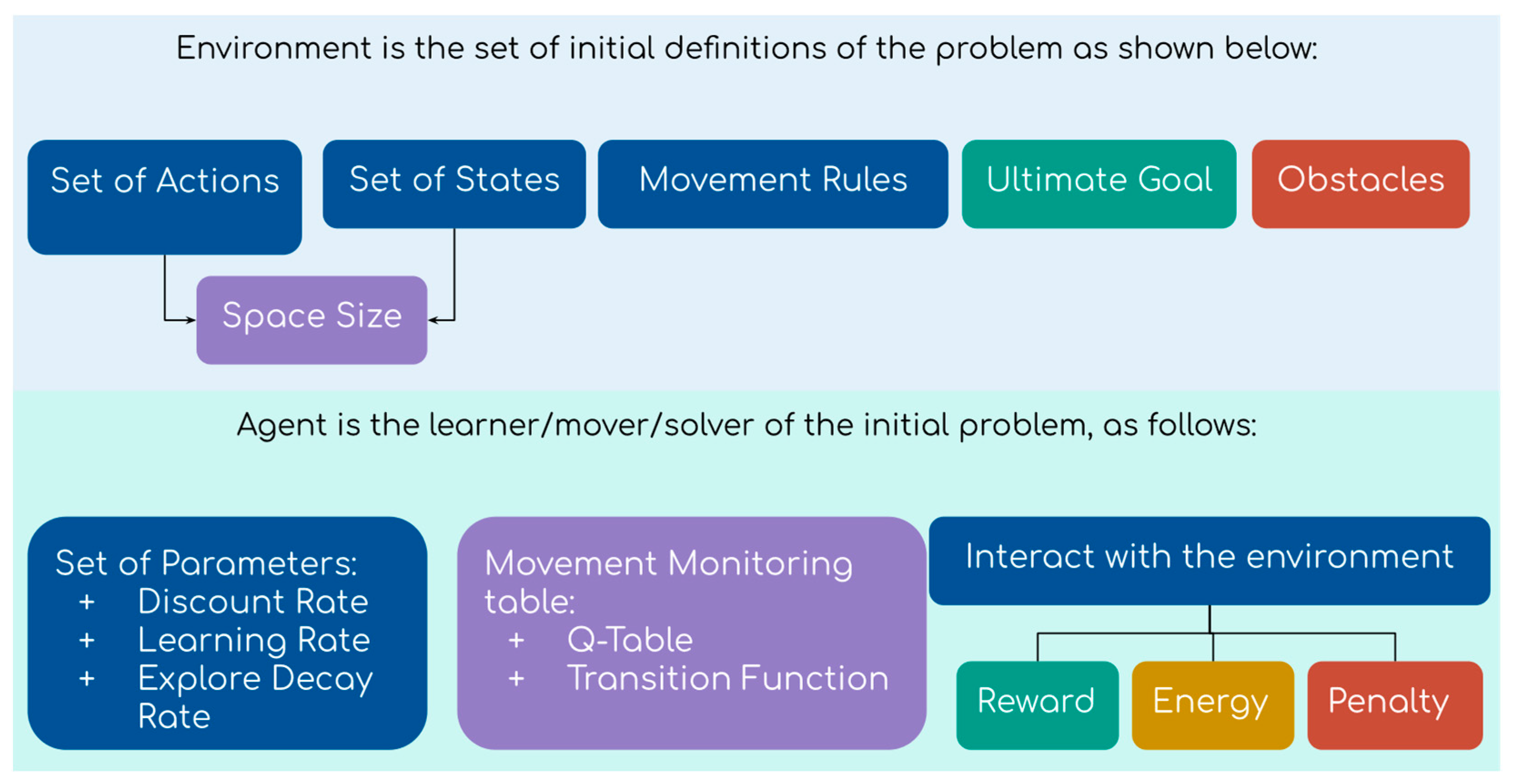
Figure 4. Each of the deep Q-networks in this article contains two hidden layers. The first hidden layer consists of ten neurons and the second hidden layer consists of nine neurons. The structure of the deep Q-networks is obtained from our preliminary testing. The goal of the Double DQN is to find the model that minimizes the error, measured in terms of mean squared error. For the Double DQN, the environment is defined as all data points in the training set and the state is the set of previous actual demand, seasonal index, month, year, number of days in a month, number of holidays, and demand trends of the previous three months.
A state
S of the environment at time
t is define as
, which is associated with a data point in the data set and is described in the Training Set block in
Figure 4:
: Actual demand in month
: Actual demand in month
: Actual demand in month
: Actual demand
: Seasonal index at month
The set of actions A in each state contains choosing one of the three forecasting models. This set of actions is the same in every state in the environment.
After the selection, the agent takes one step forward to the next state, i.e., next month. When starting at a specific month, the agent has to follow the time direction; moving backward is not allowed.
By estimating a reasonable Q-value for each prediction method in different states using the online Q-network (Q), the agent aims to maximize its total reward. Specifically, the online Q-network (Q) is updated at every step and used to select the best forecasting model each month by comparing its Q-value. The target Q-network updates weight and bias from the online Q-network (Q) every pre-specified update target period. The update period is obtained by observing results from empirical experience. This process is illustrated in
Figure 4, where the Q-network updates the weights and bias from the experience replay, then the target Q-network is periodically updated by the Q-network, while in the experience replay, the target Q-network is used to calculate the Q-value of the next state. The experience replay will be explained in the following paragraphs. The Q-value of the agent at the state
taking action
is iteratively updated by the formula from the Bellman equation [
37]:
The reward function takes the navigation role in the agent’s learning path. Using a proper reward strategy reduces the probability of falling into a local optimum solution and quickens the convergence speed. In forecasting problems, it is common to give rewards based on prediction errors such as square error or absolute error. However, in the model selection problem, a reward function needs to consider all the predicted values of the three models. At a certain month, one forecasting model might substantially outperform others. The agent should receive more rewards in those critical selections. In this paper, the reward function based on the performance difference of the selected forecast values is presented as follows.
From Equation (11), choosing the best prediction value from Model 3 results in a positive reward of . On the other hand, choosing the worst prediction value from Model 1, the agent obtains the negative reward of .
The experience replay is an important technique in the Double DQN. The functional purpose of this technique is to break the correlation of sequential data and ensure the sample is independent and identically distributed. In the experience replay, the agent’s experiences are saved as tuples and appended in the replay memory. Each tuple
includes the environment state
t, action taken at state
t, reward from state-action pair
t, and the environment of the next state.
The experience replay also helps to justify the estimation of future value using the predicted values from the target Q-network, which prevents the agent from optimistic overestimation. It is required that the agent passes through at least a number of data points equal to a batch size to initialize the experience replay.
In this study, a stopping condition was added once the agent was eligible for the experience replay to reduce the training time. The prediction error from agent actions in each step is stored for accumulated MSE calculation. A threshold was set as the maximum MSE that can be accepted for this study. If the accumulated MSE is greater than the threshold, the results from the current online Q-network are used to compute the mean squared error for the whole training set to compare with the threshold again.
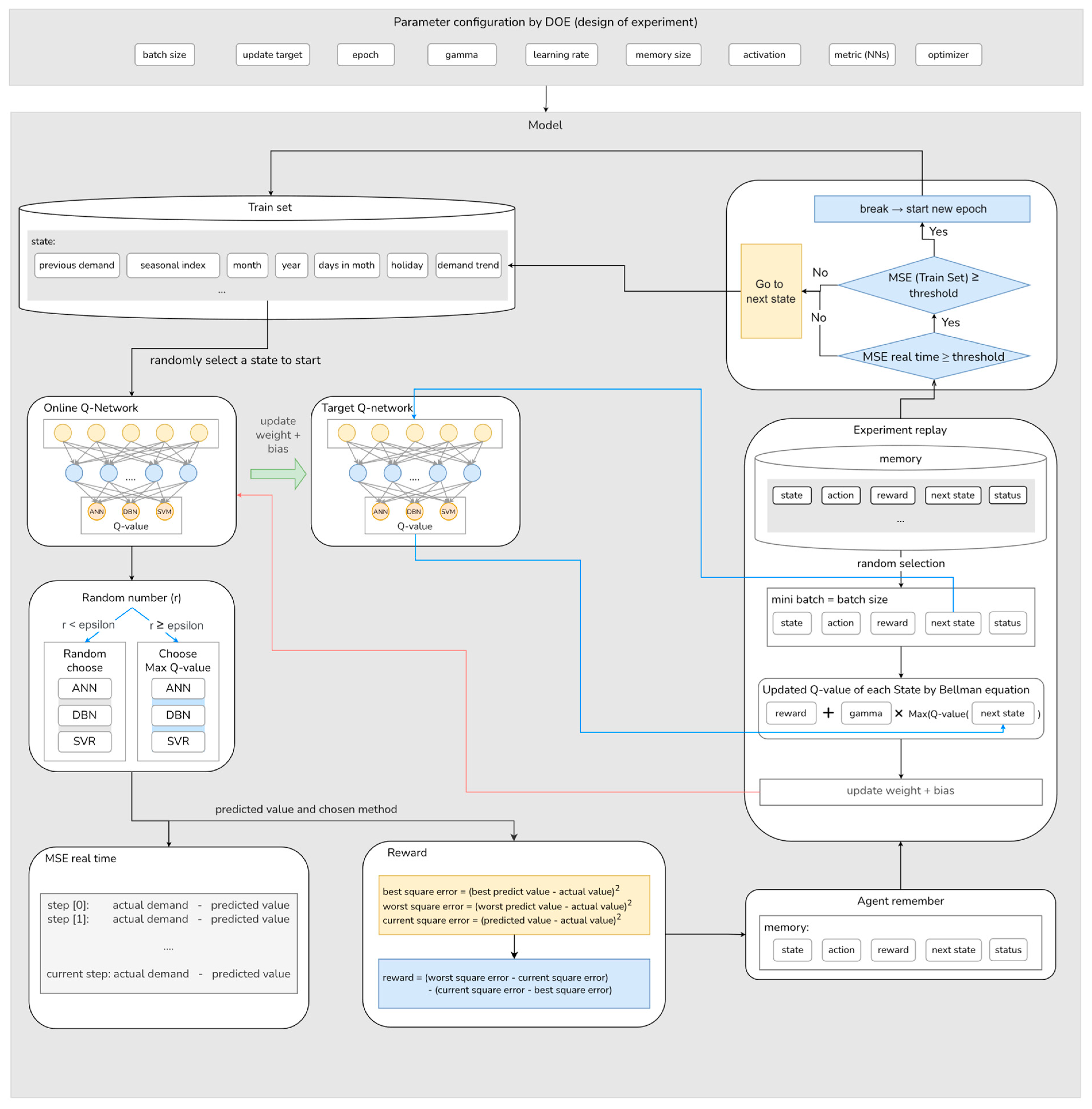
The diagram in
Figure 4 illustrates the training process of the Double DQN, which involves tuning ten hyperparameters of reinforcement learning using the fractional factorial design technique. The training set consists of states, each of which contains various features, such as previous actual demand, seasonal index, month, year, number of days in a month, number of holidays, and demand trends of the previous three periods. To initiate training, the agent randomly selects a state and proceeds without the ability to go back to the previous period. At the beginning of the training process, when the exploration rate (epsilon) is high, the agent explores different forecasting models by randomly selecting from a pool of three machine learning models. As the agent gains experience and knowledge, a lower epsilon value promotes exploitation, focusing on actions that have yielded higher long-term rewards. The agent is more likely to choose the forecasting method with the maximum Q-value.
After taking an action, the real-time MSE between the predicted and actual values is calculated and stored. The reward for the chosen action is determined by comparing the squared error of the selected method with the most accurate and least accurate methods among the three forecasting models. The state, the chosen forecasting method, the reward, and the next state are recorded in a tuple () and stored in the agent’s memory for experiment replay. The capacity of the agent’s memory is a hyperparameter, called “Memory size,” which is also tuned using the fractional factorial design technique.
During the training process, the agent randomly samples a mini-batch, equal to the batch size, from its memory. For each experience in the mini-batch, the Q-value is updated using the Bellman equation, and the weights and biases of the Q-network are updated accordingly. The Q-value of the next state is calculated using the target Q-network (a separate duplicate of the online Q-network), which is periodically updated based on the tuned “Update target” hyperparameter.
After the experiment replay process, both the real-time MSE and the MSE of the entire training set are compared to a threshold, which represents the specified maximum acceptable MSE. The MSE of the entire training set is calculated by using the current online Q-network to select forecasting models and compute the MSE. If both MSE values exceed the threshold, the agent proceeds to the next step in the training set. Otherwise, the agent starts a new epoch using the current weights and biases of the Q-network. After the final epoch, the weights and biases of the Q-network that result in the best MSE on the entire training set are saved as the final model of the training process.
3.3. Hyperparameter Tuning of the Double DQN
Hyperparameter tuning is crucial for machine learning techniques since it can improve model performance when changing the model structure is costly and time-consuming. There are different approaches to tuning hyperparameters. One of the most preferred by researchers is called grid search, which tries all possible combinations of hyperparameters [
51]. However, this technique requires an exhaustive search operation if the number of hyperparameters is large. In this study, the fractional factorial design was used to tune a set of hyperparameters affecting the Double DQN model performance with an acceptable computational time required. The considered hyperparameters in this study include batch size, update target period, epoch, gamma, learning rate, memory size, activation function, metrics inside the neural network, and optimizer. The range of each hyperparameter of the Double DQN is shown in
Table 1.
The batch size determines the number of data points fetched from memory during the experience replay. The range value of batch size is based on a trade-off between computational time and prediction accuracy, as a large batch size has faster training time but poor generalization, and vice versa [
52]. The update target controls the relative length of the period, after which the target Q-network replicates the parameter configuration of the Q-network (Q). Memory size determines the number of tuples that can be stored in the replay memory with the rule that the newer memory replaces the oldest memory. In this study, two state-of-the-art activation functions, rectified linear unit 6 (ReLU6) and sigmoid-weighted linear units (dSiLU), are compared [
53,
54]. For optimizers, rectified Adam and stochastic gradient descent (SGD) were potential candidates. Rectified Adam inherits Adam’s performance speed while improving the robustness of the training phase, whereas SGD has the advantage in prediction quality, particularly the test set accuracy [
55]. The metric (NNs) indicates the measurement of the accuracy of the neural network’s internal estimation, which does not refer to the prediction error between predicted and actual demand.
Using the fractional factorial design, a total of
runs with some center runs are generated, where
represent the number of hyperparameters as presented in
Table 1 and
indicates the fraction of the full factorial. After the Double DQN model is trained with the generated hyperparameter settings according to the fractional factorial, a statistical analysis was carried out to identify the sets of hyperparameters that yield the best MSE. Based on the obtained set of hyperparameters, the Double DQN model is re-run five times for confirmation purposes. The final Double DQN model is selected based on the best performance in the test set.


