Semantic-Aware Path Planning with Hexagonal Grids and Vehicle Dynamic Constraints

Abstract

The article presents a navigation system that utilizes a semantic map created on a hexagonal grid. The system plans the path by incorporating semantic and metric information while considering the vehicle’s dynamic constraints. The article concludes by discussing a low-level control algorithm used in the system. This solution’s advantages include using a semantic map on a hexagonal grid, which enables more efficient and accurate navigation. Creating a map of allowable speeds based on the semantic map provides an additional layer of information that can help optimize the vehicle’s trajectory. Incorporating both semantic and metric information in the path-planning process leads to a more precise and tailored navigation solution that accounts for the vehicle’s capabilities and the environment it is operating in. Finally, the low-level control algorithm ensures that the vehicle follows the planned trajectory while considering real-time sensor data and other factors affecting its movement. Through this article, we aim to provide insights into the cutting-edge advancements in path planning techniques and shed light on the potential of combining hexagonal grids, vehicle dynamics constraints, and semantic awareness. These innovations have the potential to revolutionize autonomous navigation systems, enabling vehicles to navigate complex environments with greater efficiency, safety, and adaptability.

1. Introduction

In recent decades, the market for autonomous unmanned ground vehicles (UGV) has grown in many countries. However, we believe that the off-road environment is the most challenging aspect of autonomous UGV navigation. In the real world, autonomous navigation becomes significantly more complex with uneven terrain, lack of drawn lines, presence of other agents, and absence of structured objects. As a result, an effective autonomous system capable of controlling UGVs in unknown environments must be complex and have access to as much information as possible.

Path planning algorithms are pivotal in enabling vehicles to autonomously determine optimal paths to their destinations while considering various constraints and objectives. To address this challenge, researchers and engineers have been exploring innovative approaches to path planning, incorporating advanced techniques such as hexagonal grids and semantic awareness.

Traditional grid-based path planning algorithms have primarily relied on square grids to represent the environment. However, hexagonal grids offer several advantages over their square counterparts. Hexagons provide a more natural representation of the physical space and allow for smoother and more realistic paths. Moreover, hexagonal grids exhibit better connectivity properties and more efficient use of computational resources, making them an appealing choice for path-planning tasks.

Another crucial aspect of path planning is the incorporation of vehicle dynamic constraints. Autonomous vehicles need to adhere to the physical limitations of their motion, such as acceleration, to ensure safe and efficient navigation. Integrating these constraints into the path planning process is vital to avoid collisions, minimize energy consumption, and optimize the overall vehicle performance. In recent years, researchers have recognized the importance of semantic awareness in path planning. Semantic information about the environment can greatly influence the decision-making process of autonomous vehicles. By incorporating semantic awareness, vehicles can consider contextual information and adapt their paths accordingly, enhancing safety and efficiency.

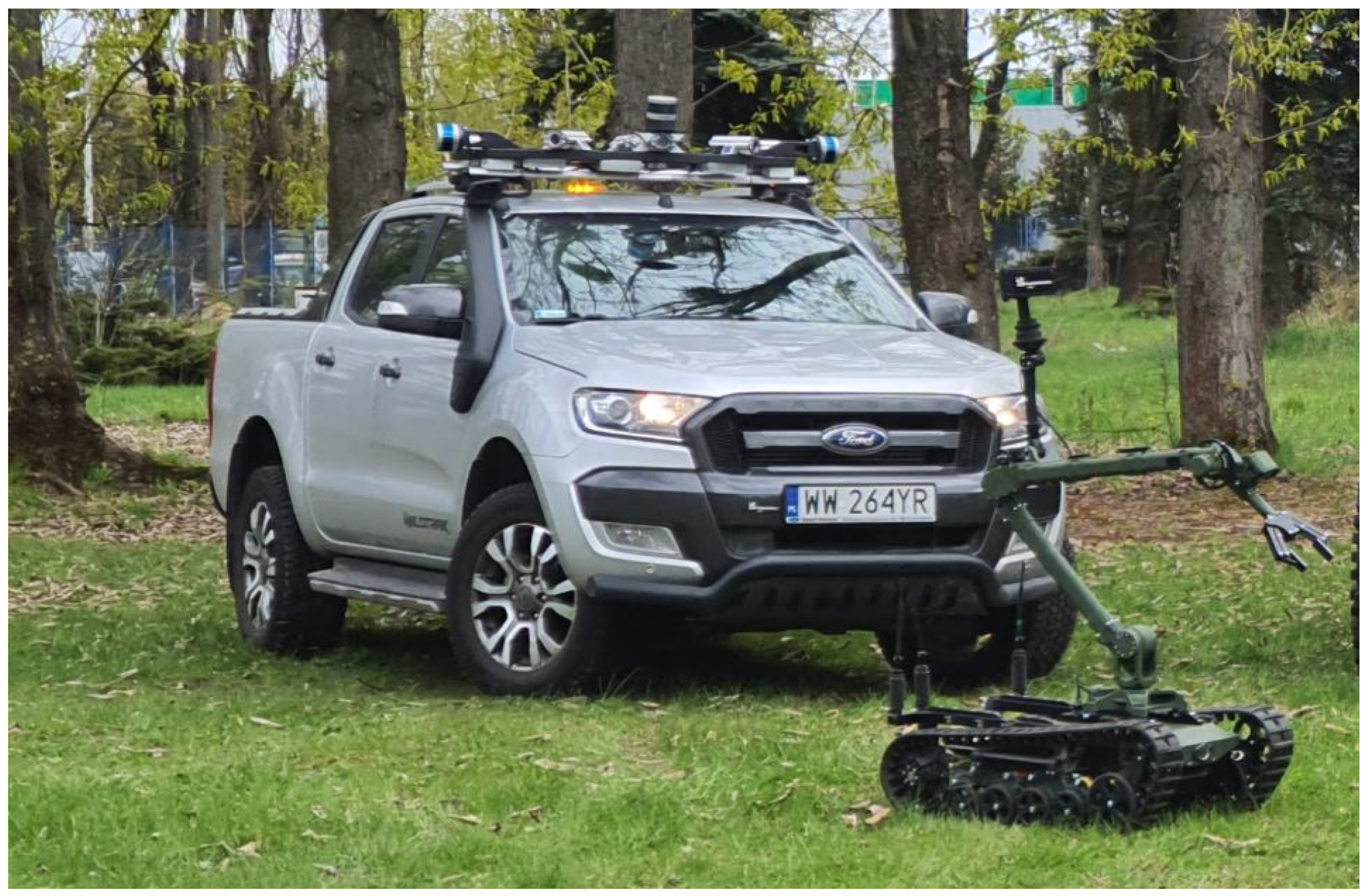
Research on this type of autonomous system at the Łukasiewicz Research Network–Industrial Research Institute for Automation and Measurements PIAP has been conducted since the launch of the project in 2018, called ATENA. For now, the project DEZROB—the comprehensive tool for disinfection of rooms and pedestrian routes built on a UGV, which contains an autonomy module—is continuing the research on the traversability estimation and autonomous path planning for the Łukasiewicz–PIAP UGVs. In the DEZROB project, we need to expand the Łukasiewicz–PIAP ATENA autonomous system by adding to the path planning algorithm, the ability to plan the clear path for the mid-size UGV–Łukasiewicz–PIAP PATROL; both platforms are shown in Figure 1. In the DEZROB project, we built a new autonomy controller and used new sensors. However, we use the same algorithm developed in the ATENA project. The algorithm is still in the development phase, and the goal is to implement the autonomous functions in the specified Łukasiewicz–PIAP UGVs. The complete DEZROB system will have a particular disinfection function that allows autonomous disinfection in the rooms and halls. This article focuses on the autonomous navigation of the Łukasiewicz–PIAP UGV implemented on DEZROB and ATENA systems. The main differences between those systems are the scale of the autonomous controller. In the DEZROB project, we use the autonomy controller based on the SoM, which is more energy efficient than the autonomy controller used in the ATENA system based on the standard computer components built in the high-strength case. The main difference besides the dimensions and weight between ATENA and DEZROB is the holonomic base of the DEZROB and the usage scenario. DEZROB will work in the indoor environment, but as a small UGV with an autonomy controller, it is convenient to conduct research for this article with autonomous path planning in the outdoor environment.

The ATENA system and sensors were described in [1]. In the DEZROB system, the sensors are slightly different. The ATENA was originally designed to work with large UGVs such as autonomous cars and 3.5 ton Łukasiewicz–PIAP HUNTER UGV. The differences in size and type of UGV can be clearly seen in Figure 1. Because of its size, the ATENA system uses multiple LiDARs and cameras. The Łukasiewicz–PIAP Patrol used in the DEZROB project, shown in Figure 2, is equipped in 360 deg. LiDAR Ouster OS-1 (64 layers), 120 deg solid-state LiDAR LSLIDAR CH128 (128 layers), the 3d cam ZED3D 2i, and for outdoor path planning with environmental material recognition, it can be equipped with a hyperspectral camera Cubert Q285.

To unify the autonomous system for Łukasiewicz–PIAP UGVs, we implemented parameter models of our UGVs in the system. We assumed that the autonomous algorithm would be the same, but the input data for the traversability estimation will be specified for each UGV model.

Besides these model parameters, adding the dynamics calculation to optimize path planning is required because of different weight and dynamic characteristics, which can occur on different types of Łukasiewicz–PIAP UGVs and even of various versions of the same UGV. For instance, the DEZROB version of the Łukasiewicz–PIAP PATROL is equipped with a manipulator with nozzles and a tank with pumps for the disinfection liquid, which significantly extends the mass of the UGV with a full tank.

Traversability estimation in autonomous UGV is one of the critical abilities in a wide range of unmanned missions. The UGV, planned for use in military scenarios as a logistical, surveillance, or combat vehicle, must have an autonomous onboard algorithm to handle real-time path planning in rough terrain. The ability of the algorithm to predict mobility increases the survivability of the UGV on the mission. If UGV becomes immobilized, the mission will be jeopardized or even failed. In Łukasiewicz–PIAP, we are developing the UGVs for special forces, including military use. Because of that, our future autonomous algorithm implemented in our products must be robust and work predictably for the mission planner. Our motivation is to develop autonomous systems fully operating in off-road terrains.

Across the projects ATENA and DEZROB, we want to develop a universal autonomous algorithm designed to work with various Łukasiewicz–PIAP UGVs in challenging terrain, considering the terrain conditions and abilities of the UGV to traverse the terrain. In [2], we developed the hexagonal grid map that speeds up and improves local path planning. In [1], we prove that we developed an effective classification method of the materials in the environment based on the hyperspectral camera. We described the path planning with the map of the environment with a cost function—the value of the grid depends on the type of ground detected. Now, we are describing a path planning method with these methods and extend with the vehicle dynamic constraints. Using dynamics, the extension improves our autonomous algorithm by reducing the risk of being stuck in the terrain. Additionally, it allows us to use it in a broad class of the UGVs (grouped by mass: Łukasiewicz–PIAP Patrol with DEZROB accessories, 100 kg; Łukasiewicz–PIAP IBIS, 300 kg; Łukasiewicz–PIAP ATENA, 2200 kg; Łukasiewicz–PIAP HUNTER, 3500 kg. The mass of UGVs is an approximation; specific mass depends on accessories and payload). We standardize the control algorithms of our UGV system. The development of dynamic-based path planning, described in this article, is a step further in making it happen in the autonomous operation of our UGVs.

This paper is organized as follows: following the introduction is the section discussing related work. In Section 3, the mapping method is described. Section 4 presents the velocity constraints used in path planning. Section 5 describes the path planning process with speed constraints using our mapping method. We briefly explain the low-level control that calculates the path the UGV will follow. Section 6 presents our experimental results. The article concludes with a summary and bibliography.

2. Related Work

The work aims to develop an algorithm for the navigation of a mobile robot that creates a terrain map with information on the ground material and plans a path considering the ground structure and the robot’s dynamics.

2.1. On Navigation of Robots

In the navigation of mobile robots, it is necessary to have a model of the environment, be able to observe the actions taking place in the environment, know the robot’s location in the environment, and plan the path while performing actions. Such an approach could be called a classic model. It is based on metric or topological maps, which only store information on whether a map cell is free or not (in 2D or 3D space) or whether a graph node is passable. Additionally, the robot is imagined as a material point without dynamic and kinematic constraints. The map can be given in its entirety or created on an ongoing basis. Dynamic obstacles may also appear on a known map (the environment changes dynamically). The certainty of information about the environment can also be considered by using the probability of certain events, e.g., the degree of certainty that a given map cell is occupied, the uncertainty of the robot’s position in space, etc. A general overview of mobile robot control and navigation can be found in [3]. More on metric and topological maps can be found in [4].

However, this is a very general system that does not consider many variables, such as differences in ground passability, slope, the feasibility of turns, width of passages, ground adhesion, achievable speeds, and accelerations of the robot.

2.2. Path Planning in Unknown Environment

The problem of route planning with incomplete knowledge of the environment, simultaneous map creation and localization (SLAM), completeness, and optimality of the planned path are well described in the literature for the classical model. For route planning in a dynamic environment using genetic algorithms, see [5]. The combination of genetic algorithms and Q-learning is described in [6]. Another example of using Q-learning for a dynamic environment is in [7,8]. The use of the particle swarm optimization algorithm is described in [9]. Implementing the A* algorithm in three-dimensional space (for a flying craft) is described in [10]. An example of using the ant colony algorithm is in [11]. Route planning in rough, challenging terrain using deep reinforcement learning was demonstrated by Shirel and Degani in [12]. The same method is used in [13]. The vision-based path planning system for uneven terrain for the lunar rover is described in [14].

2.3. Semantic Maps

Semantic map navigation is an approach for dealing with gathering, processing, and using information about the environment. The semantic map contains information about the nature of the environment, e.g., type of ground, suitability for passing, etc. [15,16]. Such information can be used in path planning to impose, for example, an additional cost for driving over uneven terrain. This allows us to search for a path that is optimal not only in terms of length or time but also in the vehicle’s dynamic capabilities. The process of building a semantic map using artificial labels on objects is shown in [17].

Among the many methods of obtaining data on the environment in order to build a map, there are rangefinders, LiDAR laser scanners, or those based on cameras with stereo vision [18].

Those that are useful for building a semantic map (i.e., they carry information about not only geometry) are, for example, RGB cameras, where objects can be classified using, for instance, artificial intelligence methods, YOLO, and ResNet [19]. Building a map with LiDAR is conducted by projecting a point cloud onto a surface, as shown by [20,21].

2.4. Hexagonal Grids

The use of square cells in grid-based representation has some drawbacks. The distance between the center of a cell and the center of a diagonally adjacent cell is greater than the distance between the center of a cell and those it shares an edge with. Additionally, neighboring cells may not always share edges, as diagonal cells only touch at a single point. Representing curved shapes accurately on a rectangular lattice is difficult.

In biological vision systems, such as the human retina, photoreceptors are arranged in a hexagonal lattice. Hexagonal grids have several advantages over square grids, as shown in studies [22]. Firstly, the distance between a cell and its immediate neighbors is the same in all six primary directions. This results in more accurate representations of curved structures compared to rectangular pixels. Secondly, a smaller number of hexagonal pixels are required to represent the same area on the map, which can reduce computation time and require storage space. Moreover, studies [23,24] have demonstrated that hexagonal sampling leads to a more minor quantization error for a given resolution capability of the sensors.

Research [25] has shown that hexagonal grid map representation is superior to quadrangular grid map representation for cooperative robot exploration. However, this research did not consider the problem of collision-free path planning in a real environment. The use of hexagonal grids is also described in our paper [2].

2.5. Dynamic Constraints

In order to implement navigation algorithms on a mobile robot, the robot’s dynamic and kinematic constraints must be considered. These limitations may be external or internal. External is ground adhesion, friction, road width, curve radii, slope, and unevenness. The internal ones are the ability to achieve a given speed and acceleration, the robot’s maneuverability, and suspension [26]. The topic of dynamic limits in mobile robotics and taking this into account has been of interest to researchers for a long time [27].

There are many papers, including recent ones, which analyze, for example, the dynamics of the power source in order to better manage energy under changing load conditions [28], but these works do not take into account the environment model in a strict way, as our work does. At this point, it is also worth mentioning research in which attempts are made to implement control systems for autonomous vehicles based on predictive controllers [29]. In this work, the proposed system provides a more balanced load for the separate drives of the vehicle, regardless of the path taken by the robot. Although the work is verified with a simulation in Matlab, it is an example of a different approach than ours. Savings in the vehicle’s operation are sought through the method of control and not by recognizing and modeling the environment.

Route planning in a static environment with dynamic obstacles for a robot with a simple kinematics model is described in [30]. The authors also present the trajectory generation algorithm using the robot kinematics model. A similar example is in [31]. Numerous papers describe kinematic and dynamic constraints for lunar rovers, e.g., [32].

Much has been said about robot kinematics in [33]. Rosman et al. propose an algorithm optimizing the trajectory of a car-like robot.

2.6. Traversabilty Estimation

In complex and challenging environments, dividing the terrain simply into free and occupied cells is often impossible. However, it is necessary to determine the degree of traversability depending on the nature of the ground [34]. The map that describes the surface of the mobile robot can be defined as 2.5D. An example of building such a map and determining the robot’s path can be found in [35]. The article [36] describes an algorithm for navigating a robot in an uneven environment in a confined space with ramps and stairs. The authors build a 3D map of the environment with passability estimation. In the previously cited work [31], traversability is analyzed as well. Paper [37] also analyzes the traversability on a metric map created from a point cloud. Passability analysis for a mobile robot on a semantic map is also described in [1]. Methods of estimating terrain unevenness were presented by researchers in [38,39].

2.7. Semantic Maps, Path Planning, and Dynamic Constraints in One Approach

The scope of this work is a combination of all aspects mentioned above: metric and semantic maps and the constraints in the robot’s dynamics and kinematics at the route planning stage. We obtain data from a hyperspectral camera and LiDAR.

Taking the robot’s speed into account for navigation is necessary due to the limited ability of the drive system to transfer power (speed cannot change in abrupt steps) and helps to drive through, for example, sandy areas, where the required speed is usually higher to prevent the robot from getting stuck in the sand. Therefore, the cost of travel due to the length of the route may be the same for sandy and paved terrain. However, considering the driver’s ability to achieve the necessary torque to accelerate the robot, it may turn out that the sandy route is less profitable.

Among the various papers dealing with path planning on semantic maps, one can mention the route planning for an aircraft using the semantic map [40]. Scientists use optical flow to detect and classify obstacles and a modified rapidly-exploring random tree (RRT; more about it in [41]) for navigation. However, the algorithm does not consider the limitations of the drone’s dynamics. A similar solution is in [42]; the researchers use photogrammetry to build a three-dimensional map of the drone’s surroundings.

Wermelinger et al. developed a path-planning system in rough terrain for a four-legged robot. They use the kinematic constraints of a four-legged robot to estimate traversability. The map used in this work is not strictly semantic [43].

Zhao et al. proposed a route planning system based on a vision-based semantic map [44]. However, this approach is computationally expensive and challenging to use in real-time systems when adding a new class to the map is needed.

In work [1], we showed how to build a map using LiDAR and a hyperspectral camera. Data from this camera allowed for the building of a semantic map with information about the type of substrate. We used this information to determine the area’s traversability and plan the robot’s route. We used the k-nearest neighbors method to classify the ground.

Planning the movement of obstacles on a semantic map was presented by Salzmann et al. [45]. They propose an algorithm that predicts human movement in a mobile robot environment, considering the limitations of human dynamics.

None of the above works, however, consider the robot’s dynamics with a semantic map. Building such a system is a valuable approach. Semantic maps can include information about the environment at the path planning stage, so it happens before taking any action by the robot. Considering kinematic and dynamic constraints, we can generate a path for the robot, which is sure that the robot will be able to perform.

3. Mapping

Our navigation system creates a hexagonal grid-based map of the surroundings. We decided to use this kind of representation because of the following advantages:

• Hexagons tessellate the plane more efficiently than squares or triangles, meaning that they can fill the space with fewer gaps and overlaps to better approximate a curved surface.
• They have six symmetrical axes of symmetry, making them more natural for representing directional movement and capturing the orientation of biological and physical systems.
• Hexagonal grids have more neighbors per cell than square grids, which makes them better-suited systems that require more complex interactions between neighboring cells.
• The distance between any two adjacent hexagons in a hexagonal grid is the same; it is helpful in mapping and path planning (see Figure 3).
• In our paper [2], it is shown that the path planned using a hexagonal grid is shorter than using rectangular grids.

Calculating a cell’s coordinates in a square grid is a simple process. However, for hexagonal meshes, the computation is more complex. In our approach, the array set addressing method (ASA) is used [46]. This method represents the hexagonal grid as two rectangular arrays. The two arrays are distinguished using a single binary coordinate. Three coordinates uniquely represent a complete address of a cell in a hexagonal grid:

$$(a,r,c)\in \{0,1\}\times \mathbb{Z}\times \mathbb{Z}$$

(1)

where a—binary index of an array, r—row index, c—column number, $\mathbb{Z}$—positive integers.

In contrast to the classic 2.5D map in our approach, cells store a pair of values:

$$(h_{arc},labe{l}_{arc})$$

(2)

where: $h_{arc}$—represents the height of the surface; $labe{l}_{arc}$ is the semantic label describing the type of the surface. Metric and semantic information is essential in the route-planning process. The semantic information about the surface type is determined based on the hyperspectral camera.

Hyperspectral cameras capture a wide range of electromagnetic wavelengths, including those beyond the visible spectrum. This enables robots to perceive and analyze data invisible to the human eye. They can identify structural defects, anomalies, or hidden damage in objects without the need for physical contact or invasive techniques. This capability is valuable in robotic applications involving quality control. Hyperspectral imaging generates large amounts of data, as it captures detailed information across multiple spectral bands. Processing and analyzing this data in real-time require powerful onboard hardware.

Figure 4 presents the spectral response for two kinds of surfaces: asphalt and mud. The classification algorithm is described in detail in our paper [1].

The height of the surface is determined based on the indications of the laser rangefinder (LiDAR).

The point cloud can be represented as a set S.

$$S=\{x_i,y_i,z_i\}$$

(3)

where: $\{x_i,y_i,z_i\}$ are the 3D coordinates of a point.

Figure 5 presents the cloud of points obtained by the laser range finder in the outdoor environment.

The height of the surface represented by a cell is calculated based on the formula:

$$z_s=\frac{1}{n}{\Sigma }_{i=1}^n{z}_i$$

(4)

where: $z_s$—the height of the area represented by a cell in the hexagonal grid map; n—number of points assigned to the cell; $z_i$—original z coordinates for point i, which is assigned to a given cell.

Figure 6a presents the hexagonal $2.5D$ map of the environment. Figure 6b shows an enlarged portion of the area marked by a black rectangle.

The type of map described is universal and can be used by robots of any type. In contrast to classic solutions, we do not create a traversability map. Vehicle dynamics constraints (e.g., the required limiting surface angle) are considered at the path planning stage. With this approach, a map created by one type of vehicle can be used by another.

4. Region with Velocity Constraints

During navigation in outdoor surroundings, we can observe areas with velocity constrains. For example, driving at high speed on ice or mud can cause the vehicle to slip and cause an accident. The robot must slow down before entering the area with a low permissible velocity. The value of velocity stored in the cell depends on the type of terrain segment it corresponds to.

In many algorithms, the travel time affects the form of the path, but the limitations of the robot’s acceleration are considered at the low-level stage. The dynamic window approach is an example of such a method [47]. The dynamic window represents the range of allowable velocities the robot can achieve within a short interval. It is determined by the robot’s current state and limitations of acceleration. For example, the situation in which a robot switches from an asphalt road to a muddy road at high speed is very dangerous. The robot should initiate the braking process earlier. Such behavior has been taken into account in our method. We want to consider speed limits already at the path planning stage.

Figure 3a presents part of the environment. Gray cells present the area covered with concrete; black is the area covered with mud. Figure 7b presents the corresponding maximum permissible speed (80 km/h, red color; 10 km/h, blue color).

The velocity map is updated as follows:

• For each cell of the map, the corresponding value of the velocity is obtained (v);
• The neighboring cells $\left\{c_i\right\}$ are analyzed; if $v_i-v_j>a$, then $v_i=v_j+a$, where a is the maximum acceptable difference between velocities;
• The process is continued until stability, i.e., the cells will not change their values.

5. Path Planning

Considering terrain accessibility analysis when planning a route can optimize the route in terms of UGV travel cost. In our approach, we can plan a route using environmental material data, which enables us to consider the friction coefficient in the calculations. This approach makes practical route planning in hilly terrain possible, where the UGV must navigate inclines and declines. We can assume a driving scenario where the UGV encounters a rise. If the rise is covered with asphalt, the incline is achievable, but if the same rise is covered with mud, the incline may be impossible due to a low friction coefficient that prevents the incline from being passed. Many parameters that affect the UGV’s ability to pass the route must be considered. In practice, such a vehicle is limited by its maximum speed and maximum incline angle determined by the vehicle’s construction and power. Therefore, the algorithm calculating the cost of traveling on such a route should at least consider the parameters indicated in the

Table 1. Table with description of parameters that can be considered for traversability estimation for the UGV.

Parameter	Description
The angle of attack	Maximum angle at which the vehicle can climb an incline
The angle of descent	The maximum angle from which the vehicle can descend
Maximum speed	The maximum speed of the vehicle (possibly max V at a specified incline angle)
Maximum incline slope	The maximum height difference between the entry and exit points of a climb
Maximum descent slope	The maximum height difference between the entry and exit points of a descent

.

It is possible to use the above parameters to add a value depending on the vehicle’s dynamics to the travel cost function.

It is worth mentioning that in the case of different materials that make up the terrain, the coefficient of friction may not apply to the terrain’s surface. In the case of a damp terrain covered with grass, it is possible to cut the outer layer of the surface during wheel or track slippage, revealing mud, which will be the friction coefficient that should be considered during analysis. In the current version of the system, this phenomenon has been omitted. Further work on the algorithm that predicts the appropriate surface friction coefficient using data on the moisture level and composition of the ground (using the information on the susceptibility of the ground to deformation) is required.

In the described example of climbing up a hill by Łukasiewicz–PIAP UGVs equipped with the hyperspectral camera, the forces acting on the UGV have been marked in Figure 8.

The simplified dynamic equation for the robot moving uphill is given as follows:

$$F=m·a+m·g·sin\alpha -f_f$$

(5)

where:

• F    is force acting on the robot;
• m   is mass of the robot;
• a     is acceleration of the robot;
• g     is acceleration due to gravity;
• $\alpha$    is angle of the hill;
• $f_f$   is the force acting on the robot due to the type of ground, type of robot wheels, and vehicle’s mass.

The required power of the vehicle is given as follows:

$$P=F·v$$

(6)

where:

• v—the velocity of the vehicle;
• P—the power of the vehicle.

In typical algorithms, the $f_f$ parameter is not considered, and the decision of whether the terrain is traversable is made based on the slope angle. This approach is not sufficient. Equations (5) and (6) show that whether a given terrain is passable depends not only on the slope of the elevation but also on the type of surface, the type of wheels, and the engine power. In our approach, each map grid contains two values: the terrain height and the semantic label. Whether or not an area is passable is determined by both parameters together. Additionally, the type of vehicle is taken into account. The area covered with tall grass is passable, and the gentle slope covered with mud may be impassable. The terrain type also determines the maximum permissible speed, which should be considered in path planning.

This article proposes the use of the diffusion method for path planning. It generates paths faster than the RRT algorithm and allows for the easy incorporation of costs driving over different surfaces.

Based on a hexagonal grid-based map, the cost map is created. The map represents possible robot positions (states), with the robot position ($c_R$) and the goal position ($c_G$) being the two types of states distinguished. In contrast to classical path planning systems, this approach does not simply divide cells into two categories (robot accessible, occupied). Instead, an additional parameter e (cost of travel between map cells) is introduced.

$$e_{aij}^{akl}=f(h_{aij},h_{akl},s_{aij},s_{akl})$$

(7)

where:

• $aij$,$akl$—index of neighboring cells;
• $h_{aij}$—the height of the area corresponding to cell $aij$;
• $s_{aij}$—the semantic label.

The value $e_{aij}^{akl}$ depends on the slope between cells $ij$ and $kl$ and the types of cells. In our approach, the rule-based system assigns the value $e_{aij}^{akl}$.

The diffusion map is initialized by assigning an enormous value $v_G$ to the goal position cell and 0.0 to all other cells.

The value ($v_{aij}$) is calculated for each cell according to the formula:

$$v_{aij}=max(v_{aij},ma{x}_{ckl\in N^{aij}}(v_{kl}-e_{aij}^{akl}-ve{l}_{akl})$$

(8)

$ve{l}_{akl}$ is the cost of driving over cell $akl$.

This process is repeated until stability is achieved.

The resulting list of cells is then used to generate a path from the robot position to the goal position. The first cell is the robot position, and subsequent cells are chosen based on their proximity to the last cell and their maximum value of $v_{akl}$. The path generation process continues until the cell with the highest v is reached.

By introducing the parameter e, it is possible to consider vehicle dynamics already at the planning stage, and it is possible to plan the optimum speed on the individual road sections.

The Łukasiewicz–PIAP autonomy module must optimize the calculated path by the method described above (the global path) to be realized by the Łukasiewicz–PIAP UGVs. This optimization is critical to ensure the UGVs can safely and efficiently navigate their environment. The global path is the input for calculating the UGV’s trajectory in real time. The trajectory is calculated using the Łukasiewicz–PIAP autonomy module, which modifies the global path based on the size and off-road capabilities of the UGV. The low-level controller based on geometric parameters also calculates the trajectory traversable by the UGV. The trajectory is planned in a short window local map built from the environment’s point cloud. This local map provides a more detailed representation of the UGV’s surroundings, allowing for more accurate trajectory planning. The Łukasiewicz–PIAP autonomy module uses simple geometric parameters, such as the maximum slope and step of the environment that the given UGV can traverse. This controller also builds the local traversability map in the short-term window. Based on this map, the local controller uses the Hybrid A* algorithm to plan the traversable trajectory that the UGV follows. After calculating the local short-term path plan, the Łukasiewicz–PIAP autonomy module sends the steering signal to the low-level controller of the Łukasiewicz PIAP UGV. This allows the UGV to adjust its course to stay on the planned trajectory. The low-level controller works on LiDAR, odometry, and IMU sensor data. Odometry sensors provide information about the UGV’s movement, such as speed and direction, while IMU sensors measure the UGV’s orientation and angular velocity. LiDAR sensors ensure the point clouds for the traversability estimation map. This data ensures that the UGV remains on its planned trajectory, even in challenging environments.

6. Experimental Results

The experiments have been performed for vehicles: Łukasiewicz–PIAP ATENA and Łukasiewicz–PIAP PATROL.

Table 2. The specs of the Łukasiewicz–PIAP UGV used in the article.

UGV	Łukasiewicz–PIAP ATENA	Łukasiewicz–PIAP PATROL (DEZROB Version)
Ground clearance	200 mm	100 mm
Weight	2200 kg	100 kg
Turning circle	holonomic 12.7 m	non-holonomic 980 mm
Length	5389 mm	980 mm
Width	1850 mm	570 mm
Height	2015 mm	125 mm
Tire size	265/60 R18	-
Tracks	-	width 100 mm
Vmax	30 km/h	8 km/h
Approach angle	29${}^{\circ }$	38${}^{\circ }$
Departure angle	21${}^{\circ }$	38${}^{\circ }$
Max step obstacle	200 mm	250 mm

presents the parameters of the robots.

Vehicles possess diverse, dynamic constraints that necessitate distinct traversable paths to optimize their performance. Figure 9 presents the result of the experiments. Figure 9a presents the path planned for the Łukasiewicz–PIAP PATROL, and Figure 9b shows the path planned for the Łukasiewicz–PIAP ATENA.

By using semantic metric information and considering vehicle constraints, routes planned in the same environment are different for different vehicles.

Using the hyperspectral camera’s environmental material recognition in real time is limited to running in daylight. Because of the sunlight, the hyperspectral camera is inoperative at night in our system.

In practice, the system with methods from [1,2] and this article covers a wide range of situations that UGV could be challenging in the offroad terrain. The autonomous algorithm can behave like a human-operated vehicle, even when using the saved maps of the environment with the saved material’s traversability costs. The UGV using this algorithm stays on the road or flat terrain and reduces the velocity related to the terrain conditions.

7. Conclusions

The article discusses the use of hexagonal grids in navigation systems that consider vehicle dynamic constraints during route planning. Hexagonal grids provide various advantages compared to traditional grids, such as superior navigable area coverage and enhanced pathfinding abilities. They facilitate rapid obstacle detection around the robot or target and enable the inclusion of path properties, such as obstacle distance or terrain type. Moreover, hexagonal grids offer a greater number of adjacent cells than square grids, with six instead of four. Additionally, by incorporating vehicle dynamic constraints, the system can generate more efficient routes tailored to the vehicle’s specific capabilities, such as its maximum acceleration and braking capabilities. This method expands the navigation of the UGV in off-road, rough terrain. The planned path is a preliminary fit for the UGV’s off-road ability. This positively influences the ability of the mission completion by the UGV and limits situations when the low-level controller can not plan a traversable path. Considering vehicle dynamics during path planning offers numerous benefits, including improved efficiency, enhanced safety, optimal performance, realistic arrival time estimation, and adaptability to vehicle characteristics. A semantic-hexagonal map enables robots to navigate more precisely and effectively in complex environments. The introduction of semantic information enables effective route planning. Solving tasks related to action planning in the future is also possible.

Processing data from a hyperspectral camera is a time-consuming task due to the large amount of information captured across multiple spectral bands. In the future, we are going to implement dimensionality reduction algorithms and parallel processing techniques. Using graphics processing units (GPUs) can significantly speed up the data processing. This reduction in processing time will enable real-time applications of hyperspectral imaging, opening up new possibilities in various industries.

Despite the higher initial cost, the utilization of hyperspectral cameras in mobile robotics proves to be cost effective. Their enhanced perception capabilities, increased efficiency, early detection abilities, long-term investment value, and competitive advantage contribute to the overall cost savings and business benefits, making them a worthwhile investment in the mobile robotics domain. The field of hyperspectral imaging is advancing rapidly and it is expected that the cost of hyperspectral cameras will decrease over time.