Abstract
The active distribution network has been fully developed because it can achieve efficient energy utilization through the effective control of distributed generation, electrical energy storage, and active loads. However, the research on the reliability of active distribution network operation still stays in the medium and long-term calculation, without considering the influence of dynamic equipment characteristics and active distribution network operation characteristics on reliability. In order to improve the comprehensiveness and calculation speed of the reliability calculation of an active distribution network, this paper proposes a fast calculation method for the reliability of the active distribution network based on dynamic equipment failure rates. Firstly, based on fuzzy-theory and data-driven methods, the cloud model and the Proportional Hazard Model are used to model the dynamic failure rates of exposed and enclosed types of equipment, respectively. This considers the impacts of the dynamic failure characteristics of the equipment on the reliability calculation and improves the comprehensiveness of the calculation. Then, the improved K-means algorithm is used to achieve a faster and more suitable scenario reduction and increase the computation rate. Finally, considering the island operation and contact line transfer under the active distribution network, simplifying the network by improving the minimum path method, the reliability calculation method of the active distribution network combining source–load uncertainty, switch fault information, and load transfer probability is further proposed. The cases show that the dynamic fault rate model is closer to an engineering reality and has generality. The improved K-means algorithm is faster and more accurate than the traditional algorithm. The final proposed fast reliability calculation method reduces the time by 72.76 times compared to the traditional method. It fully reflects the operational characteristics of the active distribution network and provides a reference for the optimal dispatch of the active distribution network.
1. Introduction
With the rapid development of energy technology, the deep integration of information communication, and the energy industry, the active distribution network has emerged as the times require. Through intelligent measurement, information communication, and automatic control technology, the active management and control of Distributed Generation (DG), Electrical Energy Storage (ESS) and active load can be realized. Coordinated control makes intentional islanding and fault self-healing a common method to improve the continuous power supply of the distribution network and achieve efficient energy utilization [1].
In Texas, USA, in 2021, a major outage was generated due to the freezing of natural gas wellheads and ice blockages of gas transmission pipelines during cold weather and dispatching agencies did not have enough adjustable resources to maintain the balance of supply and demand. In the context of low-carbon energy transition and high penetration of renewable energy, failure scenarios need to be studied, taking into account the specific geographical environment and integrating various influencing factors. It is also important to pay attention to lightning strikes and small probability events, such as heavy rain and extreme cold. Currently, most of the treatments are divided into statistical models of fully historical failure rate data and statistical models of partially historical failure rate data by using mathematical statistical modeling based on historical failure rate data from a mathematical perspective [2]. The former performs a direct fit analysis of historical data. In [3], extreme weather strength and vulnerability curves are fitted using the minimum variance principle. The branch failure rate model is equivalent to the line pole series model. The latter compensates for the data by processing it and considering other factors. Ref. [4] chose a multi-affiliation function to describe the influence of weather factors to correct the overhead line fault rate obtained from historical statistics, but the model suffers from the disadvantages of a crude model, a vague definition of the scope, and low accuracy. In the above literature, these models generally suffer from the problems of over-simplicity of the model itself, heavy reliance on historical fault rate data, and inadequate use of multiple sources of data in the distribution network. And the practical application suffers from the short statistical time of historical data and the small sample of available data. Nowadays, the problem of insufficient statistical data is dealt with by many scholars using fuzzy-theory methods to create fuzzy sets to simulate fault situations. Ref. [5] considers the influence of the external environment on the line fault rate and expresses the line fault probability as a random fuzzy number. In fuzzy theory, the cloud model was proposed in 1995 by Academician Li Dehua as a way to deal with the randomness and fuzziness of data by accomplishing an interconversion between qualitative and quantitative concepts [6]. And Ref. [7] has improved the model evaluation method by combining cloud theory and a fuzzy model, thus realizing that the system performance can be evaluated more accurately and objectively. However, the time-varying failure rate models that currently exist have the problem of not being able to effectively handle operational data or adequately incorporate the impact of many other unmodeled risk factors and their application in reliability calculations is one-sided.
The distribution network has a complex topology and operating environment with a wide variety of equipment, which is susceptible to internal and external factors such as the operating life of the equipment, bad weather, and artificial damage [8]. It has different degrees of impact on the economy and can even undermine social stability. The rate of equipment failure in the actual distribution system is time-varying and uncertain. If the failure rate can be calculated based on multiple sources of data such as test-life data, historical outage data, and monitoring information before the equipment causes significant harm, abnormalities can be detected in time and the system can be maintained at the best time [9], which can effectively guarantee the safety, reliability, and economy of the system. Ref. [10] investigated the effects of preventive maintenance on equipment life and failure rate. In the paper [11], the age-reduction theory can quantify the impact of maintenance on equipment reliability. These methods can be effective in refining the model and making it more relevant to engineering practice but suffer from the problem of a simple model that only considers one-sided factors.
At the same time, the introduction of information systems inevitably brings new risk factors to the distribution network. During the Christmas period of 2015, due to malicious information attacks in Ukraine, some links in the power information system failed, causing regional blackouts [12]. Therefore, it has an important theoretical significance and practical demand to consider the impacts of information failure on the physical system on the basis of traditional distribution network reliability calculations. The current distribution network reliability calculation methods are mainly divided into two categories: analytical methods and simulation methods. Based on the simulation method, Ref. [13] proposes a reliability evaluation method based on the energy storage multi-state model and evaluates the load outage situation of the island microgrid through the island consequence analysis method. However, the simulation method suffers from the randomness of the random sampling process and requires a long simulation time. Ref. [14] defines the concept of an island microgrid outage sequence through an analytical method and uses an analytical method to calculate the reliability on the basis of a multi-state model of outage sequence. The probability of a blackout sequence is estimated from the combined state of DG, load, and energy storage. But the analytical method can lead to a dramatic increase in workload and difficulty with solving when the system is large. In addition, the complementary nature of simulation and analytical methods has led many scholars to investigate the use of combined approaches to alleviate the conflict between accuracy and efficiency, including the use of variance reduction techniques, such as adaptive sampling methods, space reduction techniques, such as state space reduction, and efficient computational methods, such as intelligent learning [15]. The literature [16] proposes a method for a distribution network reliability calculation based on state space classification, performing scenario reduction, and combining machine learning with Monte Carlo methods to reduce the amount of topological analysis required by conventional reliability assessment methods. However, it lacks extensibility validation in complex networks. Therefore, it is another focus of this paper to address the problems of the existing calculation methods and to consider new reliability influences while ensuring adequate computational efficiency and computational extensibility.
In order to cope with the lack of equipment reliability modeling in active distribution network reliability calculations and the bias towards the study of medium- and long-term steady-state reliability, a fast calculation method of active distribution network reliability based on equipment dynamic failure rates is proposed to introduce the failure probability of equipment and switching control information failure into the fast calculation of the distribution network reliability and improve the accuracy and speed of active distribution network reliability calculations. The contributions of this paper are as follows:
- A dynamic failure rate model for equipment that can adapt to short-, medium- and long-term scales is proposed, which is based on data-driven and fuzzy theory combined with equipment condition assessment and improved age-of-service model to differentiate the failure rates of environmentally exposed equipment and environmentally closed equipment, thus improving the accuracy and credibility of reliability calculations.
- The K-means algorithm is combined with the Sparrow Search Algorithm (SSA) for the extraction of typical scenarios of source–load rate in three dimensions. The selection of the clustering center and the number of clusters are optimized compared to traditional clustering methods and the clustering speed is improved. This reduces the amount of reliability calculation for active distribution networks and increases the reliability calculation rate.
- In the calculation of reliability indexes by the minimum path method, the equivalent average outage duration in the downstream area of the fault is modified by considering the failure of switch information. Considering the probability of load transfer, the analytical model for the reliability calculation for common users and transferable users is established, which improves the calculation rate and reliability of reliability calculation.
2. Time-Varying Failure Rate Model of Equipment
The calculation of equipment failure rate is influenced by a complex coupling of multi-dimensional and multi-physical domain characteristic parameters, which are characterized by randomness and still incomplete and unclear expressions of physical analytic equations. In this chapter, a dynamic failure rate model for equipment is developed based on fuzzy theory and data-driven methods according to the common lifetime distribution of equipment and multiple sources of data from the distribution network.
2.1. Theoretical Basis of Mode
2.1.1. Equipment Failure Rate Model
Different lifetime distributions are usually used for fitting analysis in reliability analysis, such as Poisson distribution, Normal distribution, Weibull distribution, etc. This paper only considers the degradation of the equipment and uses a phased dual Weibull distribution to describe the failure rate of the equipment, as follows:
where T1 is the start time of the stabilization period; and T2 is the start time of the aging period.
2.1.2. Proportional Hazard Model
The Proportional Hazard Model (PHM) is widely used in origin reliability fields [17] and has been gradually used in reliability analysis of power systems in recent years. According to the definition, the expression is as follows:
where is the benchmark failure rate function; is the covariate vector reflecting different states of different equipment; is the covariate vector parameter; and is the covariate connection function.
2.2. Exposed Equipment Failure Rate
Because of the exposure of the main functional components of exposed equipment to the outside environment, external factors are the main cause of its failure.
2.2.1. Weather Conditions
It is difficult to evaluate weather conditions, so the two-state weather model [18] or three-state weather model [19] are mainly used to study equipment failure rates. According to years of data from the power sector, the weather factors that cause environmentally exposed equipment failure are generally risk factors [20]. If a weather factor exceeds a threshold value to become the most dominant risk factor, the equipment failure rate model should be represented by the component susceptibility curve associated with that weather factor [21]. The deduction of points for weather conditions in different areas is shown in (3).
where is the number of failures of the j meteorological factor under the level bj; and is the total number of times the j meteorological factor has the level bj.
The final weather condition score is shown in (4).
where indicates the deduction of each factor; and is the importance of each factor.
2.2.2. External Force Damage
According to [22] and the relevant power supply reliability evaluation regulations, external force damage is divided into seven categories. S2 is introduced to evaluate the impact of each factor on the external damage health degree. A higher score indicates a lower likelihood of external damage.
where is the score of the j factor; and is the important degree of the j factor.
and are based on the discriminant matrix of each indicator given by the expert group or decision maker and the initial weights are determined using hierarchical analysis. Then the entropy weighting method is used to correct the weight vector obtained from the previous subjective weighting. This treatment avoids human subjectivity to a certain extent.
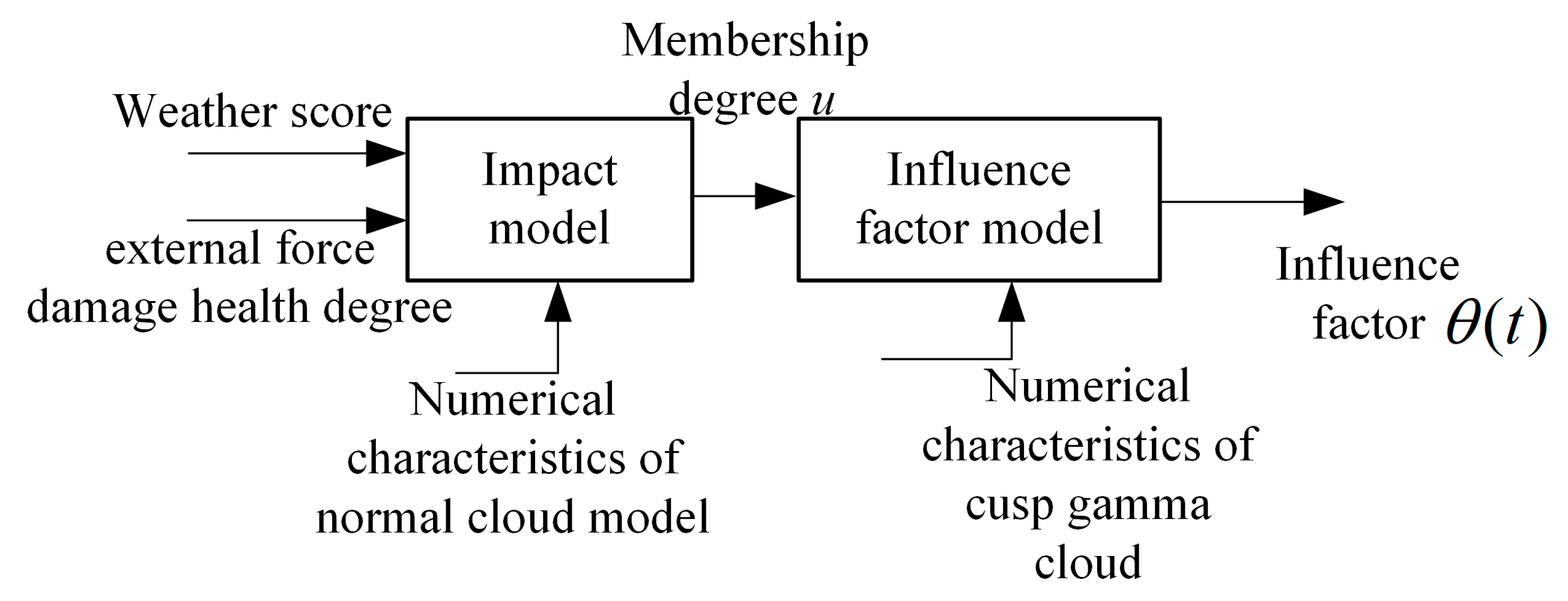
2.2.3. Two-Condition Cloud Model
Due to the random and uncertain nature of weather conditions and external force damage, the comprehensive impact factor θ is usually smaller when both weather condition score S1 and external damage health S2 are excellent. In this paper, we construct the two-condition cloud model as shown in Figure 1 to achieve the uncertainty inference prediction of the impact factors.
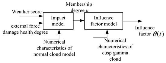
Figure 1.
The framework of two-condition cloud model.
In summary, the model of dynamic failure rate for exposed equipment is as follows:
2.3. Closed Equipment Failure Rate
Internal factors and the operating environment are the main causes of the failure of the enclosed equipment. According to the Health Index (HI) theory, which is based on the evaluation of the real-time operating status of the equipment, this paper introduces the Comprehensive Health Index (CHI) combined with PHM to jointly construct a failure rate model of closed equipment.
CHI is related to the geographical location, equipment load, equipment family, and human error, in addition to the condition of the equipment itself. The calculation formula is shown as follows:
where , , , and are the correction factors, which are taken from [23] and are shown in Table 1.

Table 1.
Reference value of correction factor.
So, the model of dynamic failure rate for closed equipment is
2.4. Correction of Failure Rate Considering Overhaul
Based on the serviceability of the equipment, it is possible to increase the availability of the equipment and improve its condition through equipment maintenance. However, equipment maintenance does not achieve a complete repair of the equipment, and as the time of use and the number of repairs increase, the equipment will suffer from maintenance fatigue.
As a result, with the appearance of maintenance fatigue, the recovery effect of the equipment after the repair is diminished and the age-reduction increment is attenuated. Assuming that has linear attenuation characteristics, and the attenuation is k, so, the age-reduction increment between two adjacent maintenances is
where .
The age-reduction amount after the i overhaul is
The equivalent age of the equipment is
So, the failure rate of the equipment after maintenance is
2.5. The Process of Failure Rate Calculation
Combined with the above theoretical basis, the solution process for the model of the dynamic failure rate of power equipment proposed in this paper is shown in Figure 2. Firstly, input the statistical data of the equipment and classify the equipment according to different equipment working conditions and operating environments. Then, calculate the current equivalent service life of the equipment by considering the influence of equipment maintenance. Finally, use the Levenberg-Marquardt method to solve the dynamic failure rate of the equipment.
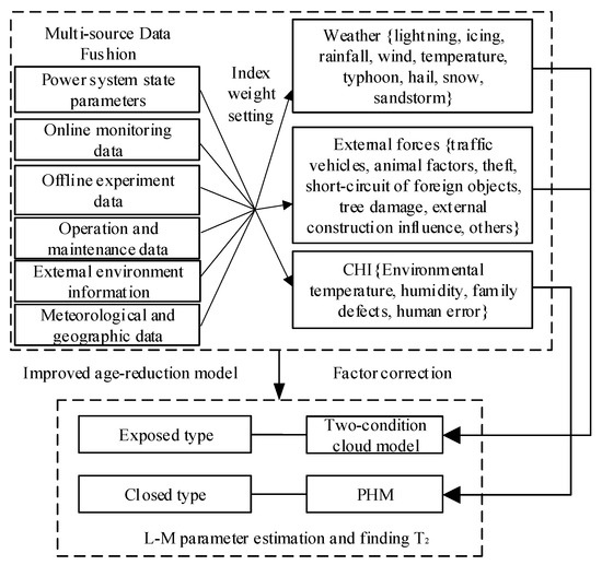
Figure 2.
The process of building a dynamic failure rate mode.
3. Fast Calculation of Distribution Network Reliability Based on Typical Scenarios
In the DG-accessed power system, wind power, and PV output are highly volatile, stochastic, and spatially and temporally correlated. Therefore, it is not reasonable to regard the relevant parameters as constants when performing reliability calculations. Accurate and effective reliability calculation methods are thus needed to show the uncertainty of DG while ensuring the efficiency of the calculation. With the application of active control strategies in the distribution network, there is a requirement to account for the rejection of control switches due to command failure when studying the impacts of switches on load points. At the same time, the minimum path method of the analytical method has a high computational efficiency, and it is easy to analyze the impact of switching states on user reliability. Therefore, this paper reduces the reliability calculation scenario and describes the uncertainty of the source–load and the dynamics of failure rate by extracting a typical source–load-rate scenario. Then, on the basis of the common reliability calculation method, the calculation process is simplified using the minimum path method combined with the network equivalence method. Finally, scenario reduction and simplification of the calculation process are combined to improve the rate of distribution network reliability calculations.
3.1. Reliability Calculation Based on Typical Scenarios
Typical scenarios include the equipment failure rate, in addition to wind power, PV, and load power. Meanwhile, DG output, load, and failure rate are all affected by environmental factors and have certain correlations and time series. In this paper, the SSA-K-means method is used to extract three-dimensional typical scenarios and effectively combine the intrinsic connection among the three.
3.1.1. SSA-K-Means Method
The K-means algorithm has the advantages of simplicity, fast convergence, scalability, and high efficiency. However, the algorithm has the disadvantages of difficulty in determining the number of clusters and inaccurate selection of the initial cluster center, which will lead to the clustering results falling into local optimality. At the same time, through comparison with other swarm intelligence algorithms, the Sparrow Search Algorithm has the characteristics of fewer adjustment parameters, strong global search ability, fast convergence, high precision, and good robustness. Therefore, this paper introduces SSA into the K-means algorithm to optimize the initial clustering center of the algorithm.
SSA is an iterative search for superiority by iterating the behavioral trajectory of individual sparrows throughout the foraging process [24]. SSA populations consist of three types of sparrows: discoverers, joiners, and vigilantes. The discoverer should have a good fitness value and be responsible for finding food for the sparrow population and providing foraging directions for the joiners. The joiners keep a watchful eye on the discoverers and will compete for food if they sense that the discoverers are searching for a better food location. The identity of the discoverer and joiner is therefore dynamic rather than fixed; as long as the sparrow is able to find a better food source, it can become a discoverer, but the proportion of both to the total population is constant. When a vigilante finds a predator, it immediately sends out an alarm signal and the sparrow population engage in anti-predatory behavior, adjusting its search strategy and rapidly approaching the safety zone.
- The discoverer’s location update formula is
- 2.
- The joiner’s position update formula is
- 3.
- Vigilantes are randomly generated in the population, generally representing 10–20% of the population, and their position update formula is
Based on the fact that SSA can achieve better results in solving optimization problems, SSA is used in this paper to improve the initial clustering center of K-means and optimize the objective function.
where is the set of samples of class i; ; is the number of clusters; and is the class center of class .
The Validity(k) index is used to find the optimal number of clusters.
where is the number of particles. The smaller the Validity(k) index, the better the classification. Finding the value of corresponding to the smallest Validity(k) index is the optimal number of clusters.
According to the above method, the computational flow for the extraction of typical operating scenarios of the grid is
- Enter the data of grid scenery load and fault rate and set the number of initial clustering centers;
- Initialize clustering centers;
- Calculate the distance of each particle from the center of each cluster and assign each particle to the nearest class.
- Calculate the aberration function and determine whether the change value of the aberration function in two iterations satisfies the convergence condition, and skip to step 6, if it does.
- Update the clustering centers and skip to step 3 for the next iteration, where is the number of particles belonging to the i center.
- Based on the results of clustering, the Validity(k) index was calculated according to the formula.
- Determine if the value of has reached the upper limit, if not update the value of and jump to step 2.
- According to the Validity(k), the corresponding to the minimum value is selected as the dimension of the SSA objective solution.
- SSA algorithm parameters initialization. Input the number of sparrow population , the proportion of discoverers , the proportion of vigilantes , the safety value , the dimensionality of the target solution , upper and lower bounds of the solution and , and the maximum number of iterations .
- Generating initial sparrow population locations using randomization.
- Calculate the individual fitness value of each sparrow , rank the current optimal fitness value , and determine the value of the corresponding position , .
- Update the location of discoverers, joiners, and vigilantes.
- Update the individual fitness of the sparrow population, and reorder to determine and , and the corresponding positions of and .
- Determine whether the algorithm reaches the maximum number of iterations, if yes, output as the optimal target value and the sparrow position corresponding to the optimal fitness value as the optimal target solution assigned to K-means. Otherwise, return to step 12 to continue the calculation.
- Based on the initial clustering centers obtained by SSA optimization, clustering is performed according to steps 3 to 7, and the clustering results are used as the final set of typical scenes.
3.1.2. Reliability Calculation Method Based on Typical Scenarios
The typical scenarios are extracted from grid big data within one year to form a typical scenario of source–load-rate, which takes into account the intrinsic connection and timing between source load and fault rate so that the calculated reliability is dynamic in real time. The probability distribution of each typical scenario is
where is the probability of the typical scene; is the duration that the scene can represent; is the duration of the statistical year; is the number of particles contained in the scene; and is the total number of particles.
In order to calculate the reliability of the grid more accurately in the statistical years, it is necessary to fully reflect the occurrence of various types of situations. This paper proposes a reliability calculation method based on typical scenarios using the full probability formula to characterize the reliability of the grid in any calculation period with the following equation:
where is the value of the i reliability index; and is the calculated value of the i reliability index in the k typical scenario.
3.2. Load Transferability Rate
With the access of distributed generation and energy storage systems in the power system and the use of contact lines in the system network, there appears to be transferable users in the grid. When a fault occurs in the main network, such users can be restored to the power supply by the method of intentional island or contact line transfer. The success of the transfer depends on the probability of the island and the contact line transfer. In addition, due to the information system, there is a certain probability that the switch will refuse to operate, which has an impact on the self-healing of the fault.
3.2.1. Island Operation Probability
According to the operation mode of the island, it can be divided into non-intentional islands and intentional islands. A non-intentional island refers to the spontaneous formation of the power supply range of an island with some uncertainty due to random faults in the distribution network by topology and DG access without prior planning. An intentional island refers to the power supply range of an island determined by DG capacity, storage battery capacity, and load size according to certain constraints and targets through prior planning.
In this paper, the intentional island is used as the object of analysis. The ability of the outage load to continue to be supplied by the island requires PCC switches to act correctly and effectively under the command of the control center to disconnect the island from the distribution network in a timely manner, and is also related to the size of the DG inside the island, the operation strategy of the ESS, and the capacity configuration scheme.
The probability that an island can be formed successfully is determined by finding the proportion of time in a year when the load demand in an island is less than the available capacity of the DG and the energy storage system.
where is Island operation rate; is the active power output of the photovoltaic; is active power output of the wind turbine; and is the active power of the energy storage system.
Therefore, the probability that the outage load within the intentional island can be successfully restored to power through the island is
where is ESS effective operation probability; is DG effective operating probability; and is PCC switch effective operation probability.
3.2.2. Contact Line Transfer Rate
If the load is in the transferable area of the contact line, there is a certain possibility to restore the power supply through the contact line after the power outage, and the contact line becomes the main power source for the load in the transferable area at this time. The probability that a liaison line can form a diversion channel is
where is the probability that a contact line can form a transfer channel at time ; is the probability that the contact switch can be operated effectively; and is the probability that the segment switch can be operated effectively.
Based on the level of the load, calculate the probability that the contact line can continuously supply the load.
where takes the value of 0 when the load in the area of contact line transfer supply at time is greater than the upper limit of contact line transmission power, otherwise it is 1.
The probability that the outage load in the area transferred from the contact line can be successfully switched to the contact line via the contact line is
3.3. Fast Calculation Method Considering the Failure of Switch Information
In this paper, the minimum path method of the analytical method is chosen to calculate the reliability index. To simplify the conversion of component reliability parameters in non-minimum paths, the network equivalence method is used to equate the branch reliability parameters upward to the first node of the branch before performing the minimum path calculation to quantify the impact of switching components on the distribution network when the fault cannot be isolated after information failure.
3.3.1. Counting the Branch Circuit Upward Equivalent of the Circuit Breaker Rejection
The spread of components on a distribution network branch to the upstream area depends on the successful operation of the switch on the branch. When a breaker is provided at the head of a feeder branch, it can effectively remove the faulty branch with its own mechanical device, as the breaker’s action does not need to accept the control command from the control center [25].Therefore, the equivalent failure rate and the equivalent average outage duration for a distribution branch with a circuit breaker at the first end are
where is the probability of successful circuit breaker operation; is the equivalent fault rate of element on branch or downstream branch ; is the total number of element on branch or the total number of downstream branch ; is the time of circuit breaker operation; and is the average duration of outage of element on branch or downstream branch i equivalent.
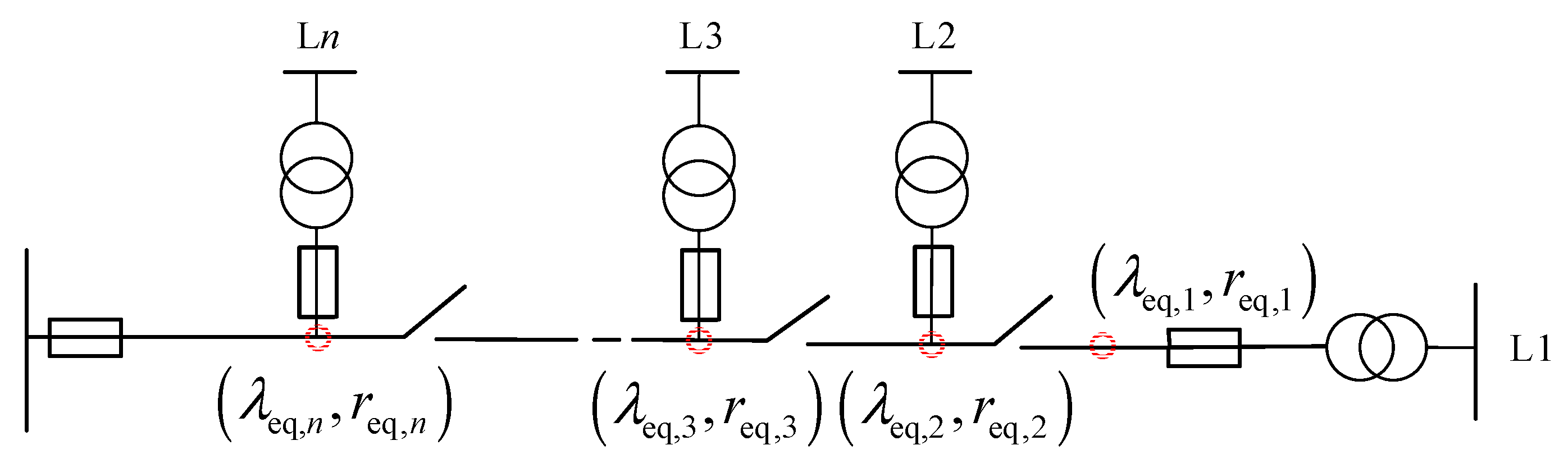
3.3.2. Equivalent to the Branch Upward of the Sectional Switch Rejection
When a section switch is at the head of a feeder branch, all s section switches in the upstream branch can break the connection between the fault area and the main distribution feeder after a fault at any point. When the segmented switch nearest to the upstream of the fault area cannot successfully isolate the fault, the fault will expand to the upstream area of the distribution network up to the head [26]. As shown in Figure 3, the branch circuit is divided into n areas according to the sectional switches, numbered from the end branch. When a fault occurs, the sectional switch in the fault area will first act to isolate the fault, and if it cannot act effectively, the upstream sectional switches will try to isolate the fault in turn under the command of the control center. Therefore, the equivalent fault rate of the distribution branch with a section switch at the first end is
where is the equivalent fault rate of the region; is the probability of effective operation of segment switch ; and is the number of segment switches.
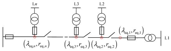
Figure 3.
Schematic diagram of upward equivalence of branches counting and segment switch rejection.
The average duration of outage in the downstream area of a segment switch is the segment switch action time if that switch can successfully operate to isolate the fault. Otherwise, the segment switches upstream of the fault operate sequentially until they spread to the branch circuit breaker. The equivalent average outage duration for a distribution branch with a sectional switch at the first end is
where is the average outage duration in the area downstream of the segment switch ; is the fault rate of segment switch ; is the equivalent fault rate of element of the branch where segment switch is located or downstream of branch ; and is the equivalent average outage duration in the area downstream of segment switch .
3.4. Calculation of User Reliability Parameters
3.4.1. General User Reliability Calculation
Ordinary users can only supply power through the main power supply of the distribution network and cannot restore a power supply through a load transfer, so the shortest path between ordinary users and the power supply is directly obtained using the minimum path method, and the impact of non-minimum path components on their reliability is discounted [27]. Thus, the failure rate and average outage time for user in scenario are
where is the number of non-minimum path branches of user ; is the number of components on the minimum path of user ; is the equivalent failure rate of non-minimum path branch of user in scenario ; is the failure rate of component on the minimum path of user in scenario ; is the equivalent average outage duration of non-minimum path branch of user in scenario ; and is the average outage duration of component on the minimum path of user n in scenario .
3.4.2. Transferable to User Reliability Calculation
- The Intentional Island User
For user n in the intentional island, the outage user has a probability to restore power through the intentional island in the scenario. Therefore, the failures in the region can be divided into internal and external by region and the failure rate of the intentional island user n in scenario c is
where is the number of components and branches on the minimum path to the main power supply in the intentional island ; is the equivalent failure rate of the component or branch on the minimum path to the main power supply in the intentional island in scenario ; and is the equivalent failure rate at user to PCC.
Therefore, the average duration of outage for the intentional island user in scenario is
where is the island operation mode switching time; is the average outage duration of element or branch on the minimum path to the main power supply in the intentional island in scenario ; and is the equivalent average outage duration at user to the PCC.
- Contact line to supply users
For the user in the transfer area of the contact line, there is a probability that the outage user can restore power through the contact line in scenario . Therefore, the failure rate of the user in this region in scenario is
where is the number of elements and branches on the smallest road to the main power supply in the diversion area of contact line i; is the equivalent fault rate of element or branch on the smallest road to the main power supply in the diversion area of contact line under scenario c; and is the equivalent fault rate at the segment switch at the first end of the diversion area of user to the contact line under scenario c.
Therefore, the average outage duration for user in the contact line under scenario is
where is the contact line switchover time; is the equivalent average outage duration of element or branch in the contact line switchover area to the main power minimum in scenario c; and is the equivalent average outage duration from user to the segment switch at the first end of the contact line switchover area in scenario c.
3.5. Reliability Calculation Process
In summary, the specific steps of the distribution network reliability calculation process based on the dynamic failure rate model of equipment in this paper are
- Initialize the parameters of each algorithm and obtain the source–load rate timing data in the time scale to be calculated based on the distribution network timing simulation model, as well as the equipment dynamic failure rate model. Input the component parameters and network structure of the distribution network.
- The source–load-rate timing data are input into the SSA-Kmeans method to obtain a typical scenario of the source–load-rate.
- Enter the probability of effective operation of segment switches, contact switches, and PCC switches.
- For the components on the non-minimum path, the equivalent fault rate and the equivalent average outage duration are calculated for each branch using the upward network equivalence method to the switch at the first end of the branch.
- Determine the type of user based on the user’s region.
- Calculate the reliability index of a typical scenario for an average user as well as the probability of contact line transfer and the probability of island formation.
- Calculate the reliability index of users in the divertable area for a scenario.
- According to the full probability formula, calculate the integrated reliability index of this system within the calculated time scale.
4. Case Studies
In order to verify the rationality of the established model and the validity of the computational methods in this paper, the calculation example was analyzed by improving the IEEE RBTS-Bus 6 feeder F4 in conjunction with the studied content. The environment of case studies is Windows10 and the processing software is MATLAB 2016a. Figure A1 is the distribution network topology diagram. Table A1 is the distribution network line data. Table A2 is the system load data. Table A3 is the distributed generation parameters. Table A4 is the component failure rate and repair time. This paper will be based on the above data for the analysis of arithmetic examples.
4.1. Analysis of Equipment Dynamic Failure Rate Results
4.1.1. Improved Age-Reduction Model
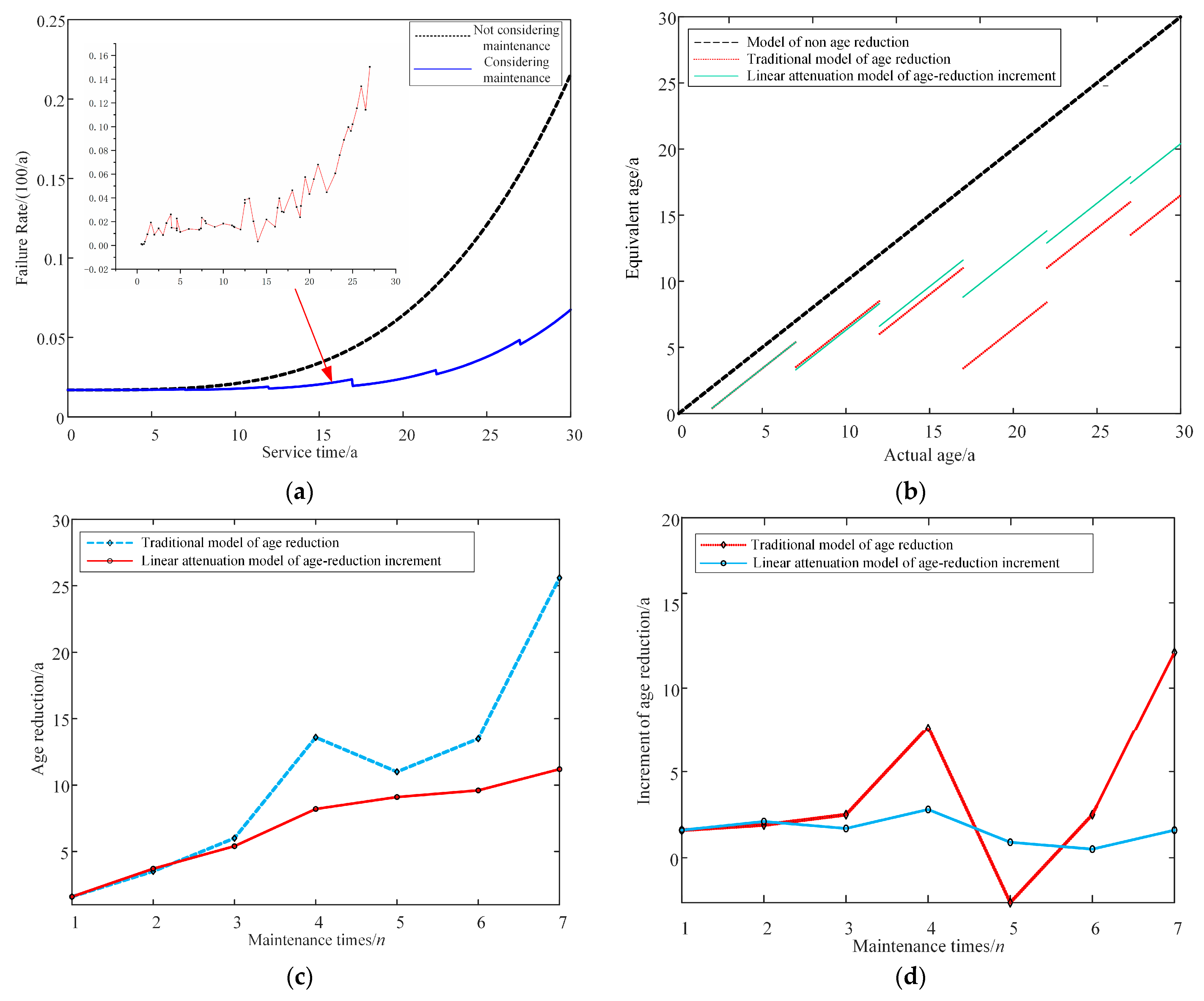
Simulation with a regional transformer to verify the correctness of the improved age-reduction model proposed in this paper. Figure 4a is the curve of the transformer failure rate. Figure 4b is retirement of service age after equipment overhaul. Figure 4c is the trend of equipment service age return with an increasing number of overhauls. Figure 4d is the trend of the increment of equipment service age retreat with the increase in the number of overhauls.
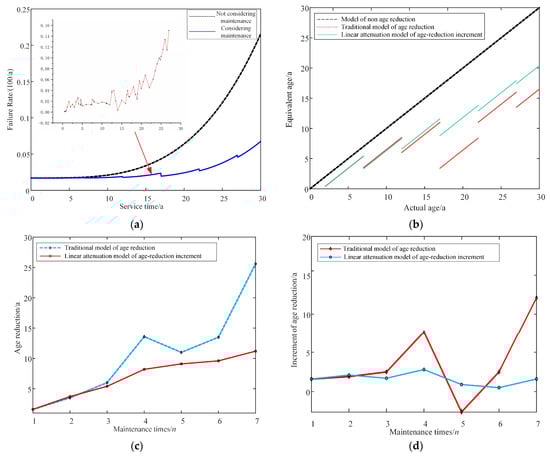
Figure 4.
(a) The curve of transformer failure rate; (b) Retirement of service age after equipment overhaul; (c) The trend of equipment service age return with an increasing number of overhauls; (d) The trend of the increment of equipment service age retreat with the increase of the number of overhauls.
As can be seen in Figure 4a, the actual equipment failure rate fluctuates upward, indicating that maintenance can increase the equipment’s condition life. But it cannot return to the initial state completely. Depending on the type of overhaul and the value of , the amount of age reduction is also different. The blue curve and the red curve will be the same if the overhaul period is the same and all the influencing factors are taken into account.
In Figure 4b, it can be seen that both the modified before and after models can well characterize the age-reduction of the device. However, the improved model can better show that the age-reduction of the equipment gradually decreases with the increase in the number of equipment overhauls. Compared with the original model, the new model is more consistent with the repair fatigue phenomenon that occurs in actual use.
Figure 4c depicts the increase in the service age setback with the number of overhauls for the new model as the number of equipment overhauls increases. However, the trend is slow and finally reaches the maximum number of overhauls tends to be constant. The service age regression increment decreases for the same type of overhaul and the increase occurs when a major overhaul is performed in that year. The incremental amount of setbacks increases relative to minor overhauls, but the overall trend is still decreasing. Therefore, the service age model with linear decay characteristics established in this paper is consistent with the actual equipment failure situation.
4.1.2. Dynamic Failure Rate of Exposed Equipment
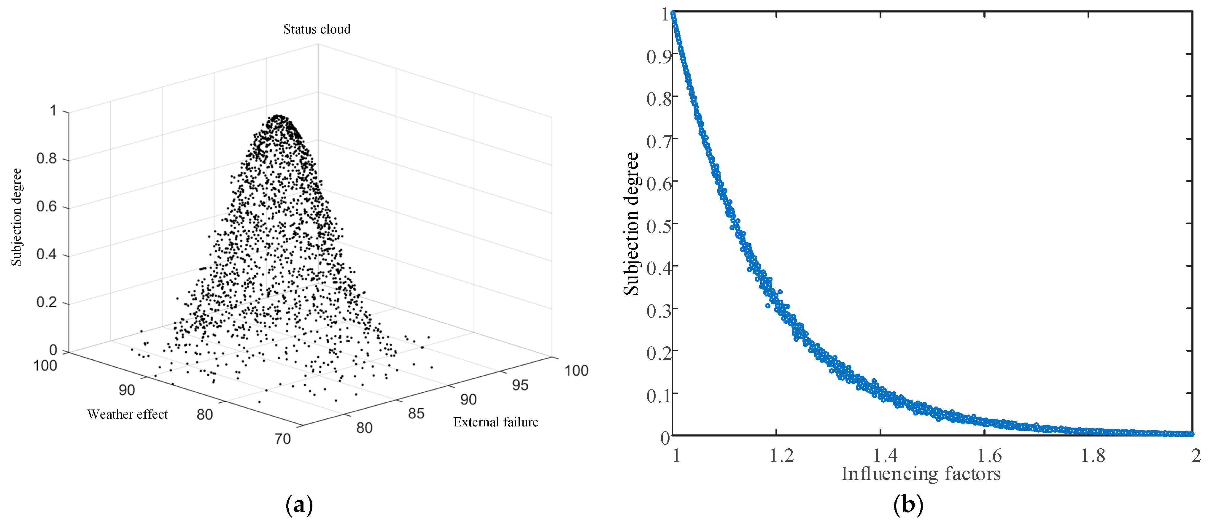
In this paper, the line history data is selected as the input of the two-dimensional normal cloud model, and the cloud droplet distribution is obtained as shown in Figure 5a. It can be seen that the two-dimensional initial cloud can better describe the uncertainty and probability distribution characteristics of the original cloud droplet. The entropy of the cloud model is calculated according to the expression of the expectation equation of Γ cloud and the super entropy is chosen as 0.05. The affiliation obtained from the two-dimensional state cloud is used as input to obtain the one-dimensional influence factor cloud. Figure 5b shows the scatter diagram of the cloud droplet composition obtained from the Γ half-drop cloud model, and the value of the influence factor increases with the increase of bad weather and the degree of external damage.
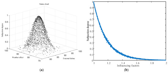
Figure 5.
(a) Two-dimensional state cloud distribution map; (b) The droplet diagram of Γ half-drop cloud model simulation cloud.
Based on the data set, the equivalent service age of the line was calculated as an input for the equivalent operating life. The optimal parameters were fitted using the L-M method, as shown in Table 2.
Table 2.
Fitting results of Line parameter (times/(10 km·a).
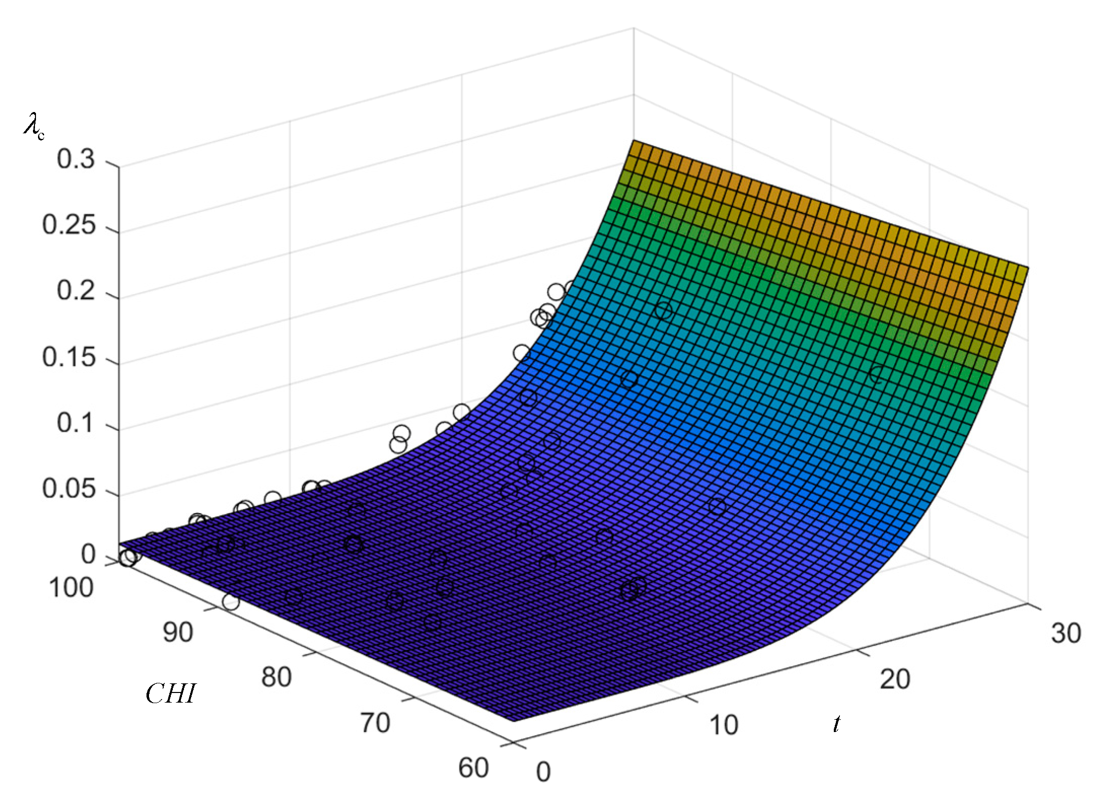
The fitted surface is plotted as shown in Figure 6 and it can be seen that the data samples are basically located on the fitted surface. In the integrated impact factor dimension, the failure rate function satisfies the trend of increasing impact factor and increasing rising slope. In the time dimension, it increases with the increase of equivalent operation years, and the failure rate rises exponentially when both the integrated influence sub and equivalent operation years are larger, which is consistent with the actual situation.
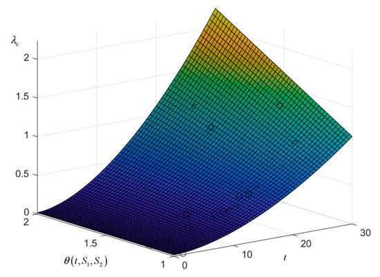
Figure 6.
The model surface of the failure rate of exposed equipment.
4.1.3. Dynamic Failure Rate of Closed Equipment
Using 56 transformers in a region [23], various influencing factors were calculated based on historically recorded data. The results of the parameters are shown in Table 3.
Table 3.
Fitting results of parameter (times/(10 km·a).
The fitted surface is plotted as shown in Figure 7 and it can be seen that the data samples are located on the fitted surface or evenly distributed on both sides of the surface. Analysis of the surface shows that at the same CHI, the failure rate is proportional to the operation time, and the transformer failure rate curve satisfies the trend that the rising slope increases with the deepening of aging; at the same aging level, the failure rate rises slowly with the decline of CHI, which is close to the actual operation.

Figure 7.
The model surface of the failure rate of closed equipment.
4.2. Scene Analysis
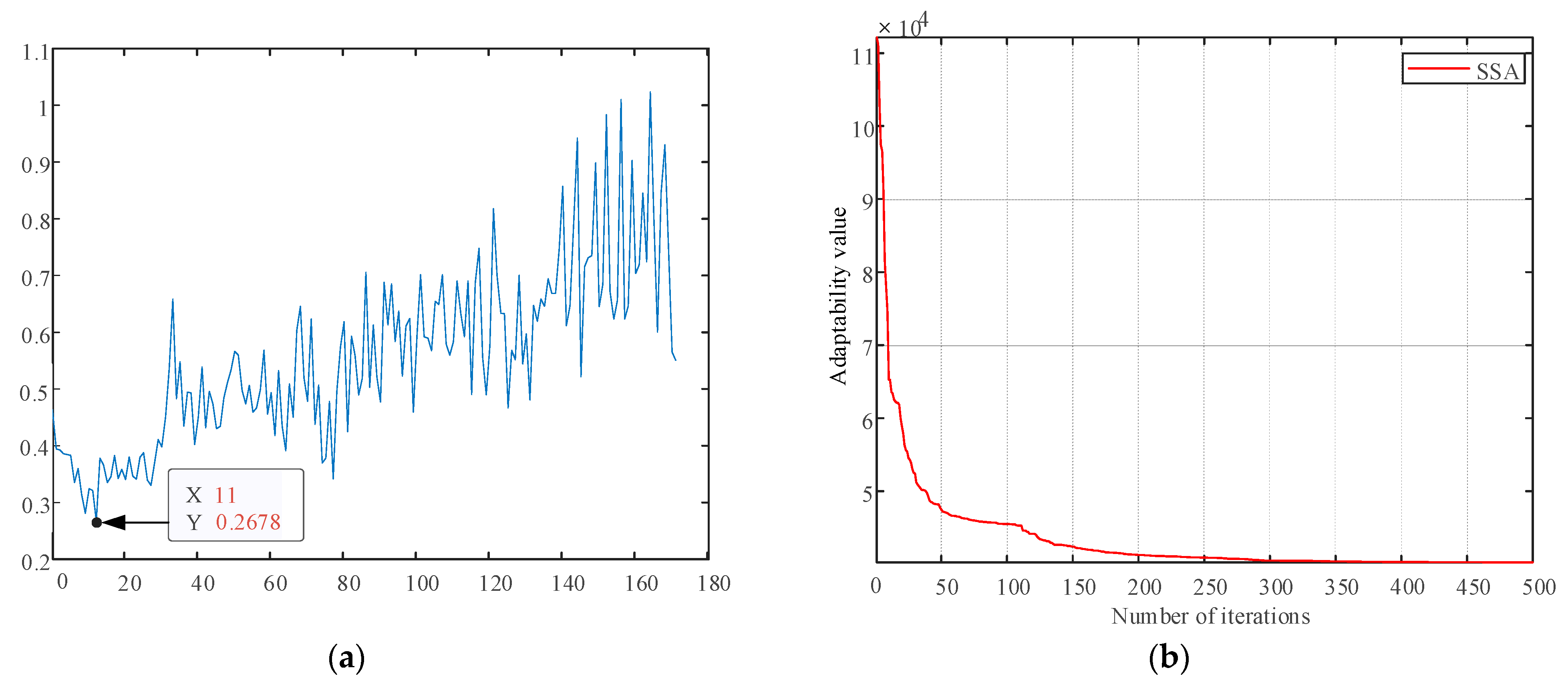
In order to reflect the source–load uncertainties as well as the time-series nature and the dynamic nature of the equipment failure rates, this paper first uses the Weibull distribution model to simulate the wind speed data of a coastal area and the Beta distribution model to simulate its light intensity, and after sampling the respective output is calculated according to the output model. Then, this paper uses the SSA-K-means method to generate typical scenarios of the source–load-rate. In order to illustrate the variability of failure rates for different devices and the same device, two different transformers and lines are selected for this study, and failure rate samples are generated according to the calculation method of failure rates presented in this paper. In the sparrow search algorithm proposed in this paper, the population size is 100, the maximum number of iterations is 500, the safety threshold (ST) is 0.8, the discoverers account for 20% of the population size, and the vigilantes account for 10%. The calculated Validity(k) curve is shown in Figure 8, and the optimal number of typical scenario classifications is 11. Therefore, the reliability indexes are calculated by dividing the distributed power output, load, and failure rate into 11 typical scenarios, and the final system reliability index values are derived. Meanwhile, to illustrate the necessity of the sparrow search algorithm to optimize K-means, the minimum value of Vadility(k) corresponding to the optimal number of scenarios before and after the comparison and the required number of iterations are shown in Table 4.
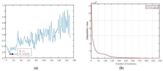
Figure 8.
(a) Validity index curve; (b) Sparrow optimizes K-means iterative curves.
Table 4.
K-means optimization before and after comparison.
As can be seen from Table 4, the optimization makes the initial clustering center selected properly, reducing the steps and times of iterative calculation, and the Validity(k) is also reduced, while the traditional K-means uses the method of randomly selecting the initial clustering center, the clustering results are more sensitive to isolated points and easily fall into local optimal solutions, and it is found that different initial clustering centers are prone to obtain a different clustering after executing the procedure several times. The clustering results of each execution are unstable. Overall, SSA-K-means can better deal with the problem of initial clustering centers and have a better clustering effect.
The distributed power output, total system load, and failure rate for each typical scenario are shown in Table 5. Figure 9 shows the probability of each typical scenario. There are no extreme cases where the probability of a particular scenario is extremely low or extremely high, indicating that the scenario extraction in this paper is reasonable.
Table 5.
Typical scenarios and probability distributions.
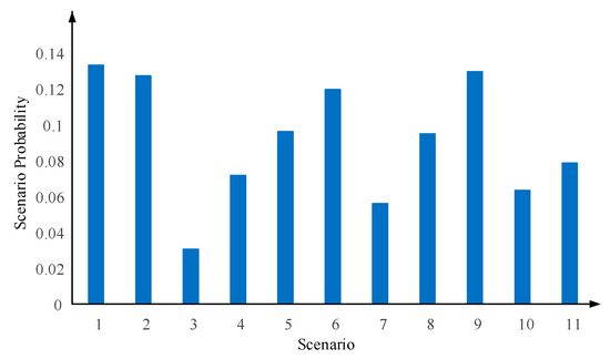
Figure 9.
Probability of occurrence of each typical scenario.
4.3. Algorithm Accuracy and Speed Analysis
In order to verify the accuracy of the reliability calculation method based on the dynamic failure rate of the equipment proposed in this paper and the efficiency of the calculation, the results of this paper are compared with the improved sequential Monte Carlo simulation method proposed in Ref. [28] to verify.
- Model 1: Methodology of this article.
- Model 2: Simulation method.
It can be visualized from Table 6 that the reliability obtained using the calculation method in this paper is different from the remaining two cases and the results are more severe. The inclusion of the time-varying failure rate in the reliability calculation increases the consideration of risk factors that can adversely affect the system and better reflects the actual system power supply level. Compared with the constant failure rate method, a large value will result in conservative calculation results, which will cause a waste of human and financial resources, while a small failure rate will overestimate the power supply level of the distribution network to a certain extent and prevent the timely detection of potential system failures. The method in this paper is closer to the actual situation of the system, which is beneficial to the safe operation of the grid.
Table 6.
Distribution network reliability index under two methods.
It can be seen that the results calculated by the two methods are similar, with a difference of 6.32% for SAIFI, 6.29% for SAIDI, 0.33% for CAIDI, 0.01% for ASAI, and 2.31% for EENS, and the difference between the reliability indexes calculated by the two methods is not significant when the calculation errors are ignored. Therefore, the calculation method proposed in this paper has certain accuracy, and the proposed calculation idea of considering the source load and the time-series correlation of failure rate has certain feasibility.
In terms of computation time, the total computation time of the simulation method is about 72.76 times that of this paper. In order to ensure the convergence of the algorithm itself and the accuracy of the computation results, the sequential Monte Carlo method requires large-scale random simulation, and the computation time is sacrificed to meet the computation accuracy. Therefore, the method of this paper can save computation time and the algorithm has certain high efficiency under the premise that the reliability index of the system can be shown comprehensively, and the uncertainty of random variables can be simulated effectively.
4.4. Reliability Calculation Based on Time-Varying Failure Rate Model
In this paper, a dynamic failure rate model of the equipment is developed. In order to represent the impact of dynamic failure rate on the reliability of the distribution network, taking the modified microgrid as an example [23], the modeling scheme of the calculation is as follows.
- Model 1: The failure rate is a constant model without consideration of source–load-rate temporality.
- Model 2: The equipment failure rate considers a typical scenario of source–load-rate but the failure rate is constant.
- Model 3: The failure rate model proposed in this paper.
4.5. Analysis of the Impact of Load Transferable Supply
There are three main types of customers studied, including general types of customers, customers who can be diverted through the intentional island and customers who can be diverted through contact lines. The ability to transfer loads reflects the high degree of automation in the distribution system and is used to analyze the impact of load transferability on the reliability level of the distribution network.
4.5.1. Transfer of Supply through Intentional Island
- Model 1: The distribution network contains no intentional islands.
- Model 2: The distribution network contains intentional islands, but the effective operation efficiency of energy storage, DG, and PCC switches is not considered and only the offline island formation probability is considered.
- Model 3: The distribution network contains intentional island, and the effective operation probability of each element is considered, i.e., the calculation method in this paper.
As can be seen from Table 7, the reliability of loads outside the intentional island is not affected by the intentional island. Comparing Model 1 and Model 2, from the perspective of system reliability, SAIFI is reduced by 8.878%, SAIDI by 9.787%, CAIDI by 0.999%, ASAI by 0.04%, and EENS by 22.093%; therefore, the use of planned island can effectively improve the reliability of the distribution network.
Table 7.
Reliability index results in different cases.
Comparing Model 2 and Model 3, the SAIFI increases by 1.639%, SAIDI by 1.828%, CAIDI by 0.184%, ASAI is almost unchanged, and EENS by 4.778%, so the successful operation of the planned silos depends on the scheduling of the control center in centralized control and is slightly less reliable compared to local control independent of communication.
4.5.2. Transfer of Supply through Liaison Lines
- Model 1: There is no contact line in the distribution network.
- Model 2: There are contact lines in the distribution network but the probability that the contact lines can form a diversion channel is not considered.
- Model 3: There are contact lines in the distribution network and the probability that the contact lines can form a transfer channel is considered, which is the calculation method in this paper.
- Model 4: On the basis of Model 3, the maximum transfer of the contact line is set to 12 MW.
- Model 5: On the basis of Model 3, the maximum diversion of the contact line is set to 1 MW.
Table 8 shows the calculation results of reliability indicators under different conditions. Comparing Model 1 and Model 2, it can be seen that SAIFI, SAIDI, CAIDI, ASAI, and EENS are reduced by 14.988%, 16.818%, 2.148%, −0.08%, and 16.38%, respectively, when the liaison line is set up, indicating that the liaison line transfer can effectively improve the reliability of the distribution network.
Table 8.
Reliability index results in different cases.
Comparing the data of Model 2 and Model 3, it can be seen that the reliability indicators of the system SAIFI, SAIDI, CAIDI, ASAI, and EENS increased by 5.653%, 6.488%, 0.784%, −0.02%, and 6.2745%, respectively, indicating that after considering whether the switch can be successfully operated, the number of user failures increased and the failure time grew, thus reducing the system reliability of the system. Therefore, the ability of the switch to receive control commands and act correctly has an impact on the calculation of system reliability and cannot be ignored.
Comparing Models 3, 4, and 5, it can be seen that when the maximum transmission power of the contact line is within a certain range, increasing the maximum power of the contact line has a positive effect on the system reliability but when the maximum transmission power increases to a certain degree, the impact on the reliability is slight. Therefore, in actual operation, the maximum transmission power of the contact line should be selected while ensuring reliability and taking into account the economy.
In summary, the distribution network reliability calculation based on the dynamic failure rate of equipment can more closely simulate the actual operation of the grid, mainly in the correct modeling of the equipment failure rate, which decreases the distribution network reliability after considering each risk factor and can more accurately characterize the reliability on the statistical time scale, so that the reliability calculation is no longer limited to the long-term steady state.
5. Conclusions
In the background of large-scale renewable energy access and the close connection of information and communication networks to the distribution network, the active distribution network is developing rapidly, and the need for more accurate and faster reliability calculations for the active distribution network has arisen. This paper investigates the multivariate dynamic failure rate modeling of equipment and the fast reliability calculation method for the uncertainty of source–load under information failure. The main findings and conclusions of this paper are as follows:
(1) Dynamic failure rate model for two types of equipment is constructed based on fuzzy theory and data-driven methods. Based on the case study, the model is verified to avoid the lag and subjectivity of failure rate calculation. At the same time, it is more suitable for engineering practice and can be adapted to long-term and short-term predictions.
(2) An improved SSA-K-means algorithm is adopted for the temporality and correlation among the source, load, and failure rate. The method optimizes the clustering effect of the scenes, improves computational accuracy, and avoids local optimum. The cases show that the method can achieve a better classification result and obtain a more rational classification with fewer iterations.
(3) Based on the consideration of island operation and contact line transfer, a fast reliability calculation method that takes into account the uncertainty and computational efficiency in the distribution network is proposed in combination with the improved minimum path method, which is suitable for reliability calculation on multi-time scales. The calculation time of this method is reduced by 72.76 times compared to the traditional method. It is verified that the method can take into account uncertainty and risk factors and guarantee the accuracy of reliability calculations while taking a better account of economics. This provides the reference indicators for the optimal dispatch of active distribution networks.
Future work in this direction can further build a multi-state fault model based on the two-state fault model and consider the modeling of information transmission performance by taking into account the switch timing method to form more refined modeling in the case of multi-energy flow coupling.
Author Contributions
Conceptualization, Z.L., J.L. and T.Z.; methodology, J.L. and T.Z.; software, J.L., T.Z. and J.S.; validation, Z.L. and J.L.; formal analysis, J.L., T.Z. and J.S.; investigation, J.L. and T.Z.; resources, J.L. and T.Z.; data curation, J.S.; writing—original draft preparation, Z.L., J.L., T.Z. and J.S.; writing—review and editing, Z.L. and J.L.; visualization, J.L. and T.Z.; supervision, Z.L.; project administration, Z.L. All authors have read and agreed to the published version of the manuscript.
Funding
This research was funded by the National Natural Science Foundation of China. Project name: Research on general modeling and multi-system collaborative planning of integrated energy system. Grant number No. 51977074.
Data Availability Statement
Date not available to be shared.
Conflicts of Interest
The funders had no role in the design of the study; in the collection, analyzes, or interpretation of data; in the writing of the manuscript; or in the decision to publish the results.
Appendix A
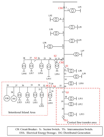
Figure A1.
Distribution network topology diagram.
Figure A1.
Distribution network topology diagram.
Table A1.
Distribution network line data.
Table A1.
Distribution network line data.
| Number | Length (km) | Number | Length (km) |
|---|---|---|---|
| 1 | 2.8 | 16 | 2.8 |
| 2 | 2.5 | 17 | 3.2 |
| 3 | 1.6 | 18 | 2.5 |
| 4 | 0.9 | 19 | 3.2 |
| 5 | 1.6 | 20 | 1.6 |
| 6 | 2.5 | 21 | 0.8 |
| 7 | 0.6 | 22 | 2.8 |
| 8 | 1.6 | 23 | 2.5 |
| 9 | 0.75 | 24 | 3.2 |
| 10 | 0.9 | 25 | 2.8 |
| 11 | 3.2 | 26 | 2.5 |
| 12 | 2.8 | 27 | 0.75 |
| 13 | 0.6 | 28 | 1.6 |
| 14 | 3.5 | 29 | 3.2 |
| 15 | 1.6 | 30 | 2.8 |
Table A2.
System load data.
Table A2.
System load data.
| Number | Number of Users | Load Size/MW | Load Classification |
|---|---|---|---|
| 1, 6 | 147 | 1.90 | Second class load |
| 2 | 126 | 1.81 | Third class load |
| 3, 13, 17 | 1 | 1.54 | Third class load |
| 4, 18 | 1 | 1.15 | Third class load |
| 5 | 132 | 1.12 | First class load |
| 7, 23 | 1 | 1.48 | First class load |
| 8, 11, 14, 19 | 79 | 1.63 | Third class load |
| 9, 21 | 1 | 1.80 | First class load |
| 10, 12, 16, 22 | 76 | 1.09 | Second class load |
| 15, 20 | 1 | 1.27 | Second class load |
Table A3.
Distributed Generation parameters.
Table A3.
Distributed Generation parameters.
| Type | Parameters | Value |
|---|---|---|
| Wind power generation | Rated power | 0.3 MW |
| Rated wind speed | 12 m/s | |
| Cut-in wind speed | 3 m/s | |
| Cut-out wind speed | 24 m/s | |
| Photovoltaic power | Rated power | 200 × 0.0002 MW |
| Standard light intensity | 1 km/m2 | |
| Standard working temperature | 25 °C | |
| Power temperature coefficient | −0.0045 |
Table A4.
Component failure rate and repair time.
Table A4.
Component failure rate and repair time.
| Type | Failure Rate λ (Time/a) | Repair Time r (h) |
|---|---|---|
| Circuit Breaker | 0.002 | 4 |
| Transformer | Dynamic models | 200 |
| Line | Dynamic models | 4 |
| Section switch | 0.05 | 8 |
| Interconnection switch | 0.015 | 200 |
| DG | 0.3 | 20 |
| ESS | 0.5 | 10 |
| PCC | 0.05 | 8 |
Table A5.
Abbreviations Cross Reference.
Table A5.
Abbreviations Cross Reference.
| Abbreviations | Complete Formulation |
|---|---|
| DG | Distributed Generation |
| ESS | Electrical Energy Storage |
| PHM | Proportional Hazard Model |
| HI | Health Index |
| CHI | Comprehensive Health Index |
| PV | Photovoltaic |
| SSA | Sparrow Search Algorithm |
| PCC | Point of Common Coupling |
| ST | Safety Threshold |
| RMSE | Root Mean Square Error |
| R | Correlation Coefficient |
| SAIFI | System Average Interruption Frequency Index |
| SAIDI | System Average Interruption Duration Index |
| CAIDI | Customer Average Interruption Duration Index |
| ASAI | Average Service Availability Index |
| EENS | Expected Energy Not Supplied |
References
- Fan, M. Active power distribution system definition and research. Distrib. Util. 2015, 171, 45–47. [Google Scholar] [CrossRef]
- Ma, G. Research on Risk Assessment Method of Power Grid Considering Ime-Varying Failure Rate of Overhead Lines; Zhengjiang University: Hangzhou, China, 2020. [Google Scholar]
- Li, Z.; Wang, F.; Guo, W.; Mi, Y.; Ji, L. Resilience Evaluation of Smart Distribution Network in Extreme Weather. Autom. Electr. Power Syst. 2020, 44, 60–68. [Google Scholar]
- Jing, L.; Chen, L.; Zhao, D.; Luo, Y. The Study of Overhead Line Fault Probability Model Based on Fuzzy Theory. Energy Power Eng. 2013, 5, 625–629. [Google Scholar]
- Zhang, G.; Zhang, J.; Peng, Q.; Duan, M. Index System and Methods for Power Grid Security Assessment. Power Syst. Technol. 2009, 33, 30–34. [Google Scholar]
- Yang, J.; Liu, P.; Hu, W.; Wu, W.; Yu, T. Method for predicting failure rate of power transmission equipment based on cloud theory. High Volt. Eng. 2014, 40, 2321–2327. [Google Scholar] [CrossRef]
- Song, W.; Wen, W.; Guo, Q.; Chen, H.; Zhao, J. Performance evaluation of sensor information fusion system based on cloud theory and fuzzy pattern recognition. In Proceedings of the 2020 IEEE International Conference on Information Technology, Big Data and Artificial Intelligence (ICIBA), Chongqing, China, 6–8 November 2020; pp. 299–303. [Google Scholar]
- Ma, Z.; Shang, Y.; Yuan, H.; Shi, S.; Sheng, W.; Huang, R.; Shen, P. Holistic performance evaluation framework: Power distribution network health index. IET Gener. Transm. Distrib. 2017, 11, 2184–2193. [Google Scholar] [CrossRef]
- Zheng, J.; Hu, C.; Si, X.; Zhang, Z.; Zhang, X. Remaining useful life estimation for nonlinear stochastic degrading systems with uncertain measurement and unit-to-unit variability. Acta Autom. Sin. 2017, 43, 259–270. [Google Scholar] [CrossRef]
- Nakagawa, T. Sequential imperfect preventive maintenance policies. Reliab. IEEE Trans. 1988, 37, 295–298. [Google Scholar] [CrossRef]
- Gu, J.; Du, J.; Qin, J.; Zhang, Y. A Fuzzy Programming Model Basedon Life Cycle Cost for Equipment Maintenance in Substations. Autom. Electr. Power Syst. 2014, 38, 7. [Google Scholar]
- Guo, Q.; Xin, S.; Wang, J.; Sun, H. Comprehensive Security Assessment for a Cyber Physical Energy System: A Lesson from Ukraine’s Blackout. Autom. Electr. Power Syst. 2016, 40, 145–147. [Google Scholar]
- Yan, T.; Tang, W.; Wang, Y.; Zhang, X.; Xu, S. Reliability Evaluation of Distribution Network With Microgrid Based on Multi-State Energy Storage Model. Power Syst. Technol. 2017, 41, 2222–2228. [Google Scholar] [CrossRef]
- Tang, W.; Yan, T.; Wang, Y.; Zhang, X. Reliability Evaluation of Distribution Network Containing Microgrids Based on Multi-State Power Interruption Sequence Model. Power Syst. Technol. 2019, 43, 285–293. [Google Scholar] [CrossRef]
- Cheng, L.; Wan, Y.; Qi, N.; Tian, L. Review and Prospect of Research on Operation Reliability of Power Distribution and ConsumptionSystem Considering Various Distributed Energy Resource. Autom. Electr. Power Syst. 2021, 45, 191–207. [Google Scholar]
- Li, G.; Huang, Y.; Bie, Z.; Ding, T. Machine-learning-based reliability evaluation framework for power distribution networks. IET Gener. Transm. Distrib. 2020, 14, 2282–2291. [Google Scholar] [CrossRef]
- Cox, D.R. Regression Models and Life-Tables (With Discussion). J. R. Stat. Soc. Ser. B (Stat. Methodol.) 1971, 34, 187–220. [Google Scholar]
- Xiong, S. Research on Risk Control of Power Grid Operation Considering Transmission and Transformation Equipment Factors; Zhejiang University: Hangzhou, China, 2016. [Google Scholar]
- Zhang, K.; Chen, J.; Guo, C.; Fan, C.; Zhang, J.; Deng, M. Weather Factor Based Analysis on Probabilistic Load Flow of Power Grid Containing Wind Farms. Power Syst. Technol. 2014, 38, 3418–3423. [Google Scholar] [CrossRef]
- Xiong, X.; Wang, W.; Yu, Y.; Shen, Z.; Cheng, R.; Dai, Z. Risk Analysis Method for Transmission Line Combining of Various Meteorological Factors. Proc. CSU-EPSA 2011, 23, 11–15+28. [Google Scholar]
- Espinoza, S.; Panteli, M.; Mancarella, P.; Rudnick, H. Multi-phase assessment and adaptation of power systems resilience to natural hazards. Electr. Power Syst. Res. 2016, 136, 352–361. [Google Scholar] [CrossRef]
- Hu, Y. Analysis and Prevention of Transmission Line Operation Fault. China Electr. Power Press 2007, 1–8. [Google Scholar] [CrossRef]
- Zhou, Y. Research on Transformer Operation and Maintenance Strategy and Economic Life Based on Health State; North China Electric Power University: Beijing, China, 2019. [Google Scholar]
- Tang, A.; Han, T.; Xu, D.; Xie, L. Path planning method of unmanned aerial vehicle based on chaos sparrow search algorithm. J. Comput. Appl. 2021, 41, 2128–2136. [Google Scholar]
- Kapourchali, M.H.; Sepehry, M.; Aravinthan, V. Fault Detector and Switch Placement in Cyber-Enabled Power Distribution Network. IEEE Trans. Smart Grid 2018, 9, 980–992. [Google Scholar] [CrossRef]
- Liu, W.; Lin, Z.; Ma, T.; Wang, Z.; Gong, Q. Reliability Modeling and Evaluation of Active Distribution System Considering Effect of Cyber Invalidity. Autom. Eletr. Power Syst. 2019, 43, 94–102. [Google Scholar]
- Liu, Z.; Zhang, T. Failure Probability Model of Distribution Network Equipment Based on Improved Age-Reduction Model and Factor Correction. In Proceedings of the 2021 IEEE/IAS Industrial and Commercial Power System Asia (I&CPS Asia), Chengdu, China, 18–21 July 2021; pp. 639–645. [Google Scholar]
- Wang, Z. Micro-Grid Reliability Calculation Method Study Considering the Time Relevance and the Component Operation Hours; North China Electric Power University: Beijing, China, 2018. [Google Scholar]


Disclaimer/Publisher’s Note: The statements, opinions and data contained in all publications are solely those of the individual author(s) and contributor(s) and not of MDPI and/or the editor(s). MDPI and/or the editor(s) disclaim responsibility for any injury to people or property resulting from any ideas, methods, instructions or products referred to in the content. |
© 2023 by the authors. Licensee MDPI, Basel, Switzerland. This article is an open access article distributed under the terms and conditions of the Creative Commons Attribution (CC BY) license (https://creativecommons.org/licenses/by/4.0/).