1. Introduction
Access to energy carriers is a key issue for the functioning of a stable economy. When demand varies, supply must be balanced. In the case of natural gas, underground gas storage facilities are used to balance demand and supply discrepancies. During the warm months, when there is no need for household heating, the surplus supply of natural gas is used to fill underground storage volumes. It makes stable gas production from domestic reservoirs and undisturbed (on the recipient’s side) import of contracted gas volumes possible. Then, during winter (or colder months), when gas demand exceeds supply, storage facilities are switched to withdrawal mode, and the stored gas fills the gap between (too low) supply and (increased) demand [
1].
Storage facilities are also used to buffer daily peak demands and prevent the disruption of supply during mechanical issues or other problems in the producing fields [
2,
3]. Gas in UGS is divided into two parts: working (or active) gas and cushion gas. Working gas is the amount of gas that can be withdrawn and injected during one cycle of UGS operation. Critical to the operation of gas storage reservoirs is the use of cushion gas, i.e., gas that compresses and expands as the working gas is injected and withdrawn but that is not produced itself. Cushion gas is most commonly leftover native gas in the reservoir; if the amount of gas left in the reservoir is less than that required for cushion, it has to be injected. However, inert cushion gas, such as nitrogen (
), is injected to substitute natural gas in the cushion of UGS facilities [
4,
5]. Gas storage facilities are common around the world, and there are many guidelines for selecting a site [
3], creating storage facilities, and studies related to the description and analysis of various issues related to gas storage [
6].
Carbon dioxide capture, use, and storage (CCUS) are together accepted as one of the options to mitigate anthropogenic carbon dioxide emissions, thus contributing to the stabilization of atmospheric greenhouse-gas concentrations [
7]. Geological storage of
has the potential to significantly decrease emissions in a relatively short period of time. There is great interest in the issue of
capture and storage (CCS), which results in many studies, analyses [
8,
9,
10], and guidelines [
11,
12]. Numerical simulation, widely accepted in the petroleum industry as a standard forecasting tool, has been adopted for the simulation of geological storage of
, including storage capacity assessment and risk characterization, among others [
5,
13,
14]. The concept of combining geological storage of carbon dioxide with underground storage of natural gas is interesting but not well-investigated. Oldenburg [
5] analyzed the use of
as cushion gas and justified it with the high effective compressibility of
, near its critical pressure, and economic purposes. He pointed out the differences between methane and carbon dioxide as cushion gas and presented the results of numerical simulations performed on a simplified horizontal model that incorporated a single well and was initially filled with
or
. On the basis of the results obtained, he concluded that the use of
as cushion gas is possible and promising. According to [
15], gas storage with
as cushion gas may also be a logical choice for the further development of gas reservoirs that have been filled with
during carbon sequestration combined with enhanced gas recovery (CSEGR).
Lingyu Mu et al. [
14] analyzed the use of
as cushion gas using a numerical model that consists of an element of the symmetry of the horizontal layer initially filled with water. Injection of carbon dioxide and methane, and gas withdrawal are carried out with the same well. The model represents a closed system; therefore, an additional well is used to mitigate the increase in pressure during the injection phase by producing brine out of the pore volume. The authors highlighted the following advantages of using
as cushion gas:
Carbon dioxide in reservoir conditions exists in two basic forms, pure in a supercritical state or mixing gas with , both of which are quite different from the working gas;
Pure and its mixtures with methane have higher compressibility than , which results in more space for the working gas;
The density of pure is much higher than that of within the operating pressure range of UGS; the great difference in density results in stratification relying on gravity;
is more viscous than .
In [
14], the authors investigated the effect of porosity, permeability, production rate, and time on
content in withdrawn gas. Based on the results obtained, they concluded that the dissolution of
in brine should be included when modeling the interaction between
and
in the pore medium; higher porosity causes a slight decrease in
content in the produced gas, and the higher the permeability, the higher the content of
. Although the work of the authors provides a better understanding of the dynamics of UGS supported by the
cushion, it covers only one injection/withdrawal cycle.
Considering that (1) gas storage reservoirs are generally high-permeability clastics or carbonates (1000–10,000 mD in situ permeability in common) existing at intermediate depths and temperatures [
3], (2) there exists the aforementioned significant influence of permeability on
content in the produced gas, and (3) cyclic injection and withdrawal must influence the behavior of the system, detailed and comprehensive analysis is needed.
In this study, we used a more realistic anticline-shaped model instead of a simple horizontal “shoes-box” model and injection of out of the target working-gas pore volume. Injecting with the use of the well that is used to operate storage (injection and withdrawal of natural gas)—as in the presented studies—has the obvious advantage of limiting the number of wells but simultaneously causes the risk of developing an extensive mixing zone in the stage of storage development and limits the potential storage capacity. Therefore, we propose not to inject directly into the center of the storage zone but rather at a distance. Injecting at a distance from the UGS operating wells appears to take advantage of the -based cushion on one hand and limit the effect of mixing between methane and carbon dioxide within storage on the other hand. These additional wells can be used to monitor storage and/or to convert storage to storage in the future.
In our approach, an analytical aquifer was used. It enabled better representation of real gas reservoir performance with a dynamic aquifer, where brine moves in and out of the gas zone during UGS operation. We also decided that to achieve more reliable reservoir behavior, the simulation had to include a reservoir depletion period. Furthermore, the simulations performed included 10 cycles of UGS operation, which allowed us to cover the long-term effects resulting from multiple storage emptying and filling operations.
2. Materials and Methods
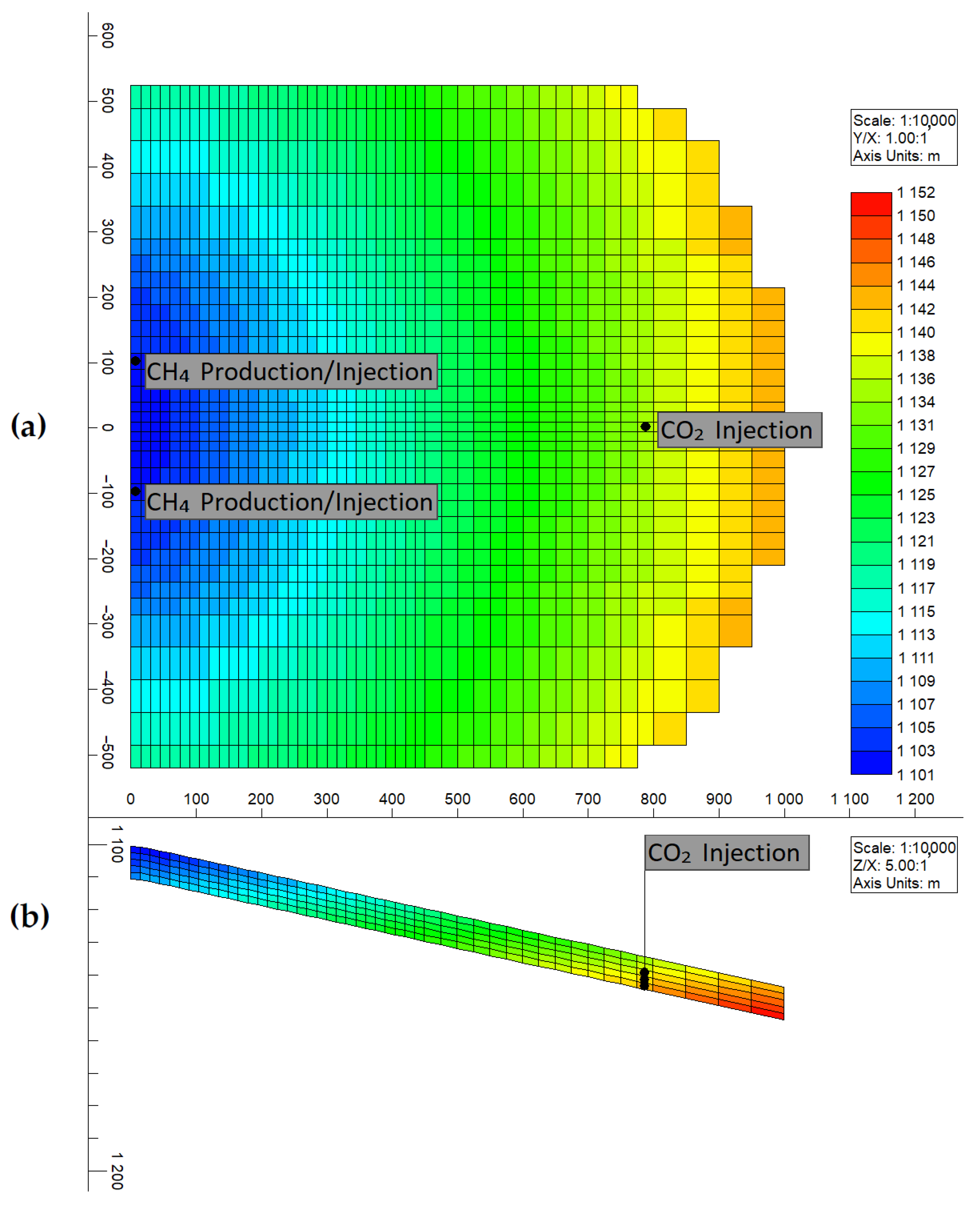
The numerical model used in this study represented half of the anticline, with a dip angle of 2.5
in the I- and J-directions. It consisted of 48, 35, and 5 blocks in the I-, J-, and Z-directions, respectively. The aerial dimensions of the model were 1000 m by 1040 m, while the model thickness was set to 10 m. The basic parameters of the model are shown in
Table 1. The aerial view and the cross section along the longest wing of the anticline and through the
injection well are shown in
Figure 1.
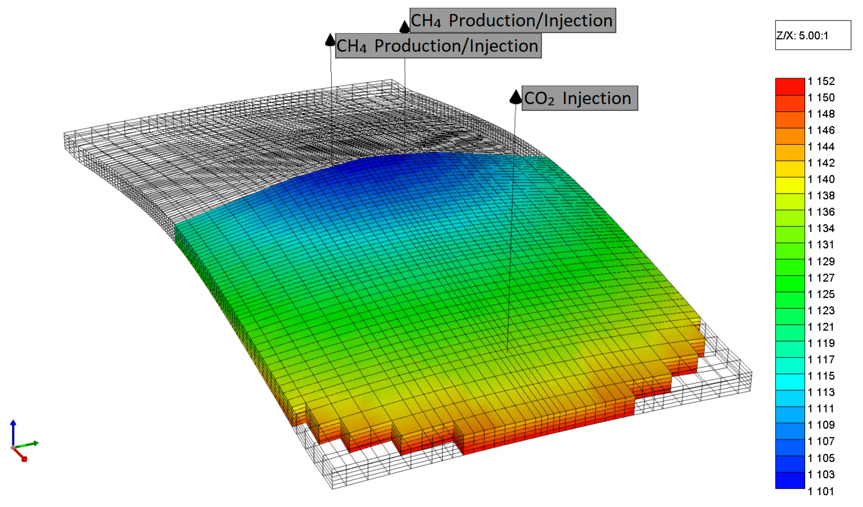
The license used in this study allowed simulations to be only carried out on models consisting of up to 10,000 blocks. For this reason, the analysis was only performed on the symmetry element of the anticline (half of the anticline). A 3D view of the whole anticline model, with the color filled part being the part that was used in further simulations, is shown in
Figure 2.
Due to the limitation on the number of blocks, the main production/injection wells, which were placed at the top of the model near the “cutting edge”, had to be specially modified. The first parameter that was changed was
wfrac. It is a real dimensionless number between 0.0 and 1.0 that specifies the fraction of a circle that the well models. Usually,
wfrac = 1.0 if the well is in the interior of the block [
16]. In this case, the wells were placed on the side of the block, so
wfrac = 0.5 for these wells was fixed. The second parameter was
geofac, which is a positive, real, dimensionless number that specifies the geometric factor for the well element. This factor depends on the placement of the well within the grid block and on the placement of the grid block relative to the boundaries of the reservoir [
16]. In this case,
geofac = 0.54 was set for these wells.
The distance between the main production/injection wells was 200 m, and the distance between them and the injection well was around 793 m for both. At the side and bottom grid edges of the model, an analytical aquifer was connected. It made it possible to maintain pressure in the reservoir without the cost of additional grid blocks. The R-Ratio equaled 10, and the modeling method was Carter–Tracy with limited extent. The CMG builder allowed us to use preset tables with dimensionless time and pressure functions.
The reservoir temperature of 40 C, which is above the critical temperature of , was assumed. Simulations were performed based on the standard assumption of isothermal conditions within the reservoir. Under these two conditions, pure only occurred in the supercritical phase or in the gaseous phase when the pressure dropped below its critical pressure. The mixture of both components ( and ) cannot condense to the liquid phase under such conditions either. The dissolution of in water was also included.
Permeability, in addition to porosity, which is responsible for a sufficient volume of storage, is a major property that allows injection and production at required delivery rates during peak demand periods. Gas storage reservoirs are generally high-permeability clastics or carbonates that exist at intermediate depths and temperatures [
3]. High permeability ensures good flow in the reservoir and well bottom-hole pressure maintenance and is thus highly desired when selecting a reservoir or aquifer for underground gas storage. However, in the case of the use of
as a part of cushion gas, it mixes with natural gas within the reservoir pore space, and high permeability, with the resulting “ease of flow”, may accelerate the movement of
towards the near-well zone. For this reason, the analysis of the effect of permeability on
content in the withdrawal gas and the overall performance of UGS seems to be of high importance.
In this study, we analyzed the effect of permeability on the operation of UGS with a part of the cushion gas replaced with
, especially with respect to
content in the gas withdrawn from storage. A single porosity value was assumed, and permeability was related to porosity by considering the pore throat aperture at 35% mercury saturation as per mercury injection capillary pressure (MICP) measurement according to [
17]. Process or delivery speed, i.e., the ratio of permeability and porosity, provides a relative indication of storage and of how quickly fluids can move through porous media and, as such, is widely used to characterize oil and gas reservoirs of various lithologies [
18,
19] and to predict recoverable hydrocarbon volumes [
20]. Pore throat aperture (
), in microns (
m), can be calculated using a correlation developed by Aguilera (2002, 2004) utilizing data on more than 2500 sandstone and carbonate samples [
17]:
Assuming that different rock types are represented by the range of values of
, a range of permeability values can be obtained by rearranging Equation (
1) with respect to permeability:
where
—pore throat aperture (
m);
k—permeability (mD); and
—porosity (%).
Underground gas storage facilities are made in deposits with
good reservoir properties, so we assumed a range of
to represent reservoir rocks with pore throat aperture classified as macropores (
(2.5–10)
m) and megapores (
> 10
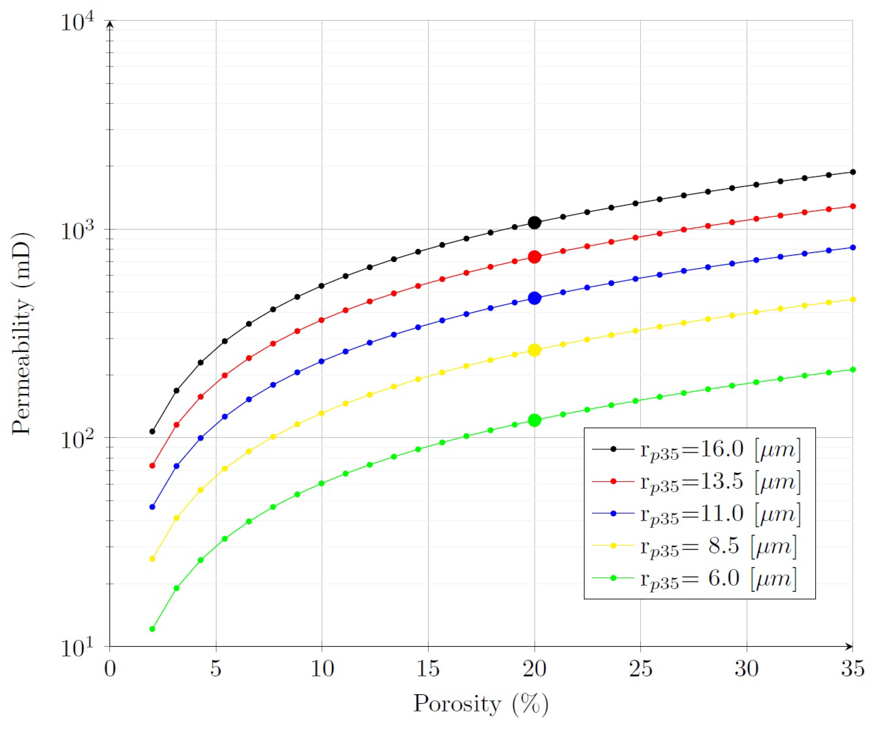
m). Five values of
were used in this study: 6.0, 8.5, 11.0, 13.5, and 16.0
m. The porosity of 20% was assumed and was fixed throughout the analysis. This porosity value is reasonable and
good enough to meet the underground gas storage requirements. Additionally, it allowed high permeability to be obtained with the use of the adopted methodology. The relationship between permeability and porosity for each assumed value of the diameter of the pore throat is shown in
Figure 3. Permeability increases with the increase in pore throat aperture. For the assumed range of
, permeability covered the range from 121 mD to 1073 mD. In the following part of the paper, the models are referred to by their
values. The permeability anisotropy of 10% was assumed.
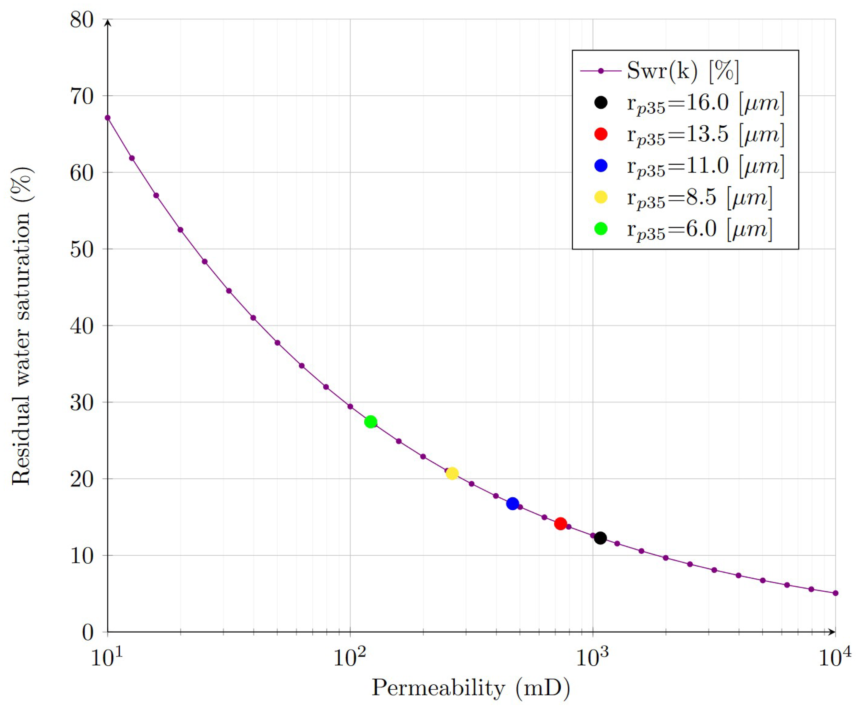
Another parameter defining reservoir rocks and directly influencing their storage capacity is connate water saturation. According to [
21], residual water saturation can be estimated based on porosity and permeability with the use of the following empirical equation:
where
—residual water saturation (%);
k—permeability (mD); and
—porosity (%).
The relation between residual water saturation and permeability for a hypothetical reservoir rock with porosity of 20% and different pore structure represented by different
values is shown in
Figure 4. Generally, the higher the permeability, the lower the residual water saturation.
In addition to its effect on storage capacity, water saturation is crucial to calculating the relative permeability values that govern the multiphase fluid flow during simulations. Herein, the relative permeability curves were separately and consistently computed for each model to capture the effects of different pore structures on the process of interest. The widely accepted Brooks–Corey model for the gas phase and the water phase, i.e., Equation (
4) and Equation (
5), respectively, was used:
where
and
—relative permeability values of gas and water;
—relative permeability of gas at connate water saturation;
—relative permeability of water at irreducible gas saturation;
and
—gas and water saturation values;
and
—critical saturation values of gas and water;
and
—connate saturation values of gas and water; and
and
—exponents for gas and water (relative permeability and saturation values are expressed as fractions of one).
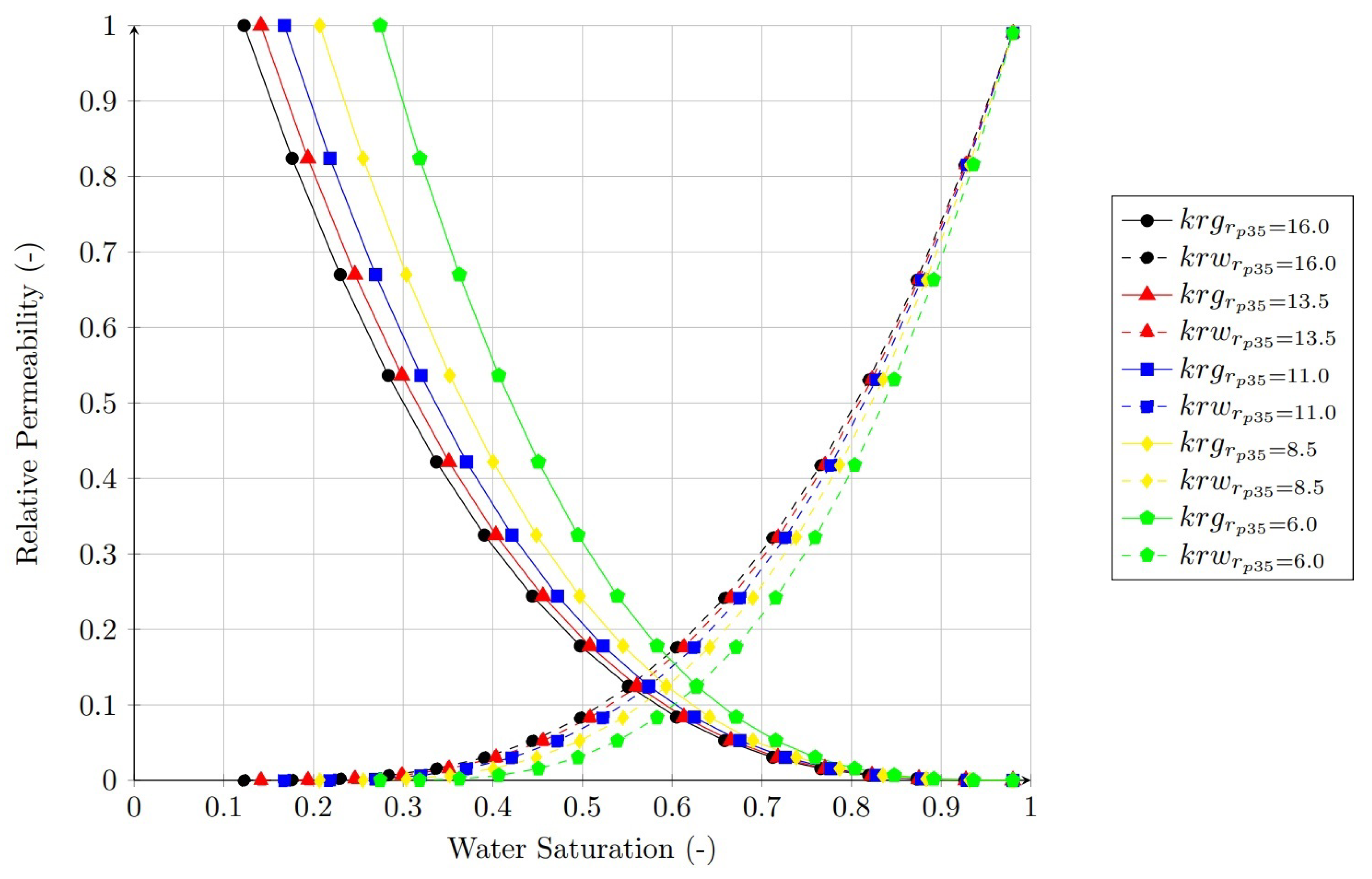
The exponents for these equations were assumed to be equal to 3, which is appropriate for well-sorted consolidated sandstone. The relative permeability curves for gas and water for each model are shown in
Figure 5. It was assumed that critical water saturation was equal to residual water saturation; the critical gas saturation of 0.02 was assumed. The reservoir parameters of all models are summarized in
Table 2.
The modeled process was carried out with the use of one injection well and two production/injection wells for half of the anticline. Due to the fact that in the CMG GEM simulator, each well can operate in one mode, as producer or injector, the UGS wells were doubled and switched on/off depending on the operating mode (withdrawal/injection).
The amounts of injected and produced gases were the same for each case analyzed. An active gas-to-cushion gas ratio of 50/50 was assumed. The goal was to replace 25% of cushion gas with
with respect to the reservoir conditions in the fully filled state. As the models were different with respect to the pore volume available to the gas phase (owing to different residual water saturation), the pore volume of the
m model was taken as a reference to calculate the amounts of natural gas and carbon dioxide that are presented in
Table 3. The mass of the injected carbon dioxide was 17.42 thousand metric tons. The reservoir pressure at full storage was assumed to be equal to the initial reservoir pressure.
The simulation comprised three distinct stages: (1) gas field depletion, (2) injection of both natural gas and , and (3) actual underground gas storage operation. In the first stage, gas production was modeled with the use of two wells, _PROD_1 and _PROD_2, and the amount of gas removed equaled the assumed volume of active gas plus 25% of cushion gas (with regard to initial reservoir conditions) to make space for carbon dioxide. This stage lasted for a year and three months. It would have been possible to skip this step and start the simulation of the model representing an already depleted reservoir; however, in this case, the pressure difference between the aquifer and the reservoir resulting from the depletion phase would not have been captured. After withdrawing, the assumed volume of the gas reservoir entered a one-month stabilization stage.
The second stage started with the injection of , which was maintained with the use of wells and and lasted five months. After the next month-long stabilization stage, the injection of started through well and continued for 11 months.
The third stage covered the main operation of gas storage. From November to March, that is, during the coldest months, when natural gas supply is lower than demand, the storage facility operated in withdrawal mode, while during the warmest months (from May to September), when natural gas supply is higher than demand, natural gas was injected into the storage facility. Each phase of UGS operation was followed by one month of stabilization (October and April).
The daily rates of gas injection and production were the same for all models and are presented in
Table 4. Both UGS wells operated at the same gas rates, and the gas rates were assumed to be constant during the withdrawal and injection periods. Rates were relatively low, but as mentioned, only half of the anticline was modeled, so in the case of the whole structure, these rates should be multiplied by a factor of two.
3. Results
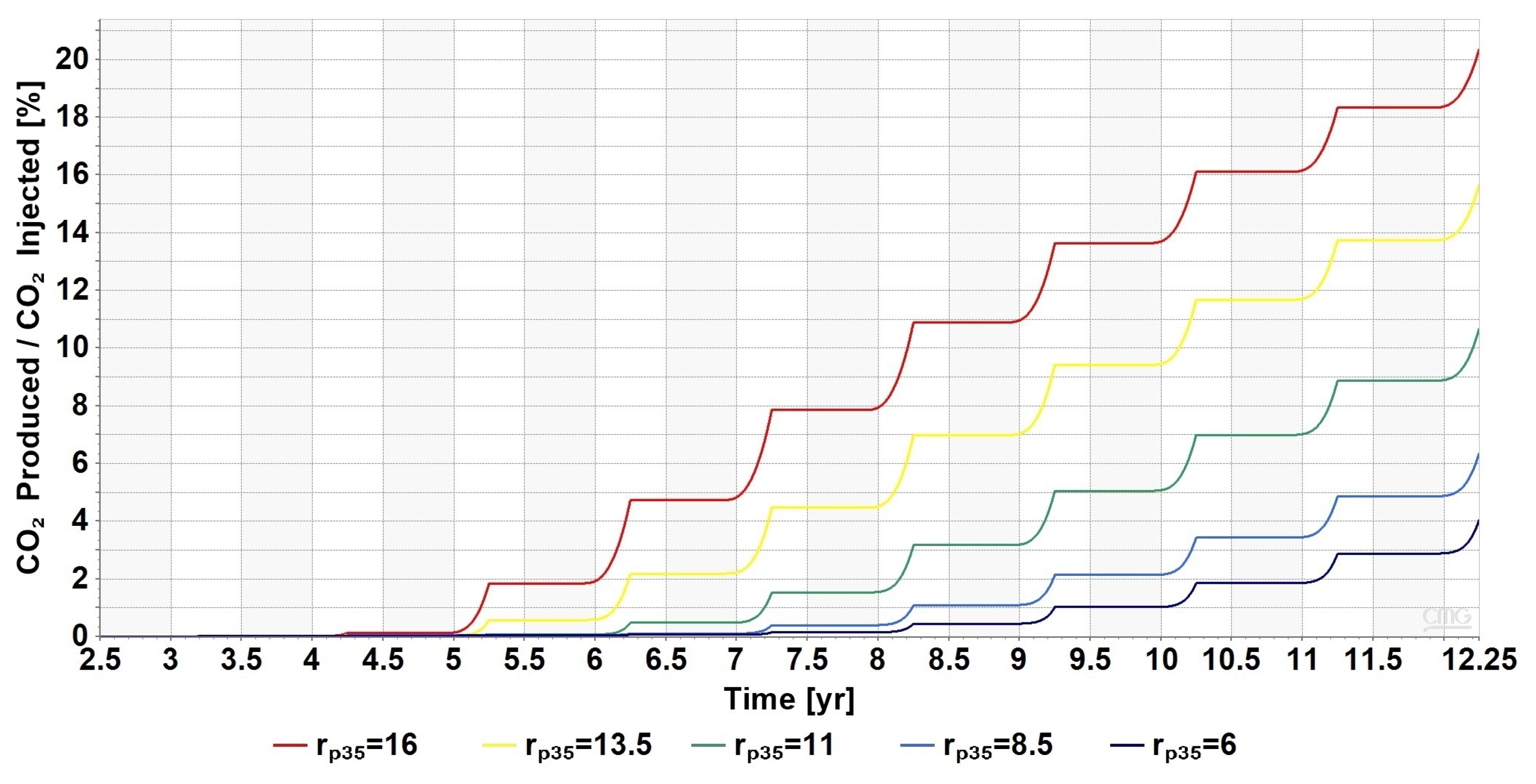
In
Figure 6, the ratios of the cumulative withdrawal of
moles from the two producing wells to the injected
moles are shown. After 10 cycles of UGS, the highest percentage of depletion of injected
moles was that of the
m model (1073 mD) and equaled 20.4%. The lower
was, the lower the percentage of depletion. The lowest was that of the
m model (121 mD) and equaled 4.1%. The exact values of this parameter in all models are shown in
Table 5.
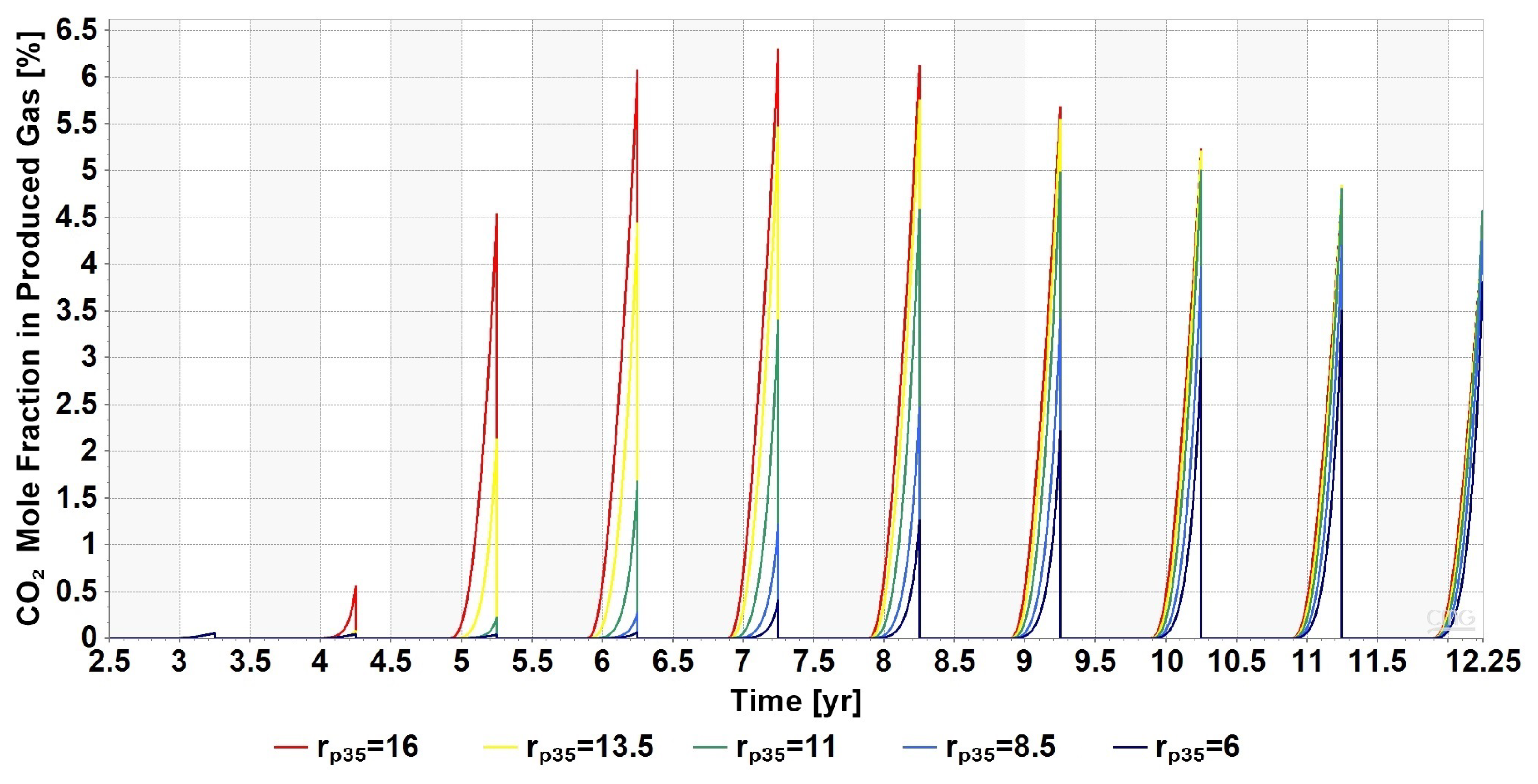
The comparison of the
mole fraction in the gas produced in all models is shown in
Figure 7. The highest values occurred at the end of the production stages in all models. From
Table 5, where the maximum values of the
mole fraction in the produced gas and the production cycle of its appearance are shown, it follows that the highest maximum value and the value that occurred the earliest among all models were those of the
m (1073 mD) model. The maximum peak value and the moment of its appearance were related to
. The lower
was, the lower the maximum value, and the more delayed the moment of its occurrence. After the maximum values of the
,
, and 11
m models, the peak values in the next production stages decreased. Regarding the
and 6
m peaks, the values only increased with successive cycles and may have been higher than the maximum reached in the 10th cycle.
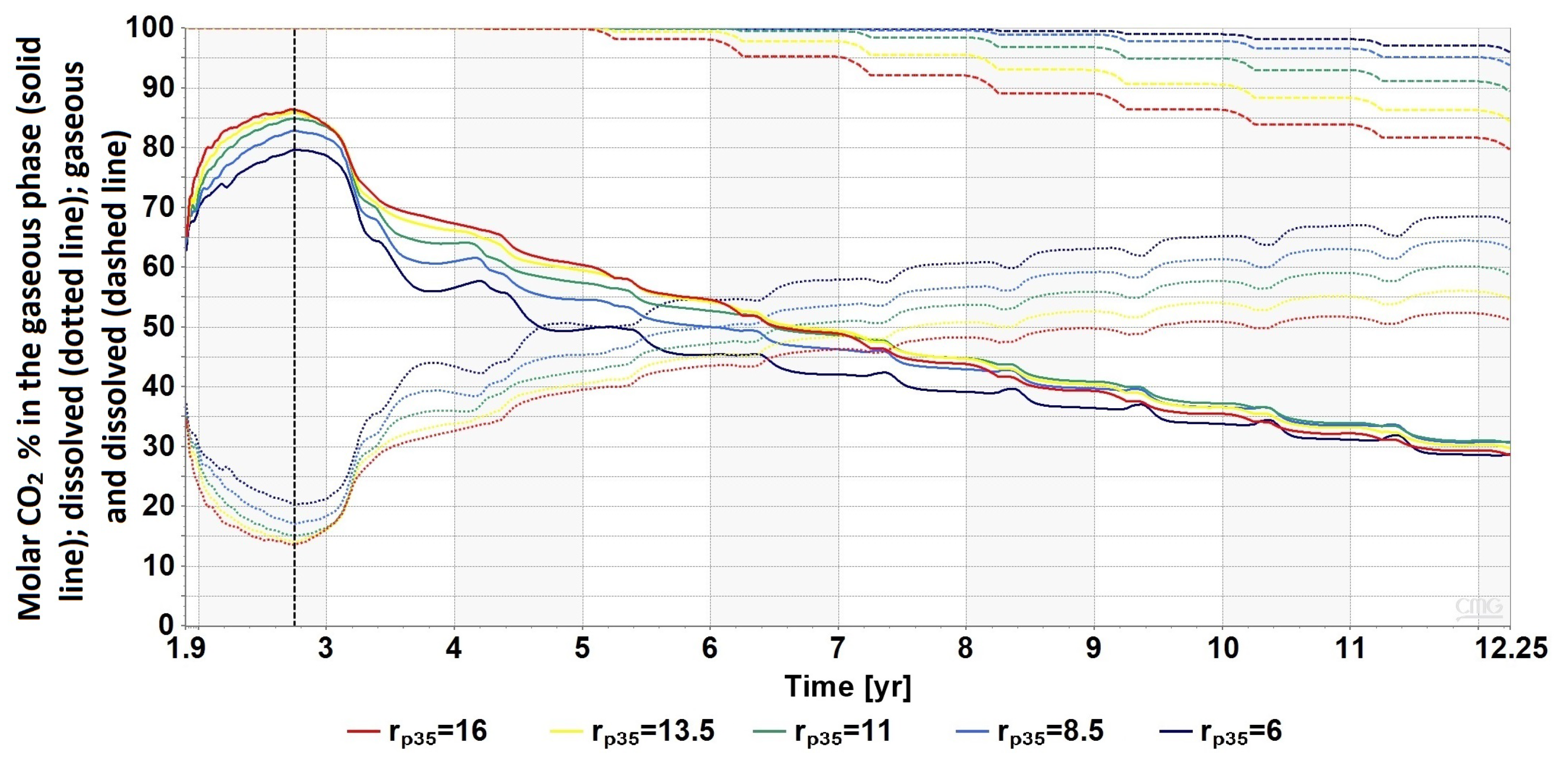
In
Figure 8, the ratios of
moles in the gaseous phase to injected
moles, and dissolved
moles to injected
moles, and their sum are shown. In the
injection stage (on the left side of the black dashed line in
Figure 8), the ratio in the gaseous phase increased, and for dissolved
, it decreased. In fact, dissolved
also increased, but those ratios were relative to the injected
moles that grew rapidly, and the dissolution did not occur fast enough. In our simulations, we did not distinguish between gaseous and supercritical
, but it is important to note that our gaseous ratio included supercritical
when the reservoir pressure was higher than the critical pressure of
(around 7.38 MPa) and gaseous
when the pressure was lower.
At the end of the
injection phase, the maximum values of
moles occurred in the gaseous phase. The highest value of the gaseous ratio was that of the
m (1073 mD) model, and the lower
was, the lower this parameter was. The exact values of all models are shown in
Table 6. At this point, the minimum value of dissolved
of all models also occurred.
After the injection of
, when the UGS facility started to work (on the right side of the black dashed line in
Figure 8), the gaseous part of
decreased, and the dissolved part increased. The growth of the dissolved
ratio was similar for all the models, and the highest value was found with
m; the higher
was, the lower this ratio was. The decrease in the gaseous phase ratio was greater for models with higher
because this phase was simultaneously dissolved and withdrawn (decrease in the sum of the dissolved and gaseous ratios in
Figure 8). Due to the higher withdrawal of
in models with higher
, the decrease in the gaseous phase ratio was also higher. The values of the dissolved and the gaseous
ratios at the end of the 10th production cycle are also shown in
Table 6.
After the first few UGS cycles, where the changes were abrupt, during the injection stage, the dissolved mostly grew; during the production stage, the changes were not significant; and during stabilization after production (when the average pressure was low), the dissolved decreased. This is because dissolution is pressure-dependent, and the higher the pressure, the higher the dissolution.
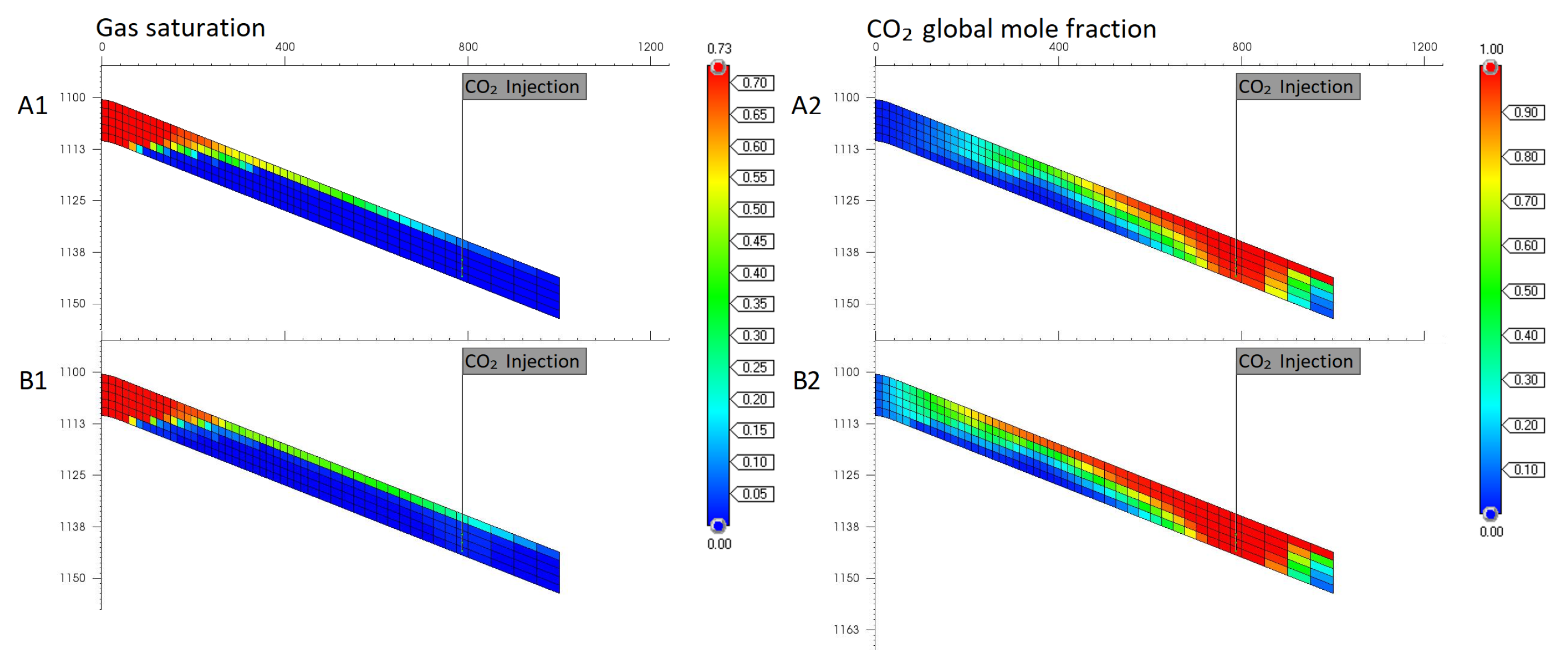
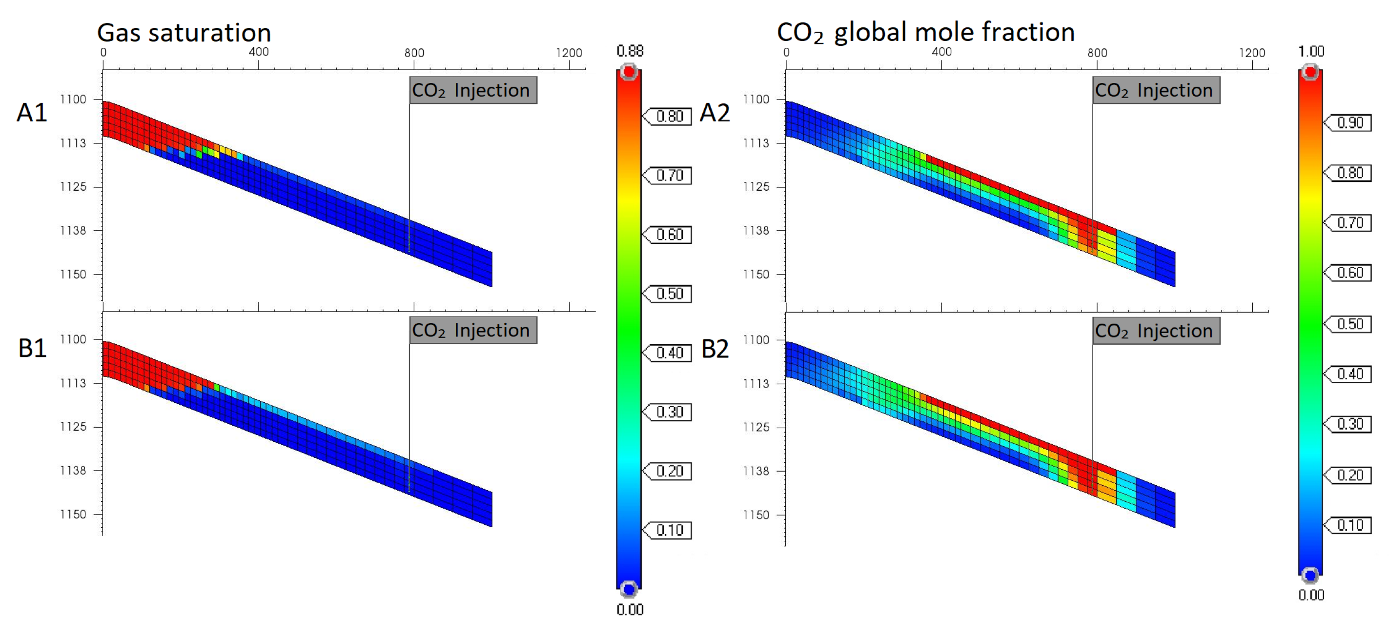
Cross sections through the center of the model that represent gas saturation and
global mole fraction before and after the 10th production cycle of the
m and
m models are shown in
Figure 9 and
Figure 10, respectively. It follows from them that
in the gaseous phase was mainly in the roof layer, and in lower parts, there was only dissolved
(which was included in the
global mole fraction). For this reason, the analysis of the
distribution in the models was carried out on the aerial views of the models.
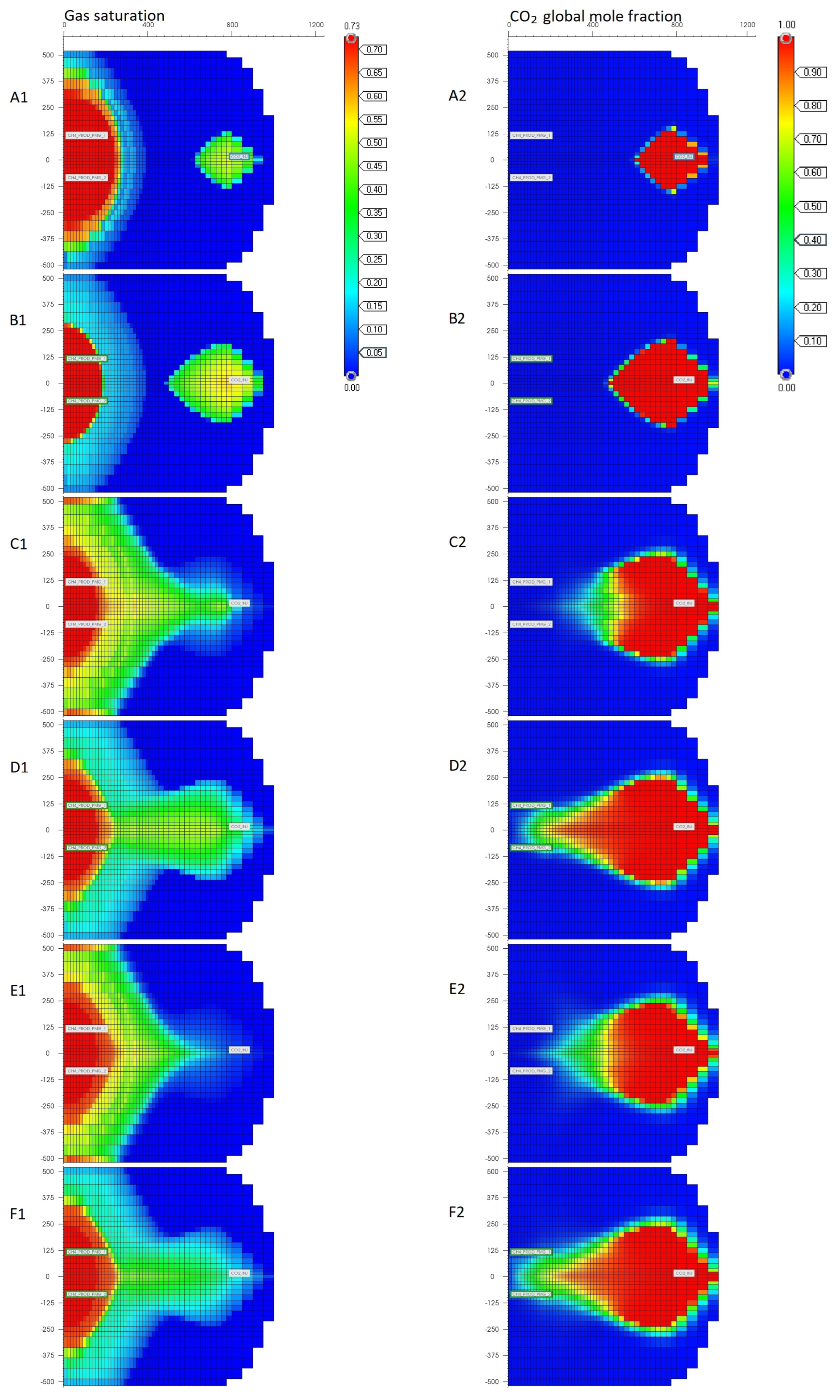
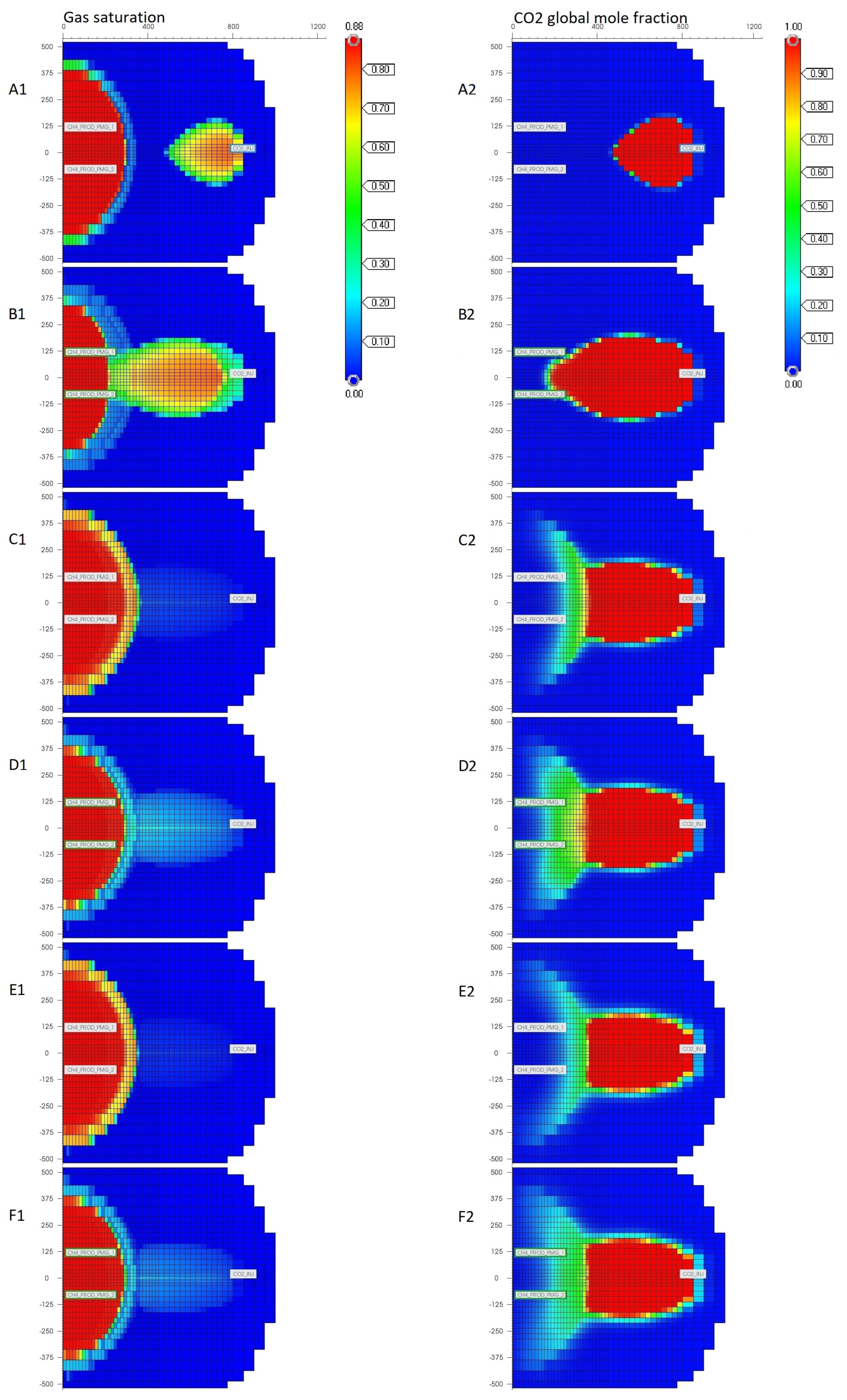
Aerial views of gas saturation and
fraction in gas before and after the first, sixth, and tenth production cycles of the
m (121 mD) and
m (1073 mD) models are represented in
Figure 11 and
Figure 12, respectively.
Before the first production cycle, the injected did not reach the methane area in either case. In the aerial view of model with higher , the gas-saturated area in place of injection was wider than that in model with lower permeability. This was due to higher vertical permeability, which caused faster movement of from lower layers. After the first production cycle in the case of the m model, still did not reach the methane area, in contrast to m, at which reached methane, but the aerial view of the fraction indicated that mixing did not start.
Before the sixth production cycle in the m model, was connected to and mixed with the methane area, but the blocks where mixing took place were relatively far from the operating wells and little gas-saturated. In the case of the m model, approximately all was in the initial methane area. There was a noticeable difference in the shape of propagation and mixing. At m, there were still gas-saturated blocks in the injection area, and the path of movement to the methane area was clearly outlined. Mixing occurred in this relatively narrow path. In the m model, widespread mixing occurred in the lower parts of the methane area. After the sixth production cycle in the case of the m model, the “movement path” width of the gas-saturated blocks increased. In the methane area, gas saturation decreased the most in the lower parts. was much closer to the operating wells than before production. In the m model, approached the UGS operation wells.
Before the 10th production cycle in the m model case, the gas from the injection area was still moving to the methane area. After the 10th production cycle, the situation was similar to that of the 6th cycle. In the case of the m model, the situation during the whole 10th cycle was similar to that during the 6th cycle.
The gas area in the
m model during 10 cycles of UGS operation did not stabilize, and the movement of
did not end. In the
m model, the gas area stabilized much faster and was highly gas-saturated and compact. Clearly visible from
Figure 11 and
Figure 12 are differences in
propagation patterns. High permeability (thus high vertical permeability) ensured fast migration of
to the methane area and mixing along the lower border of it. Lower permeability (thus lower vertical permeability) prevented fast migration and mixing and forced
to move linearly in the operating well direction.
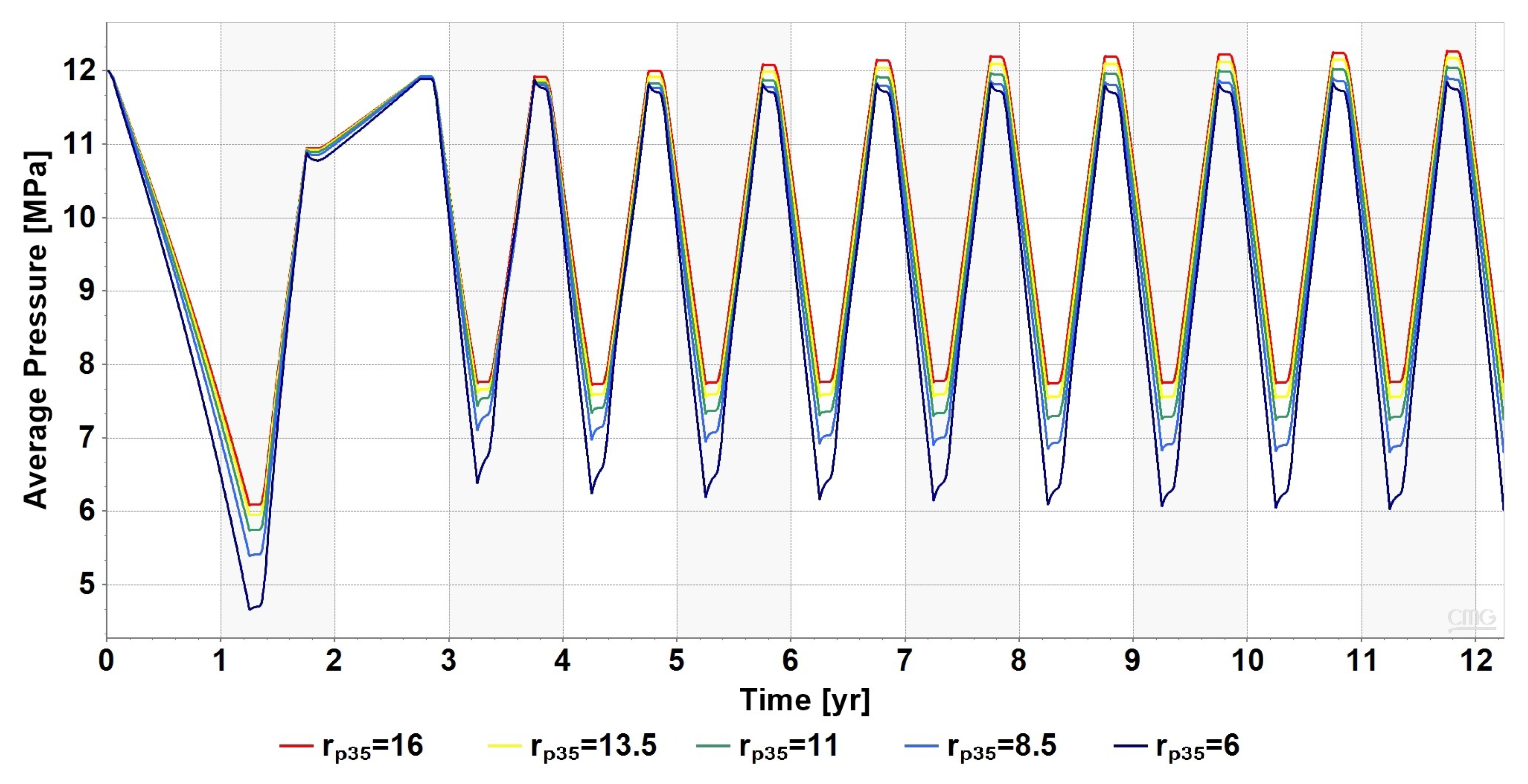
In
Figure 13, the comparison of the average pressure in all models is shown. The average pressure is relative to
, which affects permeability and, as a result, changes the pore volume available to hydrocarbons (different connate water saturation). In all steps, the highest average pressure was that in the
m (1073 mD) model. The lower
was (thus the lower the pore volume available to hydrocarbons was), the lower the average pressure was. The differences were more significant at the end of the production period and increased with successive cycles (1.36 MPa in the first cycle and 1.76 MPa in the last cycle). At the end of the injection period, the differences were smaller (approximately 0 MPa before the first cycle and 0.42 MPa in the last cycle).
It was noticeable that the pressure when the storage was full increased with successive cycles. The largest growth (when comparing the pressure at the end of injection) was that in the m model, and the changes were smaller with lower (at r = 16 m, the model difference for 10 cycles equaled 0.35 Mpa; in the r = 6 m model, this was almost 0 MPa). This was due to the replacement of with , which is less compressible. The higher the depletion, the lower the compressibility of the system, and the higher the average pressure. This may partly explain the increasing differences described in the previous paragraph.
In all models, during the stabilization phase, the average pressure grew after the production phase and decreased after the injection phase. The difference was that the magnitude of this pressure growth/drop was dependent on . The highest magnitude of growth/drop was observed at m (121 mD) and was lower at higher . Higher (thus permeability) provided better flow from the aquifer to the model, which ensured faster pressure equalization.
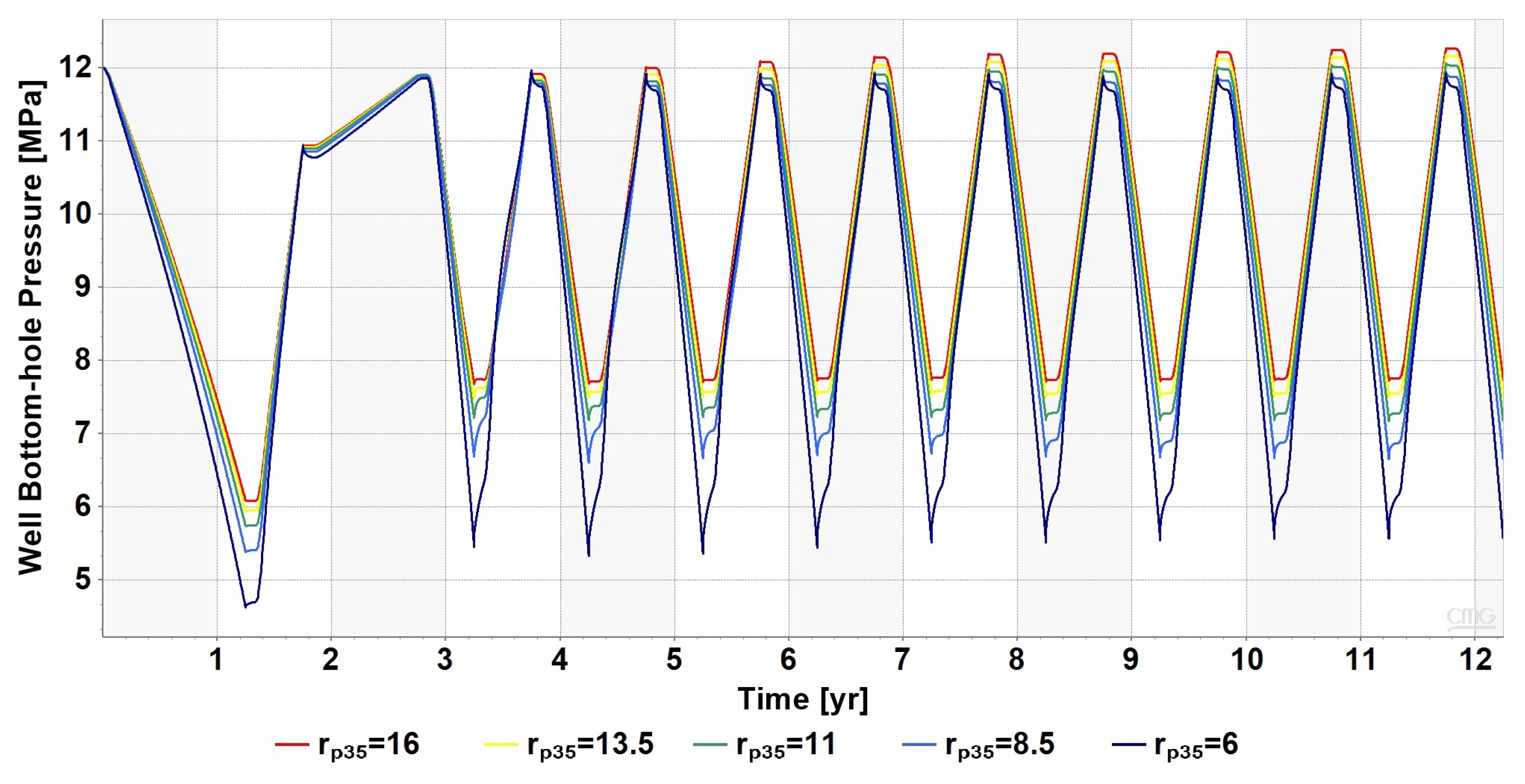
In
Figure 14, the comparison of the bottom-hole pressure is shown for all models. As in the case of the average pressure, the highest bottom-hole pressure in all steps was that in the
m (1073 mD) model and was lower when
was lower (thus lower permeability). The absolute differences between the average pressure and the bottom-hole pressure were the biggest at
m (121 mD) and the lowest at
m. The peak value occurred at the end of the production phases, and the maximum value occurred in the first cycle (at
m, 0.95 MPa; at
m, 0.08 MPa) and decreased with successive cycles.
4. Discussion
We studied the behavior of underground gas storage with cushion gas partially substituted with carbon dioxide in five different lithologies represented by the range of the radius of the pore throat. At fixed porosity, the effect of permeability determined based on the methodology was evaluated in terms of content in withdrawn gas and the general withdrawal of injected .
Having the same porosity, models with different pore structures differed with respect to permeability, covering the range from 121 mD to 1073 mD. Moreover, the resulting differences in initial water saturation and thus in the pore volume available to natural gas (and/or carbon dioxide) were incorporated. These differences affected the models’ pressure behavior with regard to the average reservoir pressure and well bottom-hole pressure.
Underground natural gas storage operates in yearly cycles of withdrawal and injection. This is a dynamic system where not only gas but also brine (in the case of active aquifers) flows in and out of the storage trap. When in the cushion is considered, the behavior of the system is significantly more complex.
Our results show that the permeability of reservoir rocks has a great influence on content in withdrawal gas. In the model with the highest permeability (1073 mD), after 10 cycles of UGS operation, 20.4% of injected was produced back to the surface. In the case of the model with the lowest permeability analyzed (121 mD), this ratio was only 4.1%. High permeability accelerates the process of migration of toward operational wells and mixing with stored natural gas.
In our analysis, we assumed that the same amount of gas (with respect to volume under normal conditions) was produced/injected in each model. The higher the permeability of the model, the more and less methane were produced in subsequent cycles. Therefore, after each injection phase, the total amount of methane (compared with ) increased, changing the compressibility of the system. In other words, the withdrawn was replaced with methane, which is less compressible. For this reason, in models with higher (higher permeability), the average pressure increased with successive cycles. Permeability also has a significant effect on bottom-hole pressure. High permeability ensures better bottom-hole pressure maintenance.
Our results show the evolution of the propagation and mixing zone over ten consecutive cycles, and significant differences among models with different pore structures were observed. In the model with the lowest permeability, the flow of within the reservoir seemed to be mainly driven by the pressure gradients caused by storage operations (withdrawal and injection). The mixing zone was relatively compact and limited in area. With the growth in permeability, buoyancy-driven flow effects appeared: the mixing zone was more spread out, and mixing was faster. Understanding the mechanism of the evolution of the - mixing zone can help choose the location of the injection well(s) in real geological structures with heterogeneous permeability distribution.
Typically, when screening for suitable geological structures for natural gas storage purposes, those with the highest permeability would be preferable. Our results show that in the case of partial substitution of cushion gas with another gas, such as , “too high” permeability may intensify unwanted effects, such as the mixing and back-production of stored .
The fraction of in the well stream during the lifetime of a UGS facility is not constant. It grows during each production phase, reaching its maximum at the end of the production period. Moreover, it changes from cycle to cycle. Therefore, the surface installation would have to be prepared for flexible operation.
Further analysis should focus on the simulation of UGS operation with varying gas production/injection rates and with re-injection of back-produced . The use of a higher-resolution model would make it possible to more reliably model the mixing process.


