Computational Fluid Dynamics Analysis of Spray Cooling in Australia

Abstract

Spray cooling technology offers high levels of uniform heat removal with very low fluid volumes and has found recent application in relatively small-scale use cases. Since it is a complex process, research can enable spray cooling to be applied more widely and at larger scales, such as in HVAC, as a means to operate more efficiently. Weather conditions are one of the main parameters that directly affect the effectiveness of spray cooling. This study investigates the spray cooling performance for temperature and humidity conditions in six Australian cities. ANSYS Fluent (2021 R1) software is applied for the numerical simulation. The numerical model is first validated with the available literature before a numerical simulation is conducted to assess each city throughout the year. These include Adelaide, Brisbane, Darwin, Melbourne, Perth, and Sydney. The spray cooling pattern, temperature, and humidity distribution, as well as the evaporation effect on different regions in Australia, is simulated and analysed based on the CFD technique. The results from this study indicate that weather conditions influence spray cooling for all cities, especially in summer. Along the wind tunnel, the temperature significantly drops at the spray cooling area, while the humidity increases. Due to the effect of spray cooling inside the wind tunnel, the temperature at the outlet is still lower than the inlet for all cases. However, the humidity at the outlet is higher than the inlet for all cases.

1. Introduction

Heating, ventilation, and air conditioning (HVAC) systems play an essential role in daily life, both for domestic and commercial applications. With the occurrence of global average temperature rises, the demand for HVAC is forecast to expand over the coming decades, when, in parallel, greenhouse gas emissions associated with global energy consumption are required to fall. HVAC systems not only run longer under higher ambient temperatures, they also require more power whilst operating. To reach a compromise, technical advancement is desirable in HVAC systems to achieve energy consumption reductions and/or cooling enhancements. Many techniques have been proposed by researchers to satisfy this requirement. Spray cooling is one of the most common techniques used in the refrigeration industry to manage the thermal behaviour of high-power electronic devices, especially for condensers, such as evaporative condensers and direct spray cooling [1,2]. Indirect adiabatic cooling has been used in HVAC systems, as it has high efficiency [3]. Costelloe and Finn [4] reported a highly efficient method to cool the air in hot weather. Kim [5] also indicated that the heat exchange effect of air and water vapour is much higher than with air alone. Air heat exchangers could be improved in terms of heat transfer by utilizing evaporative spray cooling. Tissot et al. [6] demonstrated that a refrigerating unit could be more efficient by using water spray. An example is evaporating cooling towers that have been used in large refrigeration systems due to their effectiveness. This approach reduces the air temperature to ambient wet-bulb temperature through evaporation, and a temperature drop of 8–12 $℃$ was achieved through this application.

Another solution involves using a spray by controlling water injection at the air inlet. This solution is widely used in food refrigeration, steel manufacturing, and in supermarket cabinets [7,8,9]. By using very fine droplets under high pressure, the ambient air can absorb these droplets and turn them into humidity, reducing the air temperature. It is also known as an adiabatic effect. In a two-phase flow, the evaporation of water droplets is crucial for various engineering problems, such as fire extinguishing, evaporative cooling, and spray drying. Evaporative cooling by water spray systems has been applied to improve thermal comfort in hot ambient conditions [10]. Evaporative cooling stands out as a highly efficient method compared to other climate control techniques. Pearlmutter et al. [11] showed that the spray cooling technique is cheaper and more environmentally friendly to improve the temperature. Several researchers analysed the effect of spray cooling based on substances such as water and liquid nitrogen [12,13,14,15,16,17,18,19,20]. They concluded that low moisture, droplet sizes, and temperature positively affect the evaporative cooling of water [21]. In addition, nozzles are used to atomise the water into droplets to enhance the cooling capacity.

Many researchers have focused on experiments on water spraying from the very beginning. Zhang et al. [22] reviewed spray cooling in an electronic application, and Ho Song et al. [23] theoretically analysed the air-cooled finned heat exchanger under spray conditions. However, there was a need to understand the spray cooling configurations. Tissot et al. [24] examined the cooling effect of different droplet sizes. They concluded that the counter-flow direction gave a better cooling effect than the co-flow direction. Additionally, the research also showed the higher evaporating effect of small droplets. Several techniques could be applied for this purpose, such as wind tunnel measurements, full-scale measurement, and computational fluid dynamics (CFD) analysis, to examine the potential and efficiency of evaporative cooling in different conditions. Although wind tunnel and full-scale measurements are commonly used due to the ability to control the boundary conditions and better study their complexity, these techniques could only be conducted in a limited space and the design. Therefore, CFD analysis has become a powerful tool for engineering problems with lower costs and high efficiency. Montazeri et al. [25] studied the evaporative cooling effects of a water spray system with a hollow cone nozzle configuration. One of the advantages of CFD compared to traditional wind tunnel experiments is examining different variables to evaluate the overall outcome. CFD can simulate sensible heat and latent heat individually during the spray cooling process. Xia et al. [26] conducted a wind tunnel test with a spray nozzle for a water spray system in the dry cooling tower by using CFD analysis. The vertically arranged nozzle and the horizontally arranged nozzle were compared, and the vertically arranged nozzle had better cooling performance during the summer season.

Weather conditions are also one of the main parameters that significantly affect the spray cooling performance. Kabeel et al. [27] evaluated an energy-efficient evaporative air-cooled chiller. Yang et al. [28] investigated the spray cooling performance in an air-cooled chiller based on Tianjin, China’s temperate monsoon climate conditions. The authors reported that the coefficient of performance of the air-cooled chiller increases with a higher temperature. The spray cooling system is more useful in a location with a higher temperature, and lowers relative humidity. Kabeel et al. [27] and Yang et al. [28] agreed that ambient temperature and relative humidity are two of the main parameters that directly affect spray cooling performance. A higher ambient air temperature or lower relative humidity will increase the performance of the spray system.

From the available literature, the spray cooling system is very useful for several applications. Spray cooling system performance has been investigated and improved based on various factors under the use of CFD simulation. Weather conditions, particularly temperature and humidity, have a significant impact on spray cooling systems. However, there is no specific case that focuses on the impact of weather conditions on spray cooling performance under different periods and weather conditions from different regions. Therefore, this study aimed to evaluate the impact of weather conditions throughout the year on spray cooling performance by using the CFD simulation. Different Australian regions are selected in consideration of the difference in geographies, which affects the weather conditions. The CFD model of the spray cooling system in the wind tunnel is first validated using the experimental results of Tissot et al. [24]. Then, the same simulation set-up is used to evaluate the spray cooling performance in six Australian regions to study and optimize the spray cooling set up for different cities and identify the highest-efficiency conditions.

2. Methodology

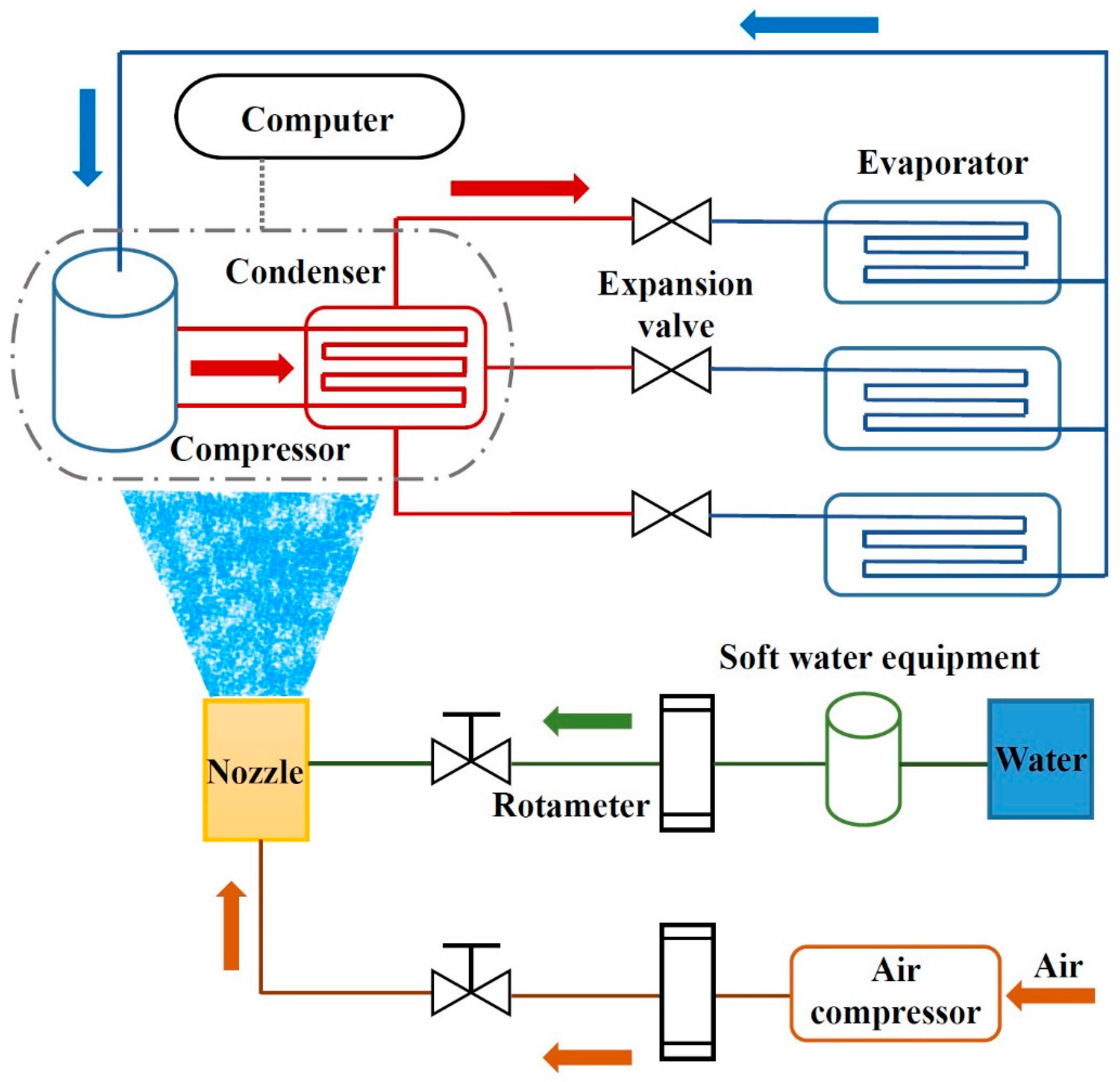
2.1. The Spray Cooling System

The spray cooling system has been an essential accessory in refrigeration systems. Specifically, it reduces the air inlet temperature by evaporating water into the humid air to precool the air to close to its wet-bulb temperature. As a result, the condensing temperature decreases, reducing the compressor unit’s energy consumption. However, the optimized set-up for evaporative cooling has yet to be clarified and needs an in-depth study. Figure 1 shows the spray cooling schematic for a standard evaporative cooling system. It can be seen that the system requires a nozzle used to atomise the water into smaller droplets. The droplet sizes would be as small as possible for a better evaporating effect, but this would consume much pressure from the pump, ultimately consuming power. The nozzle is the primary part of the spray cooling system. Whether the water droplets could have better heat and mass transfer depends on the atomisation quality. For the below case, the authors used a nozzle that could be adjusted voluntarily to meet different requirements. A standard spray cooling system mainly includes the spray system, heat exchanger, and measurement instruments. For the spray system, the main components should be spray nozzle, check valve, air compressor, pressure control valve, pressure gauge, water pipes, and shut-off valve. Commonly, tap water would be the primary source used for the spray system.

Figure 2 demonstrates a wind tunnel experiment where the water drops from a hollow-cone sheet. There are two thermocouples located upstream to measure the inlet and outlet water temperature. A pressure gauge was also used to measure water pressure. Wind tunnel experiments with an investigation of a hollow-cone nozzle spray performance were firstly conducted by Sureshkumar et al. [21] and Montazeri et al. [25]. The authors used a special technique to analyse the images for the droplet diameter distribution.

2.2. Spray and Turbulent Models

The Eulerian–Lagrangian method is applied to solve the problem in this study. Equations are used for tracking the position of droplets, velocity, energy, and mass as follows:

$$\frac{d{\overrightarrow{X}}_p}{dt}={\overrightarrow{V}}_p$$

(1)

The momentum balance is used only for drag and gravity effects as Equation (2). Other forces are not involved due to their insignificant effect on cases similar to this study [24].

$$m_p\frac{d{\overrightarrow{X}}_p}{dt}=C_D{\rho }_f\frac{\pi d_p^2}{8}{V}_r^2\frac{{\overrightarrow{V}}_r}{‖{\overrightarrow{V}}_r‖}+\frac{\pi d_p^3}{6}\left({\rho }_p-{\rho }_f\right)\overrightarrow{g}$$

(2)

The energy balance is applied for convection and evaporation effects based on the evaporation model from Abramzon and Sirignano [29] as follows:

$${\rho }_p\frac{\pi d_p^3}{6}{Cp}_p\frac{d{T}_p}{dt}={\dot{m}}_{vapor}\left[\frac{{Cp}_v\left(T_f-T_s\right)}{B_T}-L_v\right]$$

(3)

$$\frac{d{d}_p^3}{dt}=-\frac{6}{{\rho }_p\pi }{\dot{m}}_{vapor}$$

(4)

This study considers the tracking for a simple deposition of the droplet when contacting the wall. The evaporation rate is expressed as follows:

$${\dot{m}}_{vapor}=\pi d_p{Nu}^{*}\frac{{\lambda }_m}{C{p}_m}\ln \left(1+B_T\right)$$

(5)

$${Nu}^{*}=2+\frac{N{u}_0-2}{F_T}\mathrm{by}{F}_T={\left(1+B_T\right)}^{0.7}\frac{\ln \left(1+B_T\right)}{B_T}\mathrm{and}N{u}_0=1+{\left(1+{Re}_p{Pr}_m\right)}^{1/3}g\left({Re}_p\right)\mathrm{with}g\left({Re}_p\right)=max\left(1,{Re}_p^{0.077}\right)$$

(6)

where ${Nu}^{*}$ is the modified Nusselt number, which is used to model the convective exchange around the droplet. By this, ${Nu}^{*}$ is used as a function of the basic Nusselt number for a sphere in a given flow as $N{u}_0$ and a function $F_T$ of the so-called Spalding number for heat transfer as $B_T$. ${Re}_p$ is the particle Reynolds number, which is denoted ${Re}_p=\frac{{\rho }_f{d}_p‖{\overrightarrow{U}}_f-{\overrightarrow{V}}_p‖}{{\mu }_f}$, while $‖{\overrightarrow{U}}_f-{\overrightarrow{V}}_p‖$ is the relative velocity between fluid and dispersed phases. In terms of $B_T$, it can be obtained with the equivalent Spalding number for mass transfer $B_M$ in the following relations:

$$\left(1+B_T\right)={\left(1+B_M\right)}^{\frac{{Sh}^{*}}{{Nu}^{*}}\frac{1}{{Le}_m}}\mathrm{and}{B}_M=\frac{Y_{sat}-Y_f}{1-Y_{sat}}$$

(7)

where ${Le}_m$ is the Lewis number and ${Sh}^{*}$ is the modified Sherwood number, which can be expressed as follows:

$${Le}_m=\frac{{\lambda }_m}{{Cp}_m{\rho }_{m}D}$$

(8)

$$F_M=\frac{{Sh}_0-2}{{Sh}^{*}-2}\mathrm{with}{F}_M={\left(1+B_M\right)}^{0.7}\frac{\ln \left(1+B_M\right)}{B_M}\mathrm{and}{Sh}_0=1+{\left(1+{Re}_p{Pr}_m\right)}^{1/3}g\left({Re}_p\right)\mathrm{with}g\left({Re}_p\right)=max\left(1,{Re}_p^{0.077}\right)\mathrm{and}Sc=\frac{{\mu }_m}{D{\rho }_m}$$

(9)

For the calculation of $B_T$, an iterative process is applied in order to obtain the convergence value due to the relationship between ${Nu}^{*}$ and $B_T$ from Equations (6)–(9). Based on Tissot et al. [24], the new mass of the droplet can be calculated with the new diameter of itself based on the cubic root of the droplet’s volume from Equation (4). A specific drag coefficient is employed for drag modification due to evaporation phenomena [30].

$$C_D=\frac{24}{{Re}_p}\left(1+\frac{{Re}_p^{2/3}}{6}\right)$$

(10)

Under air inlet velocity (1 m/s) and wind tunnel geometry (380 × 260 mm), the Reynolds number for this condition is around 22,056. Therefore, the turbulent condition is applied under the realizable k-ε turbulence model for the present study. This model is selected as it provides more accuracy and less computational time [31,32]. The governing equations of the heat transfer and turbulent flow for the fluid can be seen in the following equations [31,32].

Continuity:

$$\frac{\mathsf{\partial }{U}_i}{\mathsf{\partial }{x}_i}=0$$

(11)

Momentum:

$$\rho U_i\frac{\mathsf{\partial }{U}_i}{\mathsf{\partial }{x}_i}=-\frac{\mathsf{\partial }P}{\mathsf{\partial }{x}_j}+\frac{\mathsf{\partial }}{\mathsf{\partial }{x}_i}\left[\mu \left(\frac{\mathsf{\partial }{U}_i}{\mathsf{\partial }{x}_j}+\frac{\mathsf{\partial }{U}_j}{\mathsf{\partial }{x}_i}\right)-\overline{\rho u_i^{\prime }{u}_j^{\prime }}\right]$$

(12)

Energy:

$$\rho C_p{U}_i\frac{\mathsf{\partial }T}{\mathsf{\partial }{x}_i}=\frac{\mathsf{\partial }}{\mathsf{\partial }{x}_i}\left[\lambda \frac{\mathsf{\partial }T}{\mathsf{\partial }{x}_j}-\rho C_p\overline{u_i^{\prime }{T}^{\prime }}\right]$$

(13)

where $U_i$ and T are the time-averaged velocity and temperature. The average Reynolds stresses and turbulent heat fluxes are defined as $\overline{\rho u_i^{\prime }{u}_j^{\prime }}$ and $\rho C_p\overline{u_i^{\prime }{T}^{\prime }}$, respectively.

The kinetic energy equation is expressed as:

$$\frac{\mathsf{\partial }}{\mathsf{\partial }t}\left(\rho k_t\right)+\frac{\mathsf{\partial }}{\mathsf{\partial }{x}_j}\left(\rho k_t{u}_j\right)=\frac{\mathsf{\partial }}{\mathsf{\partial }{x}_j}\left[\left(\mu +\frac{{\mu }_t}{{\sigma }_{k_t}}\right)\frac{{\mathsf{\partial }k}_t}{\mathsf{\partial }{x}_j}\right]+G_{k_t}+G_b-\rho {\epsilon }_t-Y_M+S_{k_t}$$

(14)

The dissipation rate of the turbulent kinetic energy equation is defined as:

$$\frac{\mathsf{\partial }}{\mathsf{\partial }t}\left(\rho {\epsilon }_t\right)+\frac{\mathsf{\partial }}{\mathsf{\partial }{x}_j}\left(\rho {\epsilon }_t{u}_j\right)=\frac{\mathsf{\partial }}{\mathsf{\partial }{x}_j}\left[\left(\mu +\frac{{\mu }_t}{{\sigma }_{{\epsilon }_t}}\right)\frac{{\mathsf{\partial }\epsilon }_t}{\mathsf{\partial }{x}_j}\right]+\rho C_{1}S{\epsilon }_t-\rho C_2\frac{{\epsilon }_t^2}{k_t+\sqrt{v{\epsilon }_t}}+C_{1,{\epsilon }_t}\frac{{\epsilon }_t}{k_t}{C}_{3,{\epsilon }_t}{G}_b+S_{{\epsilon }_t}$$

(15)

where the constant coefficients can be defined as $C_1=1.47$, $C_2=1.92$, ${\sigma }_{k_t}=1.0$, and ${\sigma }_{{\epsilon }_t}=1.3$. The turbulence kinetic energy productions induced by mean velocity gradients and buoyancy are $G_{k_t}$ and $G_b$, respectively. $Y_M$ is the contribution of the fluctuating dilatation in the incompressible turbulence to the overall dissipation rate. The turbulent viscosity is defined as ${\mu }_t=\rho C_{\mu }\frac{{k_t}^2}{{\epsilon }_t}$. The turbulent intensity is calculated based on the average Reynolds number at inlets by $I=0.16{\left({Re}_{D_h}\right)}^{-0.125}$.

2.3. Boundary Conditions and Operating Parameters

In terms of the boundary conditions, the numerical inputs for the simulation are as follows: the air is used as the primary phase, which is injected from the inlet of wind tunnel at a temperature of 298 K and average velocity of 1 m/s. The relative humidity is set at 30% of relative humidity. For the secondary phase, the water is used as the droplet with size ranges from 25 µm to 50 µm (as a uniform method) for validation with the case study of Tissot et al. [24]. The droplets would be injected with an angle of 72 degrees and in a cone shape. The temperature of the injected droplets is set at 298 K, and the velocity is 10 m/s. The spray pressure is fixed for all droplets. The same initial velocities for air inlet and droplet from the study by Tissot et al. [24] are applied to simulate all cases in the present study. At the outlet, the zero-gauge pressure condition is selected for all cases.

To analyse the spray cooling performance over Australian regions, the Rosin–Rammler method is used with droplet size of 25 µm to 100 µm. However, the humidity and temperature of the air are varied due to the different weather conditions in different regions in Australia. For humidity, the species mass fractions are used as the humidity input data, which are obtained from the humidity ratio (kg_vapour/kg_{dry air}) from the psychrometric chart [33]. The input parameters to obtain the humidity ratio (x) are the dry-bulb temperature and relative humidity. These two parameters can be taken from the measurement in each Australia’s region, which can be seen under the numerical method and settings in 3.3 Australian ambient conditions section.

In terms of spray nozzle characteristics, ANSYS Fluent provides an option of a hollow cone spray model to simulate the spray effect. In this study, the spray nozzle was set as a cone spray with an injection angle of 72 degrees. Specifically, a pointed nozzle was specified to inject droplets into the computational domain. The location of the nozzle was set at X = 0.42 m, Y = 0, Z = 0. The total mass flow rate and temperature were set as boundary conditions. A total of 110,400 particles were set to be an injection for the spray cooling for model validation under the uniform method with 25 µm to 50 µm. Figure 3 shows the wind tunnel with the spray nozzle and injected water for the co-flow direction. In this case, the direction of the spray nozzle is set as the same direction of the airflow. Figure 4 shows the wind tunnel with the spray nozzle and injected water for counter-flow direction. In counter-flow, the spray nozzle is set in the opposite direction to the airflow at the inlet of the wind tunnel.

Using ANSYS Fluent, the coupled scheme is selected for the pressure–velocity coupling. The second-order method is selected for pressure variables. The second-order upwind scheme is applied for the momentum and other parameters. For the relaxation factors, 0.5 is set for pressure and momentum, while 0.75 is set for energy and all velocity components. For discrete phase sources, the relaxation factor is set as 0.9. The convergence criteria are set as 10⁻⁴ for all parameters except energy, which has a convergence criterion of 10⁻⁶.

3. Numerical Method and Settings

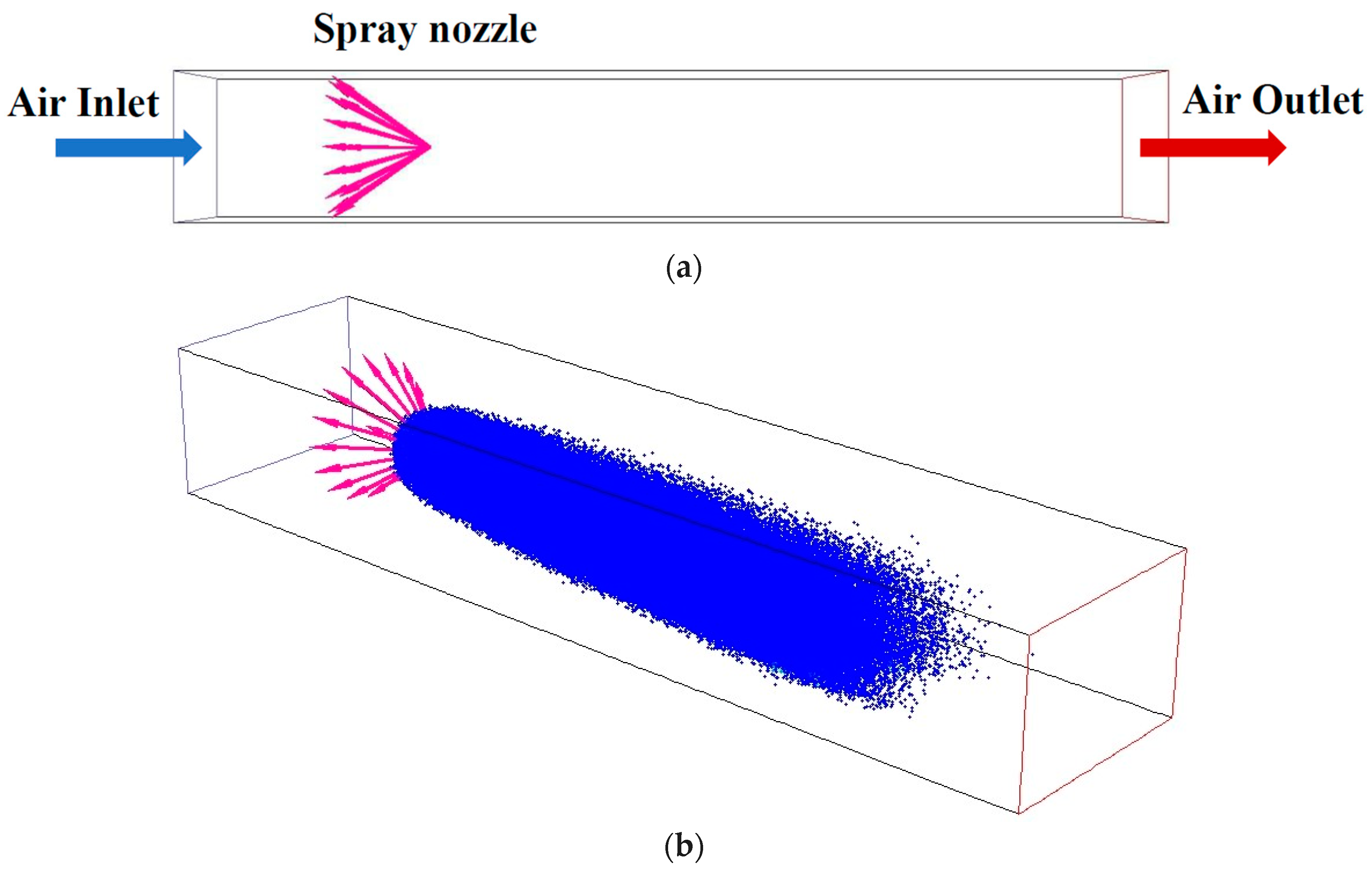
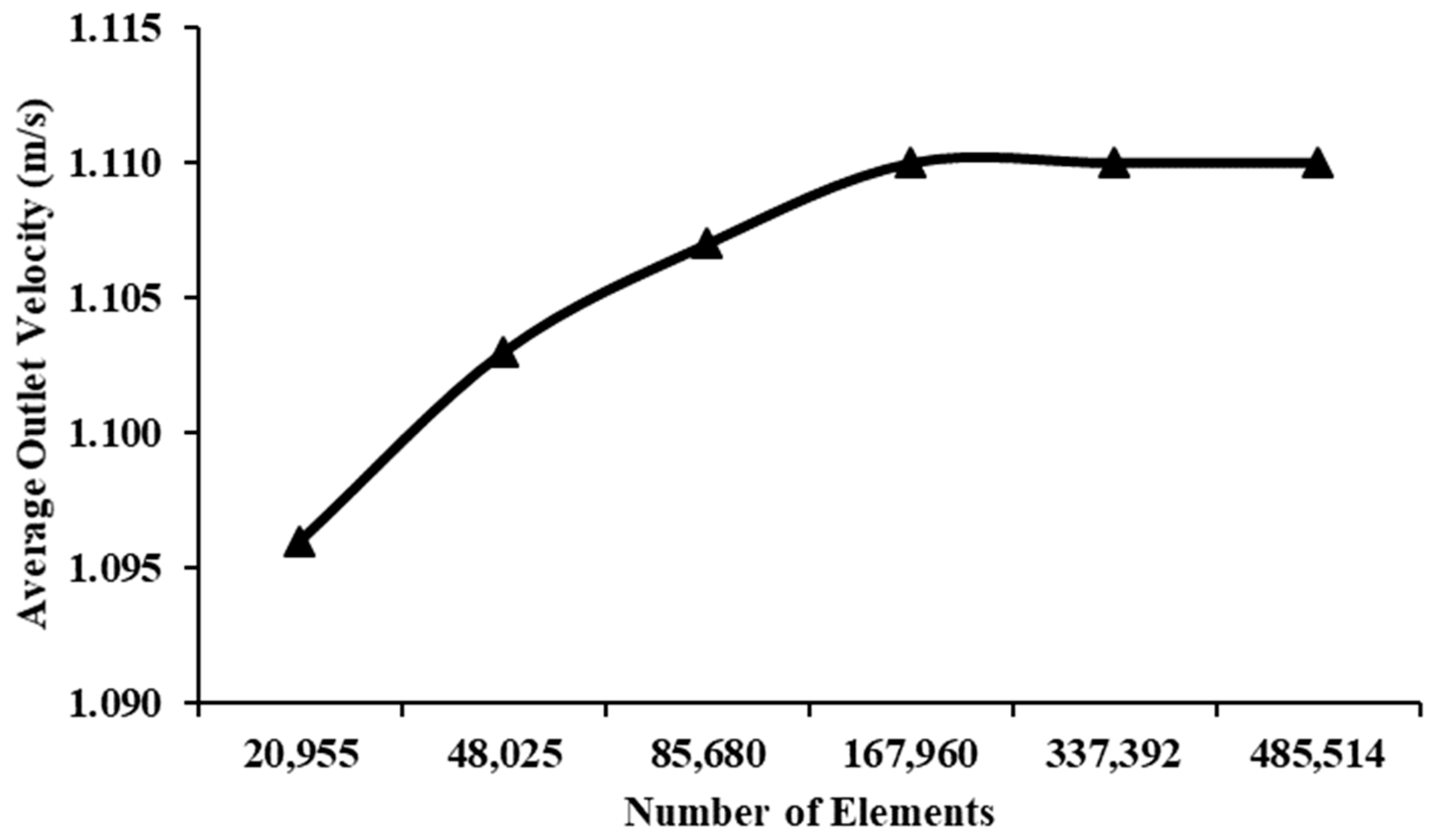
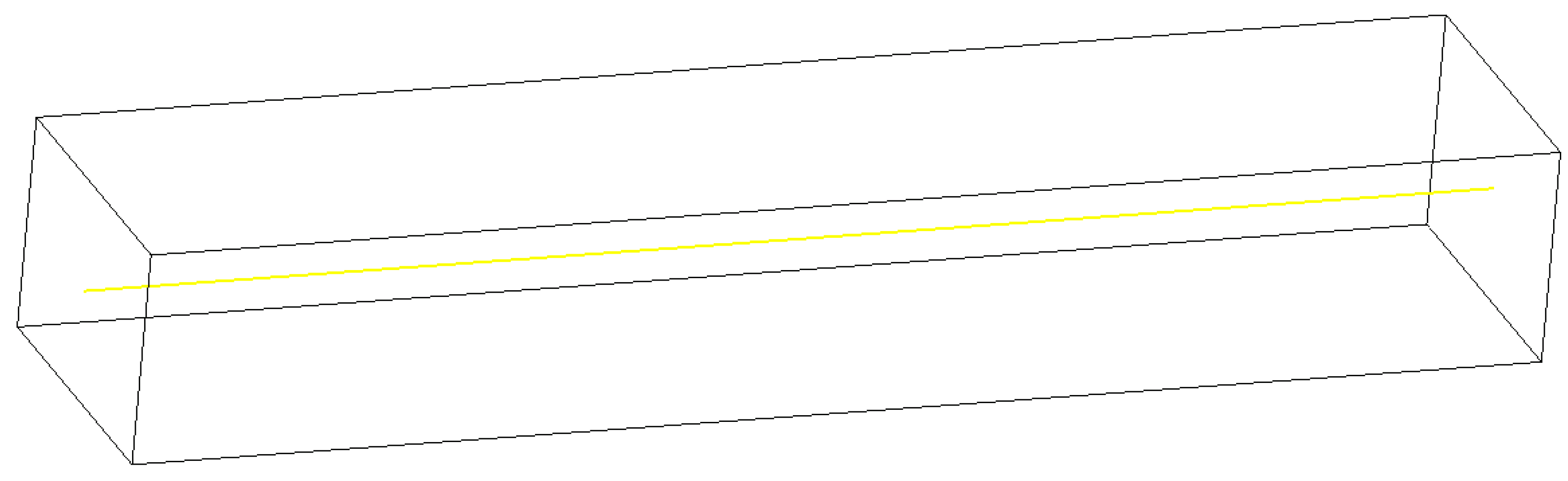
3.1. Computational Geometry and Grid Independence Test

Figure 5 shows the wind tunnel geometry. In this study, the wind tunnel was modelled based on the wind tunnel dimension from Tissot et al. [24] by Design Modeller, which is the software function of ANSYS. The tunnel length would be 1700 mm, while the cross-section is 380 × 260 mm. The ANSYS meshing module was employed to create a hexahedron mesh with an element size of 10 mm. Figure 6 illustrates the mesh for the whole geometry and two different planes. Inflation layers are used for the system, and 10 inflation layers are applied. The minimum orthogonal mesh quality is 0.71.

Figure 7 presents the grid refinement test. A grid refinement is performed until a specific result remains unchanged to verify whether the given mesh is reasonable to proceed with further analysis. In this case, the average outlet air velocity is examined by using seven different element quantities. In terms of the boundary conditions for the grid independence test, the velocity of the air inlet was set as 1 m/s.

From Figure 7, it can be seen that the average outlet velocity increases gradually from 1.096 m/s to 1.11 m/s. From the number elements of 167,960, the velocity remains constant at 1.11 m/s. It is clear that from this number, the simulated results would be independent of the element number.

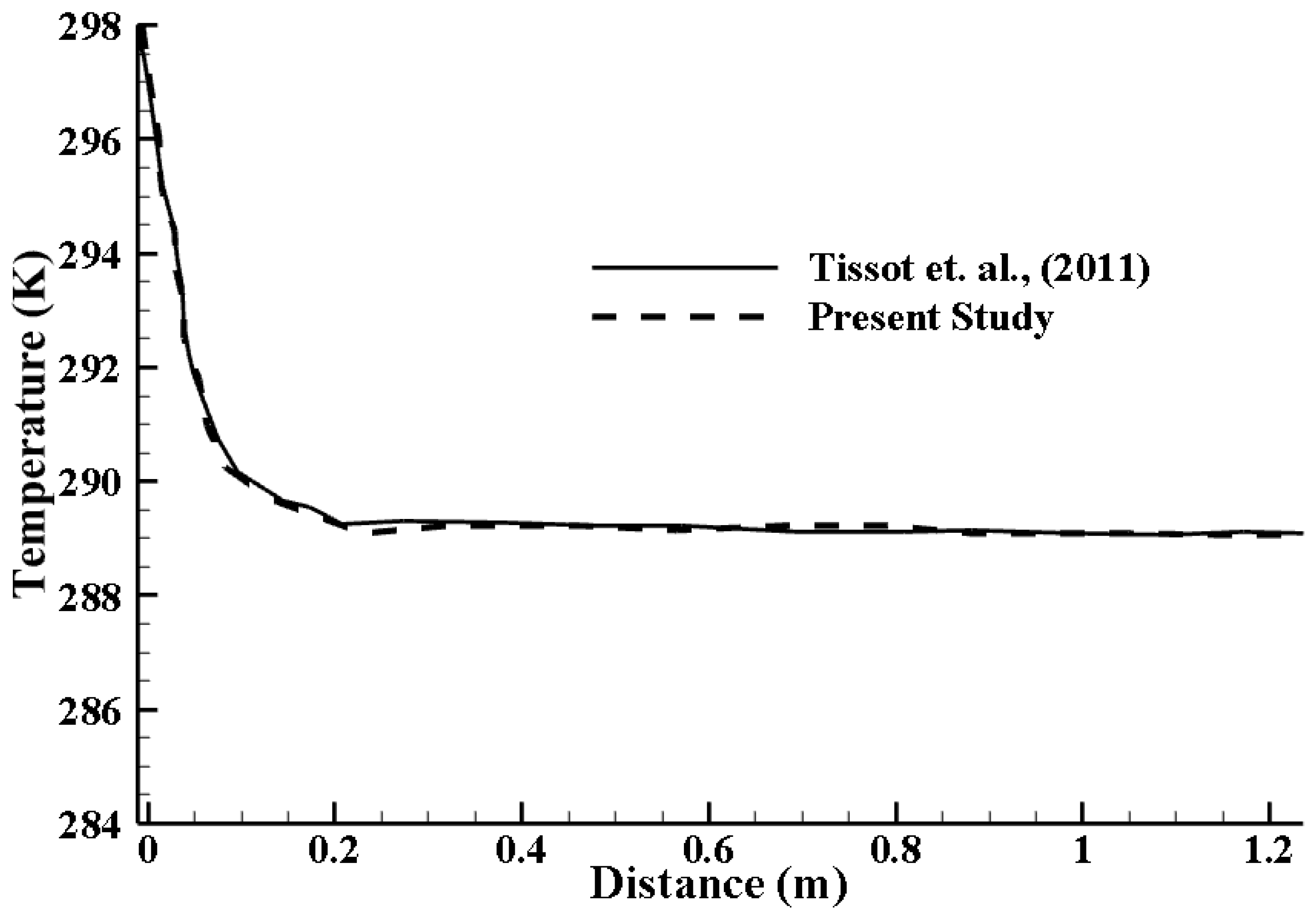
3.2. Model Validation

In the context of simulation, the validation process is conducted to ensure the accuracy of the final model. The users and decision-makers, who use the results obtained from the simulation, can arrive at the correct decision and analysis for specific engineering problems. Therefore, simulation validation is a crucial and fundamental step before proceeding with further analysis.

In the co-flow configuration, the air will be blown in the same direction as the injected droplets. The droplet sizes vary from 25 µm to 50 µm. The temperature contour at the midplane in the Y-axis (Y = 1.9 m) was created in order to compare to Tissot et al.’s [24] case. The model validation between the study from Tissot et al. [24] and the present study is presented in Figure 8 as the temperature contour. In this case, a conic spray of the 50 µm droplets was injected in a co-flow direction with the air. Additionally, the temperature along the spray is also depicted on the right-hand side. It can be seen that the water droplets travelled along with the airflow on the rectilinear path with a limited impact from turbulent dispersion. Furthermore, the droplets are more inclined downward due to the gravity effect. As predicted, the air temperature decreases by up to 10 °C due to the evaporating effect as the air temperature comes close to its wet-bulb temperature. From the temperature contour, there is an alignment between Tissot’s study and the present study. The temperature ranges from 288 K to 298 K for both cases. On the outer layer of the spray, the temperature is at its peak of 298 K as it has direct contact with the water vapour and the airflow. Additionally, the temperature decreases when it comes to the centre of the spray. It should be noted that the variation in temperature differences between these two studies might come from the different values of the temperature range. Although the minimum and maximum temperatures from these studies are the same, 288 K and 298 K, the temperature range from Tissoit’s study increases by 2 numbers for each step, while the temperature range from the present study increases by only 1 number for each step. Therefore, the mean temperature comparison between these studies is performed for accuracy purposes.

In the sprayed airflow, one of the most important parameters is the droplet size. In Figure 9, the temperature distribution along the axial position x = 1.42 m is presented by examining 1 m away from the nozzle. It can be seen there is a heterogeneous temperature of the air, which is impacted in the centre of the spray. The other important observation is the effect of droplet size, where the different diameters of 50 µm to 25 µm are dispersed. It shows that the smaller droplet size has a stronger influence on the ambient air. However, the spray could only cool the air in a small restricted area, while other surfaces remain the same. For larger droplets, it is less efficient for cooling the air. In general, the CFD analysis and Tissot et al. [24] are similar, so the model is accurate to perform co-flow simulation.

3.3. Australian Ambient Conditions

Spanning almost 7.7 million km², there is a range of different climate zones affecting Australia. According to Geoscience Australia [34], the temperature range in Australian regions varies from an average high temperature of 40 °C in the central desert regions to below freezing in the southeast of the country. The average annual rainfall is low over most of the continent, but it receives intense seasonal fall in the tropics. The wettest regions are Queensland and Tasmania. Based on the available data of the average mean temperature and humidity from the Australian Bureau of Meteorology 2021 [35], the mean temperature and relative humidity at 3 pm in six different major cities ae provided in

Table 1. Australian temperatures and humidity at 3 pm for major cities [35].

		Australian Temperature at 3 pm (°C)
Location	City	Jan	Feb	Mar	Apr	May	Jun	Jul	Aug	Sep	Oct	Nov	Dec
SA	Adelaide	25.9	26.3	23.9	20.8	17.5	15.0	14.0	14.8	16.7	19.2	21.9	23.6
QLD	Brisbane	28.8	28.2	27.1	25.0	22.8	20.5	20.2	21.4	23.6	25.1	26.4	27.8
NT	Darwin	30.2	30.0	30.5	31.7	31.2	29.9	29.6	30.2	31.2	32.0	31.9	31.2
VIC	Melbourne	24.3	24.8	22.5	19.0	15.6	12.6	12.0	13.2	15.2	17.6	20.2	22.4
WA	Perth	29.9	30.2	28.1	24.2	20.6	17.8	16.8	17.3	18.8	21.1	24.2	27.1
NSW	Sydney	24.8	24.8	23.9	21.7	19.0	16.6	16.1	17.2	19.0	20.7	22.1	23.9
		Australian Humidity at 3 pm (%)
Location	City	Jan	Feb	Mar	Apr	May	Jun	Jul	Aug	Sep	Oct	Nov	Dec
SA	Adelaide	42	42	46	50	58	64	65	61	56	50	46	45
QLD	Brisbane	55	58	56	54	53	51	45	43	45	50	53	54
NT	Darwin	70	72	67	52	43	38	37	40	47	52	58	65
VIC	Melbourne	44	44	47	52	60	67	65	59	56	52	49	45
WA	Perth	37	37	39	46	53	60	60	56	54	49	44	41
NSW	Sydney	60	63	61	59	58	57	52	49	51	54	56	58

. This available data are then used as the input data from the CFD simulations.

From Table 1, it can be seen that the temperature changes in a similar way for all the regions, where the highest temperature is in January and December, and the lowest temperature is between June and August. Moreover, Darwin stands out as the hottest city of the six regions. The humidity chart displays a different trend, whereby Perth, Adelaide, and Melbourne reach their peak in June at around 60% relative humidity. In contrast, the highest humidity in Darwin, Sydney, and Brisbane is in January and December.

4. Results and Discussion

4.1. The Effect of Spray Cooling

The simulation model is now utilized for six major cities in Australia: Adelaide, Brisbane, Darwin, Melbourne, Perth, Sydney. The ambient conditions for each city, including the temperature and humidity from Table 1, are set as the boundary conditions in terms of inlet temperature and inlet humidity. The simulations were separately conducted for each month in each city. Figure 10 shows the comparison between the input and output data from both temperature and humidity. Figure 10a,c presents the input data (based on the average mean temperature and humidity from the Bureau of Meteorology [35]) as the inlet temperature and inlet humidity. Figure 10b,d demonstrates the output data (located at the outlet of the wind tunnel) as the average outlet temperature and outlet humidity in different cities throughout the year.

From Figure 10a,b, it is clear that the outlet temperature is much lower than the inlet temperature in hot weather, such as in January and December. However, the temperature barely changes in winter conditions for Melbourne, Adelaide, and Perth in June. Sydney and Brisbane have a stable gap between outlet temperature and inlet temperature. Darwin has a different pattern from the other cities, where the temperature drops slightly in January and February and has a big difference from March to December. Melbourne, Adelaide, Sydney, Perth, Brisbane, and Darwin have a temperature from low to high throughout the year. Darwin is the most extreme city, which has an average temperature above 295 K (22 °C) in a year.

For the humidity (Figure 10c,d), the maximum achieved humidity remains stable above 90% relative humidity (the difference between inlet and outlet humidity); additionally, the relative humidity increases approximately 30% throughout the year for all the cities. Moreover, Darwin significantly changes in June and July from just under 40% relative humidity to just under 90%. This can be explained by the high temperature in Darwin during this period. Furthermore, the humidity at the inlet and outlet has the same patterns for each city. The maximum relative humidity is stable from May to September (Figure 10d), maximum relative humidity is stable from May to September (Figure 10d), while there is no stable level for inlet relative humidity (Figure 10c).

4.2. Psychometric Chart

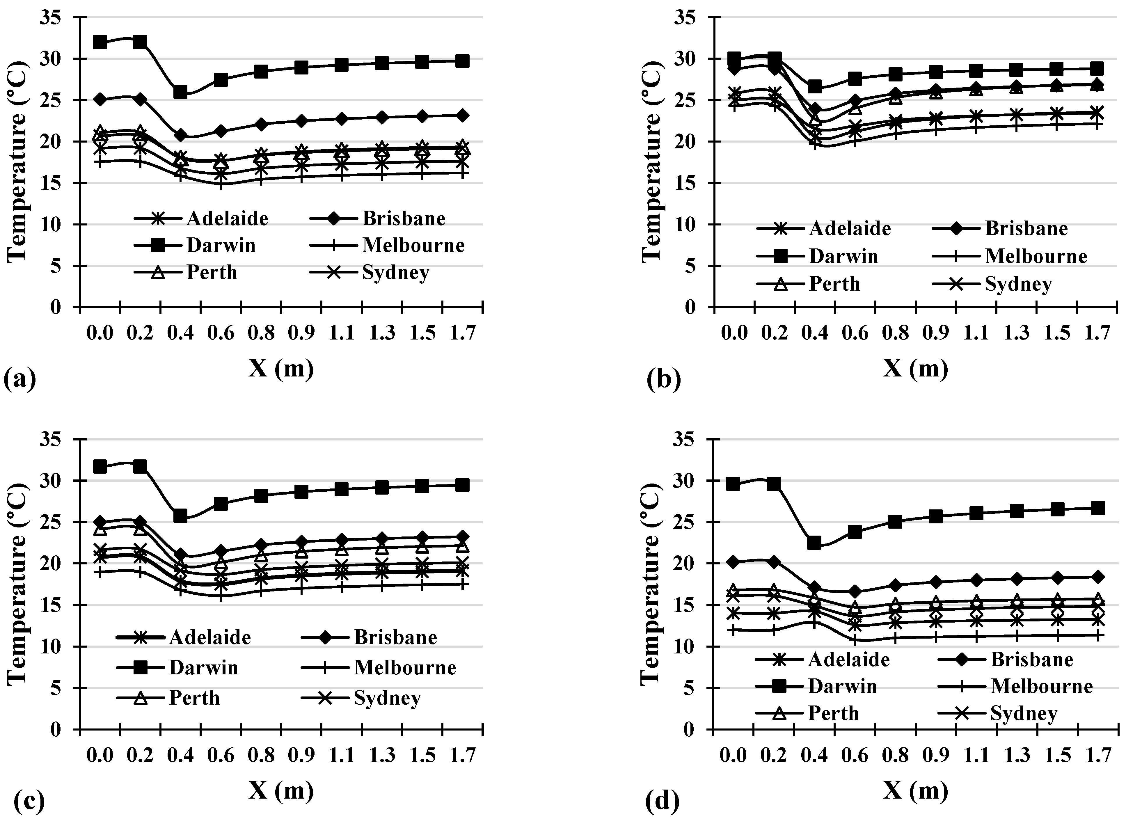
The psychometric chart is a useful tool to examine the relationship between ambient air temperature and moisture content. This chart gives the engineer the ability to look up the relevant parameters from the given air conditions. Figure 11 shows the evaporating effect on the psychometric chart for the six chosen cities in January. It is clear from the chart that Perth has the highest impact due to the spray cooling effect, where the temperature drops from 30 °C to 23 °C. Darwin has the least effect from the spray cooling, where the temperature only reduces by 4 °C. Adelaide is the second-most effective city wherein the temperature can be reduced by up to 7 °C. Melbourne, Sydney, and Brisbane showed equal improvement, with temperature reductions of 5 °C.

4.3. Profiles

In this analysis, a central line along the wind tunnel is given in Figure 12. Figure 13 presents the temperature profile for all six cities based on four seasons in a year. Figure 13a,b is the temperature profile for spring and summer, while Figure 13c,d is the temperature profile for autumn and winter. The temperature profile illustrates how the temperature of specific fluid changes by the specified coordinate.

In Figure 13, it can be seen that the temperature drops for all seasons and cities when the air contacts water, which evaporates and reaches its minimum at x = 0.38 m. After that, the temperature gradually increases due to the heat transfer between the air and the spray region. At the spray injection area, summer (Figure 13b) shows significant temperature drops for all cities, especially Perth, followed by Adelaide if compared to other seasons. Darwin has the highest temperature, while Melbourne has the lowest temperature for all seasons.

Figure 14 shows various profile parameters in January along the wind tunnel. Based on Figure 14a,c, the humidity and mass fraction patterns are the same for all the cities. Humidity and mass fraction increase dramatically when the water vapour is sprayed into the blowing air. In addition, Darwin has the highest mass faction if compared to other cities (Figure 14b). In terms of velocity and pressure profiles (Figure 14b,d), all cities have the same pressure and velocity magnitudes in total. The highest pressure, 0.35 Pa, is found at the contact area between the air and water vapours. In contrast, this contact area significantly generates the lowest-velocity magnitude—0.47 m/s.

4.4. Contours

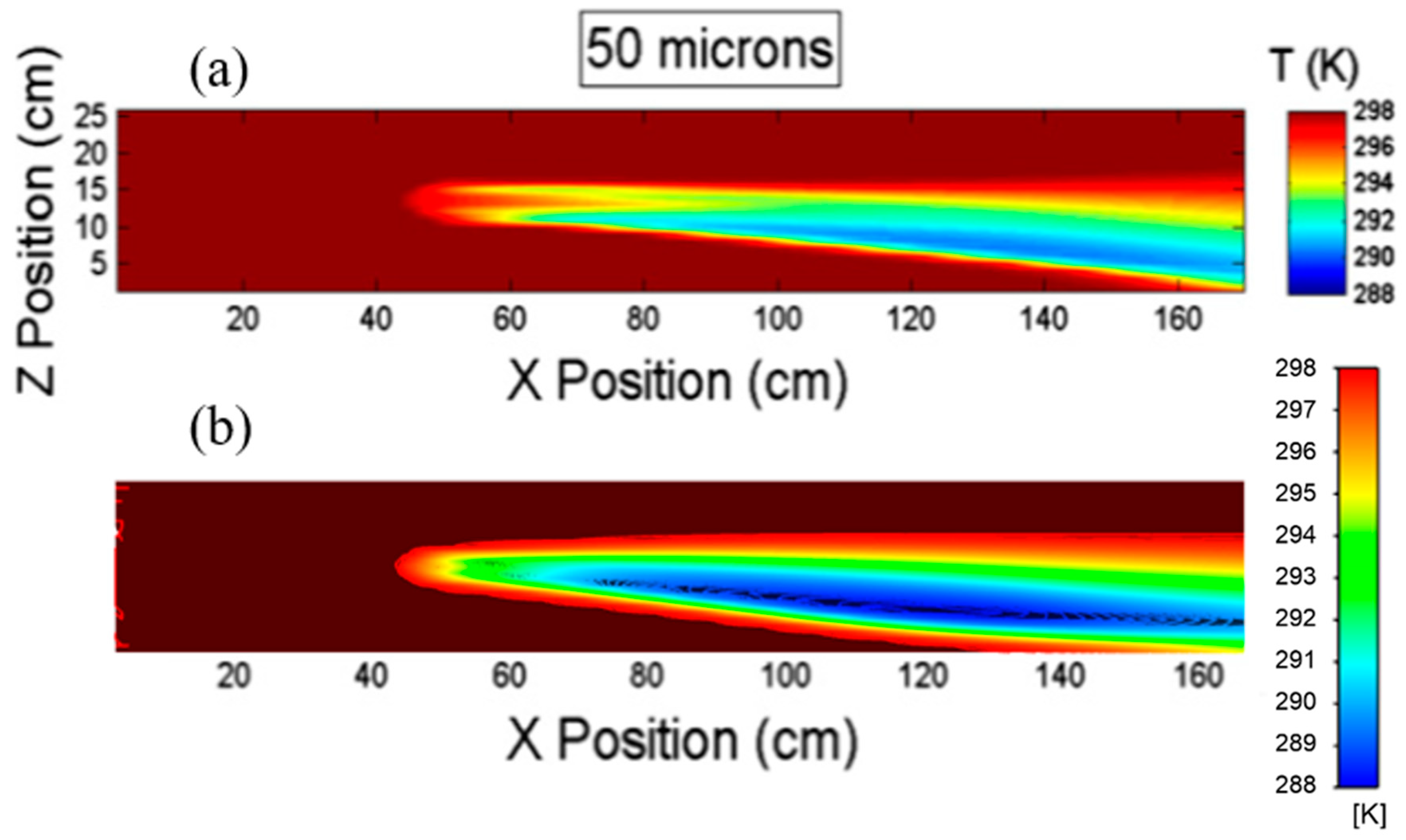
4.4.1. Temperature Contour

Figure 15 presents the temperature contours for all cities in January. Based on these contours, the minimum temperature locates at the centre of the contact area between the air and water vapour for all cities (injection area of spray nozzle). The maximum temperature locates at the initial area for all cities. Moreover, close to the edge of the top and bottom contours for all cities still have higher temperatures, which are very similar to the initial area. However, if the temperature range is considered, Darwin (Figure 15c) has the highest temperature, around 300 K to 303 K (27 $℃$ to 30 $℃$), following by Perth (Figure 15e) and Brisbane (Figure 15b). In comparison, other cities have a lower temperature, which is between 292 K and 300 K (19 $℃$ to 27 $℃$).

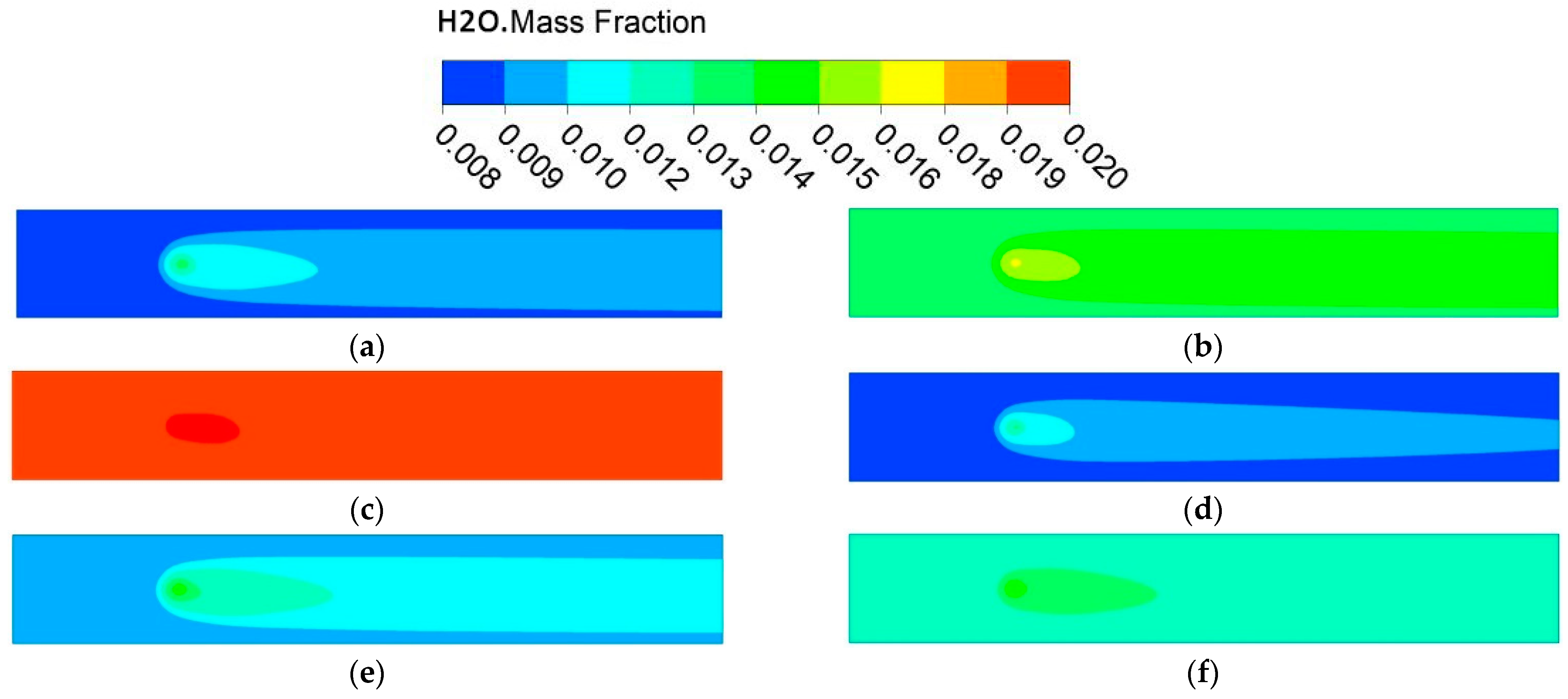
4.4.2. Mass Fraction Contour

Figure 16 presents the mass fraction contours for all cities in January. The maximum mass fraction is found at the spray injection area for all cities. The minimum mass fraction is found at the edges of the top and bottom areas for all cities. All cities have similar patterns for mass faction, except Darwin (Figure 16c), with a larger area regarding higher mass fraction magnitude. In terms of mass fraction ranges, Darwin has the highest mass fraction, 0.20, while Adelaide (Figure 16a) and Melbourne (Figure 16d) have the lowest mass fractions, around 0.008 to 0.015.

4.4.3. Pressure Contour

Pressure drops play a significant role in the required fan power. Figure 17 shows the pressure contours for all cities in January. All cities have similar pressure patterns. Due to the similar pressure patterns, there is only one pressure contour that is presented in this study. The maximum pressure of 0.387 Pa is found around the centre of the spray injection point. The initial area has a higher pressure, while a lower pressure occurs around the exit area. From this figure, it is evident that the pressure significantly drops from the inlet throughout the outlet of the wind tunnel. Based on Australia’s seasons, the average pressure at the inlet of the wind tunnel is 0.18 Pa. At the spray injection point, the average pressure is 0.09 Pa. At the outlet of the wind tunnel, the average pressure is 0.0002 Pa. These average pressures are for all seasons and all cities.

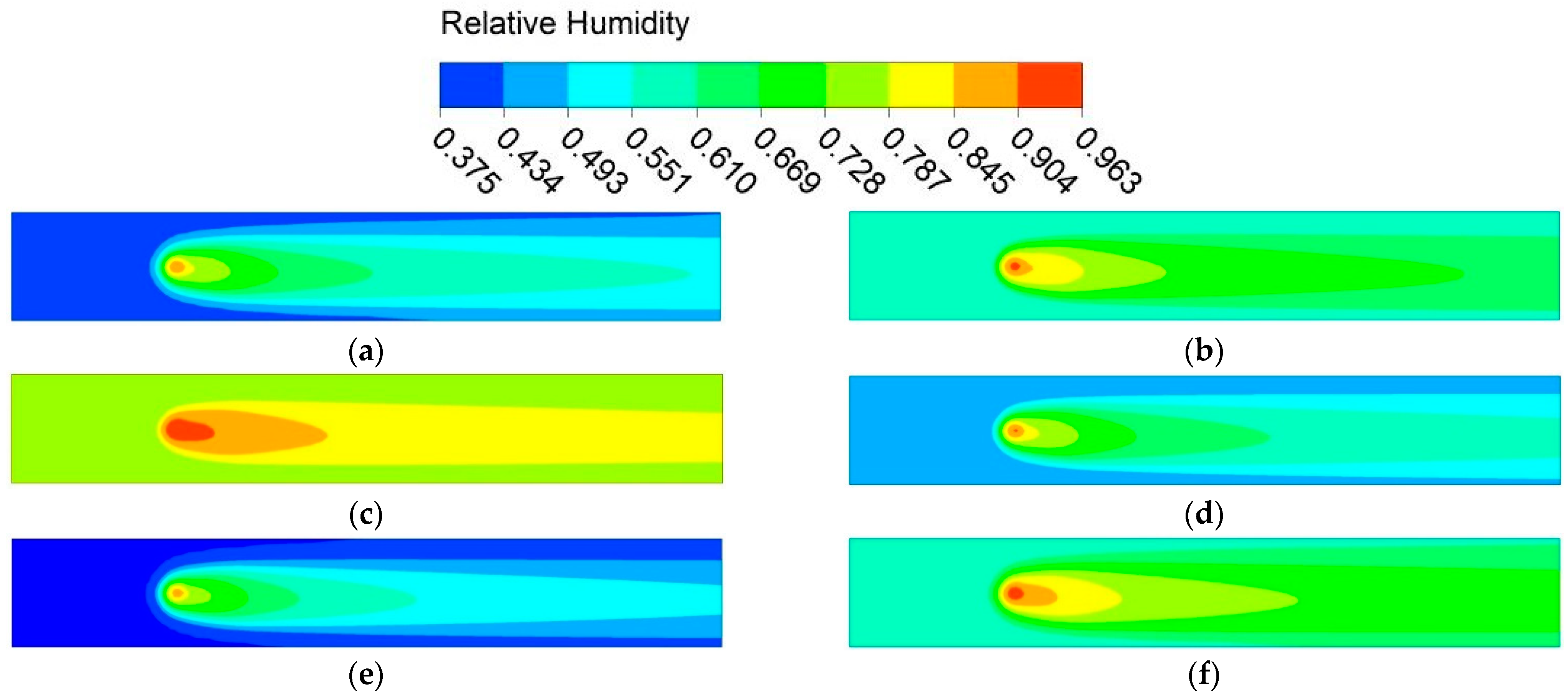
4.4.4. Relative Humidity Contour

The relative humidity contours in January were created and are presented in Figure 18. The maximum relative humidity of 0.963 is found at the centre of the spray injection point for all six cities. After that, it continually decreases throughout the exit. The minimum relative humidity is found at the initial area and nearly the edge of the top and bottom areas. If the relative humidity ranges are considered, Darwin (Figure 18c) has the highest relative humidity, followed by Sydney (Figure 18f) and Brisbane (Figure 18b). The lowest relative humidity, 0.375, is found in Perth (Figure 18e), followed by Adelaide (Figure 18a).

4.4.5. Velocity Contour

Figure 19 presents the velocity contour for all six cities in January. The velocity patterns and magnitude are the same for all six cities. Due to similar velocity patterns, there is only one velocity contour that is presented in this study. The maximum and minimum velocities are found around the spray injection area for all cases. Furthermore, areas close to the edge of the top and bottom have higher velocity magnitudes if compared to other areas.

5. Conclusions

In this study the spray cooling pattern, temperature, and humidity distribution, as well as the evaporation effect, have been investigated for six different regions in Australia, simulated based on the CFD technique. In terms of model validation, the results show strong agreement with the previous study by Tissot et al. [24]. For the application of spray cooling under different conditions in Australian regions, water droplet sizes ranging from 25 µm to 100 µm and the average ambient conditions were used as the input data for six cities throughout the year. The key findings are as follows:

-

It is clear that effective enhancement of cooling is achievable, as demonstrated by the temperature at the outlet being lower than the temperature at the inlet for all cities in hot weather, especially in summer, and particularly for Perth and Adelaide. In cold weather, especially in winter, the temperature barely changes for all cities, but it mainly affects three cities: Melbourne, Adelaide, and Perth.

-

For humidity, spray cooling influences the relative humidity pattern, especially the area close to spray injection. The relative humidity generally increases by approximately 30% (absolute) throughout the year for all cities. However, because of its high winter temperature, the relative humidity significantly changes in Darwin in winter, from just under 40% to almost 90%.

-

The pressure and velocity demonstrate the same patterns for all cities. The pressure is higher at the spray injection area. The flow and pressure are independent of season and location, because of air’s thermophysical properties, which are identical, and having only a one-way coupling between the fluid and particles. In other words, there is no dependence on temperature and the particles have no influence on the fluid flow.

For further studies, a spray with a combination of various droplet sizes will be considered to examine the real-life effect over different ambient conditions. The effect of droplet sizes will be further analysed in each Australian region, where there are different ambient conditions. Furthermore, the reactions between multiple nozzles will also be considered to compare the spray cooling system performance.

References

1. Zhang, Z.; Li, J.; Jiang, P.-X. Experimental investigation of spray cooling on flat and enhanced surfaces. Appl. Therm. Eng. 2013, 51, 102–111. [Google Scholar] [CrossRef]
2. Cheng, W.-L.; Zhang, W.-W.; Shao, S.-D.; Jiang, L.-J.; Hong, D.-L. Effects of inclination angle on plug-chip spray cooling in integrated enclosure. Appl. Therm. Eng. 2015, 91, 202–209. [Google Scholar] [CrossRef]
3. Sajjad, U.; Abbas, M.; Hamid, K.; Abbas, S.; Hussain, I.; Ammar, S.M.; Sultan, M.; Ali, H.M.; Hussain, M.; Rehman, T.; et al. A review of recent advances in indirect evaporative cooling technology. Int. Commun. Heat Mass Transf. 2021, 122, 105140. [Google Scholar] [CrossRef]
4. Costelloe, B.; Finn, D. Indirect evaporative cooling potential in air–water systems in temperate climates. Energy Build. 2003, 35, 573–591. [Google Scholar] [CrossRef] [Green Version]
5. Kim, J. Spray cooling heat transfer: The state of the art. Int. J. Heat Fluid Flow 2007, 28, 753–767. [Google Scholar] [CrossRef]
6. Tissot, J.; Boulet, P.; Trinquet, F.; Fournaison, L.; Lejeune, M.; Liaudet, F. Improved energy performance of a refrigerating machine using water spray upstream of the condenser. Int. J. Refrig. 2014, 38, 93–105. [Google Scholar] [CrossRef]
7. Jones, S.D.M.; Robertson, W.M. The effects of spray-chilling carcasses on the shrinkage and quality of beef. Meat Sci. 1988, 24, 177–188. [Google Scholar] [CrossRef] [PubMed]
8. Hynry, F.; Bennett, A. Hydraircooling vegetable products in unit loads. Trans. ASAE 1973, 16, 731–733. [Google Scholar] [CrossRef]
9. Létang, G.; Moureh, J. Application de la brumisation dans les meubles de vente pour denrées alimentaires fraîches. Rev. Gén. Froid. 2005, 1057, 51–66. [Google Scholar]
10. Naticchia, B.; D’Orazio, M.; Carbonari, A.; Persico, I. Energy performance evaluation of a novel evaporative cooling technique. Energy Build. 2010, 42, 1926–1938. [Google Scholar] [CrossRef]
11. Pearlmutter, D.; Erell, E.; Etzion, Y.; Meir, I.; Di, H. Refining the use of evaporation in an experimental down-draft cool tower. Energy Build. 1996, 23, 191–197. [Google Scholar] [CrossRef]
12. Wang, J.-X.; Li, Y.-Z.; Yu, X.-K.; Li, G.-C.; Ji, X.-Y. Investigation of heat transfer mechanism of low environmental pressure large-space spray cooling for near-space flight systems. Int. J. Heat Mass Transf. 2018, 119, 496–507. [Google Scholar] [CrossRef]
13. Hou, Y.; Tao, Y.; Huai, X.; Guo, Z. Numerical characterization of multi-zone spray cooling. Appl. Therm. Eng. 2012, 39, 163–170. [Google Scholar] [CrossRef]
14. Al-Waked, R.; Behnia, M. CFD simulation of wet cooling towers. Appl. Therm. Eng. 2006, 26, 382–395. [Google Scholar] [CrossRef]
15. Kim, K.; Yoon, J.-Y.; Kwon, H.-J.; Han, J.-H.; Son, J.E.; Nam, S.-W.; Giacomelli, G.A.; Lee, I.-B. 3-D CFD analysis of relative humidity distribution in greenhouse with a fog cooling system and refrigerative dehumidifiers. Biosyst. Eng. 2008, 100, 245–255. [Google Scholar] [CrossRef]
16. Somasundaram, S.; Tay, A.A.O. A study of intermittent liquid nitrogen sprays. Appl. Therm. Eng. 2014, 69, 199–207. [Google Scholar] [CrossRef]
17. Liu, X.; Xue, R.; Ruan, Y.; Chen, L.; Zhang, X.; Hou, Y. Flow characteristics of liquid nitrogen through solid-cone pressure swirl nozzles. Appl. Therm. Eng. 2017, 110, 290–297. [Google Scholar] [CrossRef]
18. Liu, X.; Xue, R.; Ruan, Y.; Chen, L.; Zhang, X.; Hou, Y. Effects of injection pressure difference on droplet size distribution and spray cone angle in spray cooling of liquid nitrogen. Cryogenics 2017, 83, 57–63. [Google Scholar] [CrossRef]
19. Xue, R.; Ruan, Y.; Liu, X.; Chen, L.; Zhang, X.; Hou, Y.; Chen, S. Experimental study of liquid nitrogen spray characteristics in atmospheric environment. Appl. Therm. Eng. 2018, 142, 717–722. [Google Scholar] [CrossRef]
20. Montazeri, H.; Blocken, B.; Hensen, J.L.M. CFD analysis of the impact of physical parameters on evaporative cooling by a mist spray system. Appl. Therm. Eng. 2015, 75, 608–622. [Google Scholar] [CrossRef] [Green Version]
21. Sureshkumar, R.; Kale, S.R.; Dhar, P.L. Heat and mass transfer processes between a water spray and ambient air—I. Experimental data. Appl. Therm. Eng. 2008, 28, 349–360. [Google Scholar] [CrossRef]
22. Zhang, W.; Cheng, W.; Shao, S.; Jiang, L.; Hong, D. Integrated thermal control and system assessment in plug-chip spray cooling enclosure. Appl. Therm. Eng. 2016, 108, 104–114. [Google Scholar] [CrossRef]
23. Ho Song, C.; Lee, D.; Tack Ro, S. Cooling enhancement in an air-cooled finned heat exchanger by thin water film evaporation. Int. J. Heat Mass Transf. 2003, 46, 1241–1249. [Google Scholar] [CrossRef]
24. Tissot, J.; Boulet, P.; Trinquet, F.; Fournaison, L.; Macchi-Tejeda, H. Air cooling by evaporating droplets in the upward flow of a condenser. Int. J. Therm. Sci. 2011, 50, 2122–2131. [Google Scholar] [CrossRef]
25. Montazeri, H.; Blocken, B.; Hensen, J. Evaporative cooling by water spray systems: CFD simulation, experimental validation and sensitivity analysis. Build. Environ. 2015, 83, 129–141. [Google Scholar] [CrossRef]
26. Xia, L.; Gurgenci, H.; Liu, D.; Guan, Z.; Zhou, L.; Wang, P. CFD analysis of pre-cooling water spray system in natural draft dry cooling towers. Appl. Therm. Eng. 2016, 105, 1051–1060. [Google Scholar] [CrossRef] [Green Version]
27. Kabeel, A.D.; EI-Samadony, Y.A.F.; Khiera, M.H. Performance evaluation of energy efficient evaporatively air-cooled chiller. Appl. Therm. Eng. 2017, 122, 204–213. [Google Scholar] [CrossRef]
28. Yang, H.; Rong, L.; Liu, X.; Liu, L.; Fan, M.; Pei, N. Experimental research on spray evaporative cooling system applied to air-cooled chiller condenser. Energy Rep. 2020, 6, 906–913. [Google Scholar] [CrossRef]
29. Abramzon, B.; Sirignano, W.A. Droplet vaporisation model for spray combustion calculations. Int. J. Heat Mass Transf. 1989, 32, 1605–1618. [Google Scholar] [CrossRef]
30. Faeth, G.M. Current status of droplet and liquid combustion. Prog. Energy Combust. Sci. 1977, 3, 499–539. [Google Scholar] [CrossRef]
31. Xiong, M.; Chen, B.; Zhang, H.; Qian, Y. Study on accuracy of CFD simulation of wind environment around high-rise building: A comparative study of k-ε turbulence models based on polyhedral meshes and wind tunnel experiments. Appl. Sci. 2022, 12, 7105. [Google Scholar] [CrossRef]
32. Larpruenrudee, P.; Bennett, N.S.; Gu, Y.T.; Fitch, R.; Islam, M.S. Design optimization of a magnesium-based metal hydride hydrogen energy storage system. Sci. Rep. 2022, 12, 13436. [Google Scholar] [CrossRef] [PubMed]
33. Online Interactive Psychrometric Chart. FlyCarpet INC. Available online: http://www.flycarpet.net/en/psyonline (accessed on 27 June 2021).
34. Geoscience Australia. Climatic Extreme. 2021. Available online: https://www.ga.gov.au/scientific-topics/national-location-information/dimensions/climatic-extremes (accessed on 24 June 2021).
35. Bureau of Meteorology. Climate Statistics for Australian Locations. 2021. Available online: http://www.bom.gov.au/climate/averages/tables/cw_066062.shtml (accessed on 24 June 2021).
Figure 1. Spray cooling schematic for a generic evaporative cooling system.
Energies 16 05317 g001
Figure 2. General wind tunnel configuration that can be used to measure spray cooling performance experimentally.
Energies 16 05317 g002
Figure 3. The wind tunnel for co-flow direction: (a) with the spray nozzle, and (b) with spray nozzle and injected water.
Energies 16 05317 g003
Figure 4. The wind tunnel for counter-flow direction: (a) with the spray nozzle, and (b) with spray nozzle and injected water.
Energies 16 05317 g004
Figure 5. Wind tunnel geometry.
Energies 16 05317 g005
Figure 6. Hexahedron mesh with 10 mm of an element size: (a) geometry mesh, (b) YZ plane mesh with inflation layers, and (c) XZ plane mesh.
Energies 16 05317 g006
Figure 7. Grid independence of the computational elements.
Energies 16 05317 g007
Figure 8. Temperature comparison on ZX transverse between (a) Tissot et al. [24] and (b) the present study.
Energies 16 05317 g008
Figure 9. Mean temperature comparison along the distance from the injection point [24].
Energies 16 05317 g009
Figure 10. The effect of spray cooling on temperature and humidity: (a) temperature at the inlet, (b) average temperature at the outlet, (c) relative humidity at the inlet, and (d) humidity at the outlet.
Energies 16 05317 g010
Figure 11. Spay cooling processes on the psychometric chart (Note. Adapted from Free Online Interactive Psychrometric Chart [33]).
Energies 16 05317 g011
Figure 12. Line Position.
Energies 16 05317 g012
Figure 13. The temperature profiles for six cities along the wind tunnel in Australia’s seasons: (a) spring, (b) summer, (c) autumn, and (d) winter.
Energies 16 05317 g013
Figure 14. The profiles for various parameters in January along the wind tunnel: (a) mass fraction profile, (b) pressure profile, (c) relative humidity profile, and (d) velocity profile.
Energies 16 05317 g014
Figure 15. The temperature contours in a central XZ plan for six major cities: (a) Adelaide, (b) Brisbane, (c) Darwin, (d) Melbourne, (e) Perth, and (f) Sydney.
Energies 16 05317 g015aEnergies 16 05317 g015b
Figure 16. Mass fraction contours in a central XZ plan for six major cities: (a) Adelaide, (b) Brisbane, (c) Darwin, (d) Melbourne, (e) Perth, and (f) Sydney.
Energies 16 05317 g016
Figure 17. The pressure contour in a central XZ plan for six major cities.
Energies 16 05317 g017
Figure 18. The relative humidity contours in a central XZ plan for six major cities: (a) Adelaide, (b) Brisbane, (c) Darwin, (d) Melbourne, (e) Perth, and (f) Sydney.
Energies 16 05317 g018
Figure 19. The velocity contour in a central XZ plan for six major cities.
Energies 16 05317 g019