Spatial Network and Driving Factors of Agricultural Green Total Factor Productivity in China

Abstract

Agricultural green total factor productivity (AGTFP) is an important indicator to reflect the sustainability level of agriculture. The AGTFP network reflects the spatial correlations of the AGTFP among regions; thus, exploring its network structure and influencing factors can provide targeted policy guidance to the coordinated development of the agriculture sector. This study builds an epsilon-based measurement data envelopment analysis (EBM-DEA) model to calculate 31 provincial AGTFPs in China from 2002 to 2020. Then, social network analysis (SNA) was utilized to explore the characteristics of the AGTFP network, and the quadratic assignment procedure (QAP) was applied to find its external influencing factors. We reached four central conclusions: (1) Overall, there was a gradual upward trend of AGTFP in China during 2002~2020, and the average value rose from 0.75 in 2002 to 0.90 in 2020, but there were some differences among regions. (2) There is a complex and stable network characteristic of AGTFP; the average network density is 0.3753, and the average network efficiency is 0.4714. Meanwhile, some eastern and central areas, such as Henan, Anhui, Hubei, Hebei, Jiangsu, etc., have relatively high centrality and are a bridge in the entire network. (3) The AGTFP network can be divided into eight blocks, including two net beneficial blocks (the central-eastern provinces with high centrality); two net spillover blocks, including the provinces located in the developed urban areas (Beijing, Tianjin, Shanghai, and Jilin), the underdeveloped northwest regions (Ningxia, Qinghai, Xinjiang, and Tibet). The other areas are two-way spillover blocks. (4) Transportation development gap, technological progress gap, and the similarities of the agricultural industry structure are critical factors influencing the AGTFP network. Hence, improving the efficiency of the logistics and transportation industry, promoting technology transfer from developed areas to underdeveloped areas, and developing characteristic agriculture are all conducive to promoting the whole region’s AGTFP. Our research provides policy implications for sustainable agricultural development in China and other developing countries.

1. Introduction

In the national economy, agriculture is the foundation sector, and its sustainable development directly affects the economic growth in the whole area and the stability of society [1,2]. However, the promotion of agricultural modernization produced a great deal of agricultural pollution, such as non-point source pollution mainly coming from fertilizer usage, which has restrained the sustainability of agriculture to a large extent [3,4]; thus, it has received widespread national attention. In China, the government has issued a series of documents to promote the sustainable development of agriculture. In particular, six departments, including the Ministry of Agriculture and Rural Affairs, jointly issued the 14th Five-Year Plan for National Agricultural Green Development in 2021, issuing a systematic arrangement for the green development of agriculture during the period. Therefore, acknowledging the status of the agricultural green development level and pursuing the improvement of the whole region’s sustainable development in the agricultural sector are two critical problems for the Chinese government.

Generally, agricultural green total factor productivity (AGTFP) is an essential indicator for judging the status of green agricultural development [5,6]. Thus, many researchers have searched for a method for calculating AGTFP, and the DEA is widely applied [7,8]. Chen et al. [9] utilized the DEA method combined with the slack-based measure (SBM) model to explore the AGTFP of 30 provinces from 2000 to 2017. They found that the AGTFP decreases from eastern to western China, but the Northeast region surpasses the eastern area to achieve the highest productivity. Huang et al. [10] constructed DEA models to measure China’s AGTFP and found that technical progress was the crucial driver for AGTFP growth, energy conservation, emission reduction, and market performance.

In addition, many scholars have analyzed the influencing factors of AGTFP to search for a method to realize sustainable development in the agricultural sector. There are two types of influencing factors. The first type includes factors directly related to agricultural production such as technological progress [11,12,13,14], agricultural industry structure [2], and agricultural production efficiency [3,4]. Moreover, scholars have analyzed socioeconomic factors’ influence on the AGTFP or agricultural CO₂, such as urbanization, economic growth, transportation competitiveness, rural population size [15,16], etc. In particular, urbanization is commonly considered the most critical factor in AGTFP. Further, some research found that transportation is vital for green agriculture development. Li et al. [17] found that road expansion in the Democratic Republic of Congo caused a loss of total carbon stock estimated at 316 Tgc. Sardar and Rehman [18] explored the moderating effect of transportation on sustainability in agriculture and found that transportation competitiveness moderates carbon emissions. Moreover, some researchers found that AGTFP has a significant positive spillover effect [19,20] and that some external factors which increase close relations between regions closer exert the spillover effect, such as agricultural mechanization [4], agricultural industry agglomeration [21], etc.

These studies contributed to our understanding of the status of the development of green agriculture and provided some practical solutions for carbon reduction in agriculture which benefit the sustainable development of the whole region. However, some issues need to be explored further. First, most scholars constructed spatial econometrics to estimate the spillover effect of the elements on AGTFP [19,20]. However, spatial econometrics could provide information on whether the variables exert the spatial spillover but could not indicate the relationship among areas; the detailed information about the spatial spillover relationship of the regions has not been analyzed. In addition, most of the literature explored the influencing factors of AGTFP, but few studies investigated the external factors on the correlations of AGTFP among areas. However, finding the driving factors for promoting the relationships of AGTFP among regions is beneficial for realizing the whole region’s sustainable development.

Hence, this research intends to extend the current literature in three aspects. First, this research seeks to refine the research matter to the AGTFP network and apply the social network analysis (SNA) method to analyze the characteristics of the network, providing more solid evidence for the necessary collaborative development in agriculture. Second, this paper pays more attention to the spillover relationship between regions using the block model, which provides the government additional information about the regional relationship in order to determine a coordinated policy. Third, we intend to analyze the driving factors for strengthening the AGTFP network, providing implications for improving regional relationship.

The framework of this study is arranged as follows. Section 2 combs the current literature about AGTFP. Section 3 presents the introduction of methodology and variables selection. The characteristics of AGTFP and its spatial association network analysis are analyzed in Section 4. Section 5 concludes the findings and provides policy implications.

2. Literature Review

2.1. Measurement of AGTFP

Numerous studies intend to measure the economic growth of the agricultural sector with a decrease in pollution, and AGTFP as an indicator is widely considered to play a vital role in coordinating sustainable agricultural development and pollution reduction [8,9]. Generally, two critical issues are widely focused on.

The first is the input and output indicator selection in measuring AGTFP. The indicator system is vital for accurate calculation. However, researchers have not used a unified indicator system. As for the inputs, Chen et al. [9] selected four kinds of indicators: labor, machinery, fertilizer, and energy; however, Xu et al. [22] used eight inputs: labor, land, machinery, fertilizer, pesticide, agricultural film, irrigation, and farm animals. These inputs are directly applied in agricultural production. Climatic factors, such as temperature and precipitation, are also essential factors impacting agricultural productivity [23,24] but are paid less attention to. As for the undesirable outputs, carbon emissions have been widely considered [25,26,27]. However, non-point source pollution is the most serious undesirable output during agricultural production [9] and constitutes the main threat to water quality [28].

The second issue is the model selection for measuring AGTFP. The DEA and SFA models are frequently utilized to measure productivity [29,30]. However, the SFA method needs to set a production function which can be inaccurate. Further, the SFA model cannot utilize multiple outputs in the function, which fails to represent reality [31]. Hence, most studies have selected the DEA method to calculate AGTFP [27]. However, the traditional DEA method has the problem of the efficiency value in many regions being one, which fails to accurately represent any differences between areas with efficiency values of one [10]. Recently, many scholars have used the improved DEA method to measure AGTFP. Liu and Feng [32] constructed the global weighted Russell distance function model to estimate China’s AGTFP from 2005 to 2016. Liu et al. [27] used the non-radial super-SBM model to calculate China’s AGTFP and found that China’s AGTFP has experienced an increasing trend.

2.2. Influencing Factors Analysis of AGTFP

Analyzing the influencing factors is also crucial for finding the measures to realize the sustainable development of agriculture and has become another focus in academic circles [27,32]. Generally, there are two kinds of factors frequently analyzed.

The first category of influencing factors includes elements that directly impact agricultural production and AGTFP, such as technology [13,32], fiscal expenditure [20,33], agricultural industry structure [21,34], etc. In particular, technological progress is the most critical factor for improving AGTFP [27,32]. Guo and Zhang [13] analyzed the effect of green agricultural production technology on carbon reduction in China, showing that zero-tillage planting and straw return are conducive to decreasing agricultural carbon emission intensity. However, the effects of other factors on the AGTFP are uncertain. For example, Wang et al. [20] found that agricultural fiscal expenditure harmed AGTFP before the reform innovation proposed in 2015. However, Deng et al. [33] showed that the share of fiscal expenditure stock in agricultural output has a positive but insignificant direct effect on AGTFP. As for the impact of agricultural production agglomeration, the results are also heterogeneous. Wu et al. [21] found that agricultural industry agglomeration positively affects AGTFP in China. However, Luo et al. [34] proposed an inverted U-shaped relationship between agricultural production agglomeration and AGTFP.

The second type of drivers are socioeconomic factors, such as urbanization [35], digital development [36,37], and human capital [38], that indirectly impact AGTFP. Urbanization is the most critical factor for improving AGTFP. Wang and Salam [35] analyzed the impact of multidimensional urbanization, including population, land, and economic urbanization, on AGTFP. The results indicate that population and economic urbanization positively affect AGTFP, whereas local land urbanization has an inhibitory effect. In addition, internet popularization and digital technology are commonly considered factors for promoting AGTFP [36,37]. Moreover, Yang et al. [38] proposed that human capital positively contributes to the growth of AGTFP.

2.3. Spatial Effect of AGTFP

With the increasingly close relationship between regions, many scholars have explored the spatial spillover effects of AGTFP and other influencing factors by constructing spatial econometric models [4,6,19]. Yu et al. [19] and Wang et al. [20] found that AGTFP has a significant positive spatial spillover effect, and the radiation effect is vital for the entire region’s green agricultural development. In addition, some positive spillover effects come from other influencing factors. Yu et al. [39] analyzed the impact of carbon trading on AGTFP in China. They proposed the carbon trading pilot program promoted the green development of agriculture in the regions without involving the program, indicating the policy spillover effect is significant. Zhu and Huo [4] explored the effect of agricultural mechanization on the planting of AGTFP in China and found that the main paths are technological progress and the spillover effect. Wang et al. [40] found that integrating agriculture and tourism will exert a positive spillover effect on the surrounding areas. However, some factors also have a negative spillover effect on the neighboring areas. Xu et al. [41] explored the spillover effect of green agricultural development in China and discovered the negative impact of agricultural yield structure, farmland pollution, and agricultural disasters. Lei et al. [6] found that agricultural factor misallocation not only inhibits local AGTFP but also hampers the surrounding areas’ AGTFP.

The aforementioned literature discusses the measurement and influencing factors of AGTFP in detail, providing a reference for understanding the current situation of the green development of the agricultural sector and the related policies to promote the sustainable development of agriculture in China. However, some issues need to be further explored. (1) A consensus has not been reached regarding the selection of input and output variables for AGTFP. At the same time, in the existing literature, most scholars ignore climatic factors in the input variables, and many researchers only consider carbon emissions as undesirable output, neglecting the more serious non-point source pollution. (2) Most research in the existing literature selected AGTFP as the research object but was less focused on the AGTFP network. The current literature has already found that AGTFP has spatial spillover effects. However, the spillover relationship between regions has not been fully explored. (3) Most of the research has analyzed the influencing factors of AGTFP. However, there is still a lack of research analyzing the driving factors of AGTFP association between regions.

This study has carried out the following work to fill the above gaps. (1) Regarding the input and output variables of AGTFP, climatic factors are included in the input variables, including temperature and precipitation; the undesirable outputs include two types of CO₂ and non-point source pollution. (2) We have expanded the research object from AGTFP to the AGTFP network to explore the spatial spillover relationship between regions more clearly. As a result, we provide more accurate policy recommendations for the coordinated development of regions. (3) We explored the influencing factors that affect the spatial correlation of AGTFP among regions to provide particular policy support for strengthening the connection between regions and achieving balanced regional development.

3. Methodology and Variables

3.1. Research Framework

This study aimed to analyze the characteristics and influencing factors of the AGTFP network in China. First, we used the EBM-DEA model to calculate the AGTFP value by considering the undesirable outputs of agricultural CO₂ and non-point source pollution. After analyzing the trend of AGTFP from 2002 to 2020, it was essential to produce a differentiated agricultural pollution reduction policy for each province to realize green agricultural development. The SNA method was applied to explore the overall and point AGTFP network characteristics and its influencing factors, which intended to acknowledge the role of each province in the network and the spatial correlations among them. This study intended to find a method to achieve the coordinated development of green agriculture. Moreover, we analyzed the influencing factors of the AGTFP network to explore measures that would strengthen the connections among the provinces in the AGTFP network. Figure 1 shows the detailed research framework.

3.2. EBM-DEA Model

From the aforementioned literature review, it can be observed that SFA and DEA are often used in efficiency measurement. Since it is not required to set a model form in DEA, the problem of wrong settings is avoided. In addition, the model can include multiple input and output variables at the same time. Therefore, DEA is frequently utilized for calculating energy efficiency [42], environmental efficiency [43], and ecoefficiency [9]. Hence, we also used the DEA method to calculate AGTFP.

Generally, the DEA method can be divided into 2 categories: models based on radial methods, including the Charnes, Cooper, and Rhodes (CCR) model and the Banker, Charnes, and Cooper (BBC) model; and models based on non-radial measures, such as the SBM model. The radial methods are the traditional DEA models in which all factors change proportionally and cannot explain the slack variable, causing biased measurements [44]. Considering the deficiency, Tone [45] developed a non-radial method, the SBM model. However, this method does not consider radial parts and ignores the variables with the same radial scale. Subsequently, Tone and Tsutsui [46] developed the initial EBM model, which could solve the deficiencies of the traditional DEA model. The EBM model allowed the inputs to change proportionally and introduced slacks, providing more accurate measurements [47]. However, the original EBM model did not include undesirable output. Hence, we further improve the EBM model by introducing undesirable outputs, referencing Wu et al. [48] and Luo et al. [49]. The construction process of the EBM-DEA model is described by Equation (1):

$${\gamma }^{\ast }=\min \frac{\theta -{\epsilon }_x{\displaystyle \sum _{i=1}^m\frac{w_i^{-}{s}_i^{-}}{x_{ik}}}}{\phi +{\epsilon }_y{\displaystyle \sum _{r=1}^s\frac{w_r^{+}{s}_r^{+}}{y_{rk}}+{\epsilon }_b{\displaystyle \sum _{p=1}^q\frac{w_p^{b-}{s}_p^{b-}}{b_{pk}}}}}$$

(1)

$$\begin{array}{ll}s.t.\hfill & {\displaystyle \hspace{1em}\hspace{1em}\sum _{j=1}^n{x}_{ij}{\lambda }_j}+s_i^{-}=\theta x_{ik},i=1,2,\cdots ,m\\ & {\displaystyle \hspace{1em}\hspace{1em}\sum _{j=1}^n{y}_{rj}{\lambda }_j}-s_r^{+}=\phi y_{rk},r=1,2,\cdots ,s\\ & {\displaystyle \hspace{1em}\hspace{1em}\sum _{p=1}^n{b}_{pj}{\lambda }_j}+s_p^{b-}=\phi b_{pk},p=1,2,\cdots ,q\\ & \hspace{1em}\hspace{1em}{\lambda }_j\ge 0,s_i^{-},s_r^{+},s_p^{b-}\ge 0\end{array}$$

where $0\le {\gamma }^{\ast }\le 1$ denotes the efficiency, which is AGTFP in this study; $x_{ik}$, $y_{rk}$, and $b_{ik}$ represent the $i-th$ input, $r-th$ desirable output, and $p-th$ undesirable output of the decision-making unit (DMU) $k$, respectively; $m$, $s$, and $q$ are the quantities of the input, desirable output, and undesirable output, respectively. $\lambda$ is the coefficient of the linear combination part of the DMU; $\theta$ and $\phi$ represent the radial and non-radial part’s parameter; $s_i^{-}$, $s_r^{+}$, and $s_p^{b-}$ are the slacks of the variables; $w_i^{-}$, $w_r^{+}$, and $w_p^{b-}$ indicate the weight of each variable; and ${\epsilon }_l(l=x,y,b)$ indicates the significance of the non-radial part of each variable.

3.3. SNA

The method of SNA is commonly used for evaluating the characteristics of a complex association structure. Compared with the traditional spatial econometric model, SNA can examine the effect of quantity and relationship to explore the features of the AGTFP networks and the connections among regional AGTFPs [50]. This research applied the SNA method to analyze the spatial association network distribution characteristics of AGTFP, which helps to acknowledge the inner relationship among regions and understand the correlations among the critical factors associated with AGTFP [51,52]. The research first constructed the spatial association relationship of AGTFP by utilizing a modified gravity model. Then, we used the overall network and point network indicators to analyze the spatial association network of AGTFP and used the block model to explore the role and status of each region in the network. Finally, we utilized the QAP method to investigate the influencing factors associated with the AGTFP network. This model will be crucial for evaluating the impacts of the externalities associated with AGTFP [53], which helps set agricultural policy. The detailed procedure of the SNA method is represented in Figure 2.

3.3.1. Modified Gravity Model

Two standard methods to measure the correlations among the nodes are the vector autoregression model (VAR) and the gravity model. Because the VAR model could not represent the spatiotemporal trend of the association of AGTFP, we selected the gravity model to measure the correlations among provinces in China. According to the literature of He et al. [54] and Ji and Zhang [55], we modified the gravity model as follows:

$$y_{ij}=k_{ij}\frac{\sqrt[4]{T_i{A}_i{L}_{i}AGTF{P}_i}\sqrt[4]{T_j{A}_j{L}_{j}AGTF{P}_j}}{D_{ij}^2},k_{ij}=\frac{AGTF{P}_i}{AGTF{P}_i+AGTF{P}_j}$$

(2)

where $y_{ij}$ is the value of gravity between the province $i$ and $j$ in China; $T_i$ is the cultivated land area in the province $i$; $A_i$ represents the agricultural production per capita in the province $i$; $L_i$ denotes the labor force in agriculture of the province $i$; $k_{ij}$ is the share of the AGTFP of the province $i$ between the province $i$ and $j$; and $D_{ij}$ is the geographical distance between province $i$ and $j$. Then, we constructed the spatial correlation matrix according to Equation (2). We set each row’s average value as the critical value. When the spatial correlation value exceeded the average value, we denoted their relationships as 1, indicating a connection between the 2 provinces; otherwise, we represent the value as 0, showing no spatial correlation between province $i$ and $j$ in China.

3.3.2. Overall Network Characteristics

We used 4 indicators to reflect the characteristics of China’s overall AGTFP network: density, connectedness, hierarchy, and efficiency. In particular, network density ($ND$) was the indicator applied to describe the closeness degree of the AGTFP network. Generally, the denser the AGTFP network, the closer the connections between provinces for AGTFP. Network connectedness ($NC$) was used to represent the level of accessibility of the overall network. A higher value of connectedness means fewer isolated individuals are in the network.

Moreover, network hierarchy ($NH$) represents the AGTFP network’s asymmetric accessibility level. A higher network hierarchy means the hierarchy between provinces within the network will be more pronounced. Moreover, we used network efficiency ($NE$) to represent spillover associations. A higher value of network efficiency represents more spillover associations. The detailed measurement equations are presented in

Table 1. Characteristics of the network.

Type	Indicators	Definitions	Measurements
Overall network characteristics	Network density (ND)	The closeness of the spatial association network of AGTFP of 31 provinces.	$ND=\frac{L}{N\left(N-1\right)}$ $L$ denotes the number of relationships that exists in the network; $N$ is the number of the network node; $N\left(N-1\right)$ indicates the maximum possible connections.
	Network connectedness (NC)	The accessibility of AGTFP between provinces in the network.	$NC=1-\frac{2V}{N\left(N-1\right)}$ $V$ denotes the number of points that could not reach within the AGTFP network.
	Network hierarchy (NH)	The asymmetrical reachability of the AGTFP network between provinces.	$NH=1-\frac{R}{\max \left(R\right)}$ $R$ is the pairs of symmetrically reachable points; $\max \left(R\right)$ represents the possible pairs of symmetrically reachable points with maximation.
	Network efficiency (NE)	The proportion of effective lines in the network.	$NE=1-\frac{M}{\max \left(M\right)}$ $M$ is the number of redundant lines in the graph; $\max \left(M\right)$ represents the maximum number of redundant lines in the network.
Point network characteristics	Degree centrality (DC)	The central role of the node (province or city) in the AGTFP network.	$DC=n/\left(N-1\right)$ $n$ represents how many provinces connect to this province; $N$ denotes the nodes’ number in the AGTFP network.
	Betweenness centrality (BC)	The extent to which a province plays the role of a bridge to negotiate with other regions.	$BC=\frac{2{\displaystyle \sum _j^n{\displaystyle \sum _k^n{b}_{jk}\left(i\right)}}}{n^2-3n+2},b_{jk}\left(i\right)=g_{jk}\left(i\right)/g_{jk},j\ne k,\ne i,j<k$ $g_{jk}$ shows the number of shortcuts between provinces j and k; $g_{jk}\left(i\right)$ represents the number of shortcuts between provinces j and k that cross province i.
	Closeness centrality (CC)	The degree to which a province uncontrolled by others.	$CC=\frac{n-1}{{\displaystyle \sum _{j=1}^n{d}_{ij}}}\times 100$ $d_{ij}$ represents the length of the shortcut from province i to j.

.

3.3.3. Point Network Characteristics

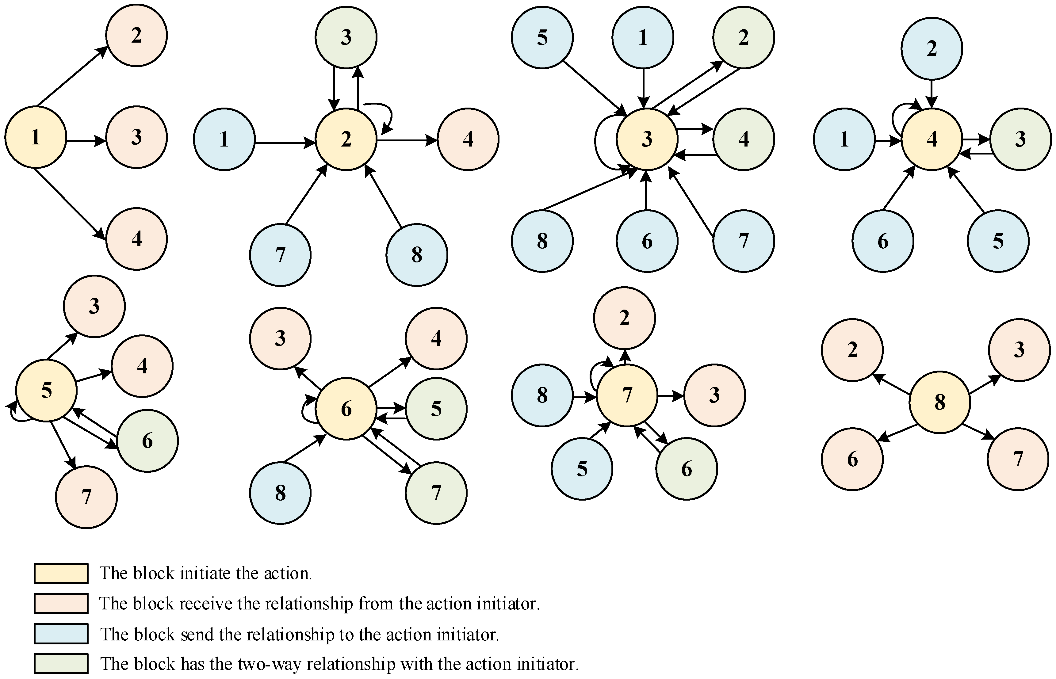
According to the present study [56,57], we selected 3 indicators representing each point network’s characteristics: degree centrality ($DC$), betweenness centrality ($BC$), and closeness centrality ($CC$). If more provinces have a relationship with the area, the degree of centrality will be higher. Betweenness centrality indicates the position of the province in the AGTFP network. Those regions located in the shortest connection path between two provinces had a higher betweenness centrality value. Closeness centrality indicated the communication level between 2 provinces. A higher value in closeness centrality indicated that a province is closer to other provinces. We also present the calculation equations of the point network in Table 1.

3.3.4. Block Model

To explore further the spatial relationships of the provinces in the AGTFP network, we utilized the block model to cluster the individuals of the network [58]. Generally, the method of CONCOR is often used to cluster and partition the spatial correlation network. The individuals were classified into 4 types of blocks: (1) net beneficial block (in which it is evident that the received connections are more significant than those sent to external blocks), (2) net spillover block (in which the spillover connections within the blocks and the provinces in the entire block are relatively more significant than those from external blocks), (3) two-way spillover block (which displays many spillover connections within and with external blocks), and (4) broker block (which commonly acts as a mediator to connect provinces, receiving and sending connections to the external provinces). In particular, we divided the nodes into four blocks based on their actual and expected internal relationships [56]. The actual internal relationship represents the ratio of blocks receiving external connections and not receiving external connections. Meanwhile, the expected internal relationships indicate the proportion of members within the block with less than half of their connections or more than half being transmitted to others within the block. In detail, the proportion of actual internal relationships = number of internal relationships of blocks/total number of spillover relationships of blocks, and the proportion of expected internal relationships = (number of provinces within the block − 1)/(number of provinces in the network − 1).

3.3.5. QAP Analysis

Compared with traditional regression, the method of QAP has the advantage of exploring the relationship using relational data [59] and dealing with multicollinearity and structural autocorrelation [60,61,62]. Hence, we utilized the QAP method to analyze the correlation between the matrices of influencing factors and the AGTFP network matrix to find the external factors for strengthening the AGTFP network. QAP analysis contains two parts: correlation analysis and regression analysis. The first part analyzes the correlation between each external factor and the AGTFP network. The second part permutates the rows and columns of an explained matrix, recomputing the regression many times (2000 times in this study) to evaluate the standard errors [59]. The simple form of the QAP model is shown in Equation (3):

$$Q=f\left(X_1,X_2,\cdots ,X_n\right)$$

(3)

where $Q$ is the spatial association matrix of AGTFP, and $X_q\left(q=1,2,\cdots ,n\right)$ represents the matrix of influencing factors.

3.4. Variables

3.4.1. Variables for AGTFP Measurement

Referencing Tian and Wu [63] and the characteristics of agriculture, we selected the following variables for inputs: traditional agricultural production input (labor, land, and capital), modern agricultural production input (energy), and natural environmental input (water resources and climatic factors). In addition, we used the total production value of agriculture as the desired output and the 2 variables of agricultural CO₂ and non-point source pollution as the undesired outputs. The details of the input–output variables are presented in

Table 2. Index description of the input–output variable.

Category	Variables	Index	Abbreviation	Unit
Input	Labor force	Number of employees in agriculture, forestry, animal husbandry, and fisheries	Labor	10,000 people
Input	Cultivated land	Crop sown area and aquaculture area	Land	1000 hectares
	Agricultural capital	Total power of agricultural machinery	Machine	100,000 kilowatts
		The pure application amount of agricultural chemical fertilizer	Fertilizer	tons
	Agricultural capital	Pesticide usage	Pesticide	tons
		Agricultural film usage	Film	tons
	Energy consumption	Agricultural diesel consumption	Diesel	tons
		Agricultural electricity consumption	Electricity	Kwh
	Water resource	Agricultural water consumption	Water	100 million cubic meters
	Climatic factors	Average temperature	Temperature	Celsius
		Precipitation	Precipitation	mm
Output	Desirable output	The gross output value in the industry of agriculture, forestry, animal husbandry, and fishery	Agricultural output	100 million CNY
	Undesirable output	Agricultural CO2	CO2	tons
		Non-point source pollution	NSP	million cubic meters

.

Here, we introduce the calculation method for the 2 undesirable variables.

Agricultural CO₂. According to the current literature [64,65,66], we selected 5 primary sources of agricultural CO₂: (1) agricultural energy consumption, (2) agricultural land utilization, (3) rice planting, (4) ruminant breeding, and (5) straw burning. We calculated the agricultural CO₂ using the activity data and emission factor based on the method provided by the IPCC; the detailed measurement is as follows:

$$E={\displaystyle \sum _{i=1}^n{E}_i}={\displaystyle \sum _{i=1}^n{T}_i}\cdot {\delta }_i$$

(4)

where $E$ is the total quantity of agricultural CO₂, $E_i$ is the quantity of CO₂ of each category of carbon source, $T_i$ denotes the amount of carbon emission source, and ${\delta }_i$ represents the carbon coefficient of each carbon source.

Agricultural non-point source pollution. Most research uses the inventory analysis method proposed by Lai [67] to measure this. Generally, there are 5 sources of non-point pollution: (1) fertilizer, (2) livestock and poultry, (3) crops, (4) aquaculture, and (5) population. The detailed measurement is shown in Equation (5):

$$E_j={\displaystyle \sum _{i=1}^{n}E{U}_i{\rho }_{ij}\left(1-{\eta }_i\right)C_{ij}\left(E{U}_{ij},S\right)={\displaystyle \sum _{i=1}^{n}P{E}_{ij}}}\left(1-{\eta }_i\right)C_{ij}\left(E{U}_{ij},S\right)$$

(5)

where $E_j$ is the quantity of the pollution $j$; $E{U}_i$ is the statistic value of the unit $i$; ${\rho }_{ij}$ denotes the pollutant production intensity coefficient of pollutant $j$ in the unit $i$; ${\eta }_i$ reflects the coefficients of the related resources usage efficiency; $P{E}_{ij}$ is the quantity of pollutant $j$; and $C_{ij}$ denotes the emission coefficient of pollutant $j$ in the unit $i$, which is determined by the characteristics of the unit and space, representing the aggregate impact of environment, precipitation, etc., in each province.

The statistical description of the input and output variables is presented in

Table 3. Statistical description of the input–output variable.

Index	N	Mean	Std. Dev	Min	Max
Labor	589	920.2843	679.4338	8.1100	3398.0000
Land	589	5413.4640	3801.7480	90.5503	15,170.1000
Machine	589	2871.1170	2740.5280	93.9700	13,353.0000
Fertilizer	589	173.2094	140.3996	3.0000	716.0900
Pesticide	589	2234.6510	12,155.4400	0.0596	114,311.0000
Film	589	70,213.7000	64,678.3000	441.0000	343,524.0000
Diesel	589	63.3613	65.0345	0.8000	487.0000
Electricity	589	224.1442	355.0139	0.4000	2011.0000
Water	589	119.6723	101.0228	3.2000	561.7470
Temperature	589	76.7005	42.7997	8.0321	195.5500
Precipitation	589	12.7821	6.1912	−1.9000	25.6770
Agricultural output	589	2522.1720	2199.3990	55.9000	10,190.6000
CO2	589	926.9984	757.4488	37.3114	8788.6030
NSP	589	45,196.0400	35,964.1900	254.0410	192,384.0000

.

3.4.2. Variables for QAP Analysis

To strengthen the AGTFP network for realizing the coordinated development of agriculture, we selected the variables of transportation development gap, technological progress gap, government support level gap, and agricultural industry structure similarities to analyze the driving factors; the detailed influencing factors are as follows (see Figure 3):

Transportation Development Gap

Transportation plays a vital role in agricultural production [68,69,70]. With transportation development, more redundant labor forces in agriculture can be transferred to cities [71], and more technical specialists can access rural areas to guide agricultural production, promoting agricultural productivity. However, when the geographical barriers are lowered because of transportation development, more people will transfer to the developed areas and inhibit the development of local agriculture. Thus, the decreased gap of accessibility between 2 regions with enormous economic development gaps will weaken the AGTFP network.

In addition, the decreased transportation cost also promotes more perishable agricultural goods being transmitted to cities, resulting in increased demand for agricultural products and stimulating agricultural productivity [55,72]. However, cargo movement will become more challenging if the 2 areas have a massive transportation development gap. Therefore, the significant difference in the cargo transportation capacity of the 2 regions will significantly weaken the agricultural product trade connections between them and further undermine the relationships within the AGTFP network.

Considering the different mechanisms of population flow and cargo movement, we selected 2 variables to reflect the level of transportation development:

• Transportation accessibility gap ($access$). The variable of transportation accessibility is frequently used to reflect transportation development and is an excellent indicator of population flow. In this study, we utilized the weighted average travel time proposed by Diao [73] to measure transportation accessibility. The specific calculation method is as follows:

  $$acces{s}_{it}=\frac{{\displaystyle \sum _{j=1}^n{M}_{jt}{T}_{ijt}}}{{\displaystyle \sum _{j=1}^n{M}_{jt}}},M_{jt}=\sqrt{PO{P}_{jt}\times GD{P}_{jt}}$$

  (6)

where $acces{s}_{it}$ represents the weighted average travel time of a city $i$ in a year $t$; $T_{ijt}$ denotes the shortest travel time from city $i$ to $j$; $PO{P}_{jt}$ and $GD{P}_{jt}$ are the population and total gross domestic production in the city $j$, respectively. We used the data of the provincial capital’s city to calculate the transportation accessibility in each province.

• Freight turnover gap ($freight$). The freight volume of each province and city reflects the connection of agricultural products between regions and cities.

Technological Progress Gap

Generally, most scholars consider technological progress to be the most critical factor for promoting AGTFP [14,74]. Energy-saving technology can increase agricultural production with less energy consumption and carbon emissions [14]. Meanwhile, promoting technological progress can support the development of modern agriculture, which could improve agricultural productivity to some extent [75,76]. However, if 2 regions have similar technological progress levels, technology transfer will become more complicated, causing weak connections in the AGTFP network:

• Energy-saving technology-level gap ($tech$). The ratio of agricultural added value in agricultural carbon emissions was used to calculate the level of energy-saving technology.
• The total quantity of patent gap ($patent$). The number of patents is widely used to represent the innovation or technology level of an area; thus, we selected the quantity of three types of patents (invention patents, utility model patents, and design patents) to reflect a region’s technology level.

Government Support Gap ($govern$)

Agriculture is a sector that is at high risk of being affected by climate change [11]; thus, support from the government is essential. Further, areas suitable for agricultural production lack economic development, so government subsidy represents a vital source for them to input into agricultural production [77]. The considerable government support gap means that the government has paid more attention to developing regions which intend to achieve the goal of coordinating regional agriculture development. Therefore, an increased government support gap will enhance the AGTFP network. To reflect the level of government support for agriculture, we chose the proportion of expenditure on agriculture, forestry, and water affairs in each province and city to general budget expenditure.

Income Gap ($pincome$)

The rural income per capita variable is a significant indicator of economic development level. Generally, 2 regions will have a stronger desire to connect if they have similar economic development levels. Therefore, narrowing the rural residents’ income gap could strengthen regional relationships and enhance the AGTFP network [55]. In this study, we selected per capita disposable income of rural residents to calculate the income gap.

Agricultural Industry Structure Similarities ($asi$)

Generally, if 2 regions have different agricultural industry structures, they will have more desire to connect to exchange various agricultural products. Further, with their relationship becoming closer, these regions will have a strong desire to realize specialized agricultural production, which could continue to promote their agricultural productivity. Thus, a great difference in agricultural industry structure could strengthen the AGTFP network. According to He et al. [54], the measurement of agricultural industry structure similarities is presented in Equation (7):

$$as{i}_{ik}=\frac{{\displaystyle {\sum }_{j=1}^n{S}_{ij}{S}_{kj}}}{\sqrt{{\displaystyle {\sum }_{j=1}^n{S}_{ij}^2{\displaystyle {\sum }_{j=1}^n{S}_{kj}^2}}}}$$

(7)

where $as{i}_{ik}$ represents the similarities of agricultural industry structure between the region $i$ and $k$; $S_{ij}$ and $S_{kj}$ denote the proportion of the agricultural industry $j$ in the gross output in the agricultural sector of the area $i$ and $k$; and $n$ is the number of subindustries in agriculture.

3.4.3. Data Source

The relevant agricultural input and output data were sourced from the China Agricultural Statistical Yearbook (2001–2020). The data on the relevant variables of QAP analysis were collected from the China Regional Statistical Yearbook (2001–2020). In addition, the data on transportation development were sourced from the China Transportation Statistical Yearbook (2001–2020).

4. Results Analysis

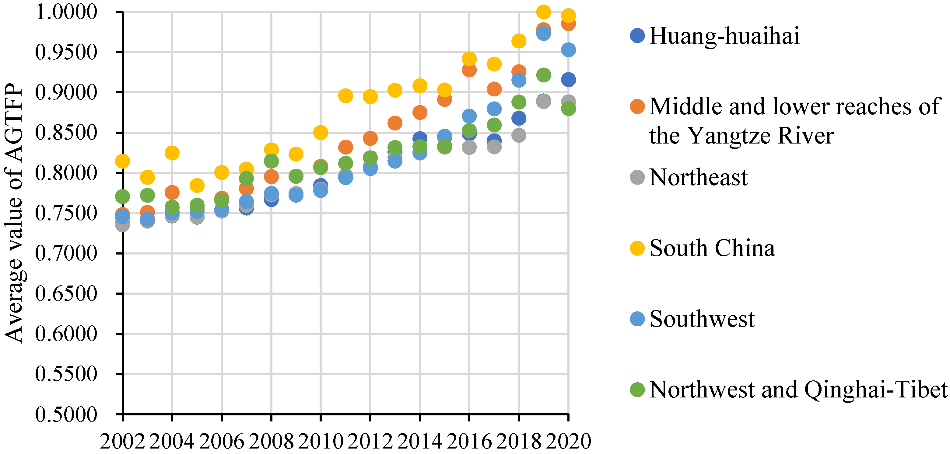
4.1. Characteristics of AGTFP Trend

According to the agricultural production input and output data of 31 provinces in China from 2002 to 2020, we calculated AGTFP using the EBM-DEA model. Overall, AGTFP increased from 0.75 in 2002 to 0.90 in 2020, indicating that the green productivity of agriculture was becoming increasingly efficient during this period (see Figure 4).

Due to each region’s geographical and economic heterogeneity in China, we also analyzed the trend of six agricultural production areas. Figure 5 shows that the average AGTFP level was highest in South China. There were some fluctuations during 2002~2010, but the general trend was upward. After 2010, the average value of AGTFP in South China was over 0.85, reaching almost 1.00 in 2019. Although the proportion of agriculture production in GDP is small in this region, its developed secondary industry could provide more advanced immediate input in agricultural production. The value of AGTFP has ranked the second highest in the middle and lower reaches of the Yangtze River since 2011, and the AGTFP in this region increased from 0.83 in 2011 to 0.98 in 2020. This region’s economic development level is exceptionally high; thus, advanced technology can continuously promote its AGTFP. After this region, the value was the third highest in Southwest China in 2020, reaching about 0.95. Southeast China is the main traditional agricultural production area. This area has substantial comparative advantages in grain production. Specialized production and industrial structure adjustment also continuously promote improving local agricultural green production efficiency.

The average value of AGTFP in the Huang-Huaihai, Northeast, Southwest, and Qinghai–Tibet area was around 0.90 in 2020, indicating a slower increase in AGTFP. These areas possess certain agricultural production advantages. For example, the Northeast area is China’s central granary, and the Southwest and Qinghai–Tibet regions have natural pastures suitable for developing animal husbandry. However, because of the relative lack of economic development in these areas, the lack of advanced production technology leads to low efficiency. Meanwhile, large-scale production also exerts more agricultural pollution on the environment, leading to the AGTFP rising slowly.

To acknowledge the apparent trend of each province, we plotted a heat map of AGTFP from 2002 to 2020 in Figure 6. Overall, the AGTFP in most of the regions in China experienced a continuous rise. The value of AGTFP was more than 0.80 after 2011 in almost half of the provinces in China. However, AGTFP fluctuated greatly in the provinces of Tibet and Hainan. In 2002, the AGTFP value of these two areas was close to one. In 2005, it dropped to below 0.80 and then increased. Agricultural production is greatly influenced by natural weather. These two areas have a low economic development level, and their ability to cope with weather changes is insufficient, resulting in large fluctuations in green agricultural productivity.

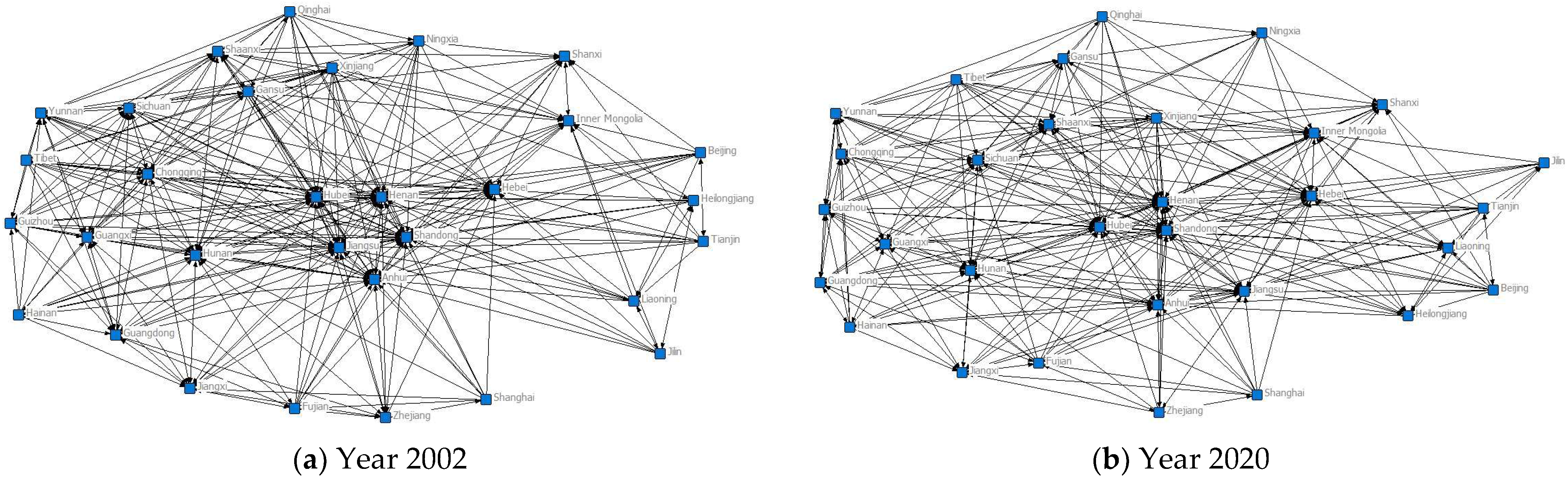
4.2. Characteristics of the Overall Social Network of AGTFP

SNA is a method frequently utilized to explore the relationships between nodes in a social network. We first constructed the gravity model to identify the spatial correlation of AGTFP among 31 provinces in China. Figure 7 presents the spatial correlation of a complex network in 31 provinces in China. We also calculated the density, connectedness, hierarchy, and efficiency to determine the overall characteristics of the AGTFP network.

Table 4. Characteristics of the overall network.

Year	Density	Connectedness	Hierarchy	Efficiency
2002	0.3839	1.0000	0.2364	0.4483
2003	0.3860	1.0000	0.2364	0.4437
2004	0.3817	1.0000	0.2364	0.4460
2005	0.3817	1.0000	0.2364	0.4529
2006	0.3796	1.0000	0.2364	0.4552
2007	0.3763	1.0000	0.2353	0.5287
2008	0.3817	1.0000	0.2364	0.4552
2009	0.3785	1.0000	0.2364	0.4598
2010	0.3312	1.0000	0.2857	0.5678
2011	0.3753	1.0000	0.2364	0.4644
2012	0.3731	1.0000	0.2364	0.4690
2013	0.3731	1.0000	0.2364	0.4690
2014	0.3753	1.0000	0.2364	0.4690
2015	0.3753	1.0000	0.2364	0.4690
2016	0.3720	1.0000	0.2364	0.4782
2017	0.3753	1.0000	0.2364	0.4713
2018	0.3785	1.0000	0.2364	0.4644
2019	0.3785	1.0000	0.2364	0.4690
2020	0.3742	1.0000	0.2364	0.4759
Average	0.3753	1.0000	0.2389	0.4714

Data source: author’s calculation.

shows that the average network density was 0.3753 from 2002 to 2020. First, network density decreased from 2002 (0.3839) to 2010 (0.3312). Then, network density experienced an upward trend from 2011 to 2020, increasing to 0.3742. Network connectedness always equals one, indicating a stable and significant relationship of the AGTFP social network. The average value of the network hierarchy was 0.2389.

Additionally, the network hierarchy has barely changed during this period, indicating the spatial network of AGTFP has been restricted by a geographical barrier. The overall network efficiency increased slightly from 2002 to 2020. However, the network efficiency increased significantly from 2002 (0.4483) to 2010 (0.5682) and then decreased to 0.4644 in 2011. After that, the efficiency continuously improved, but the rate of increase was slight, indicating that it is essential to continue strengthening the connectivity and stability of the AGTFP network.

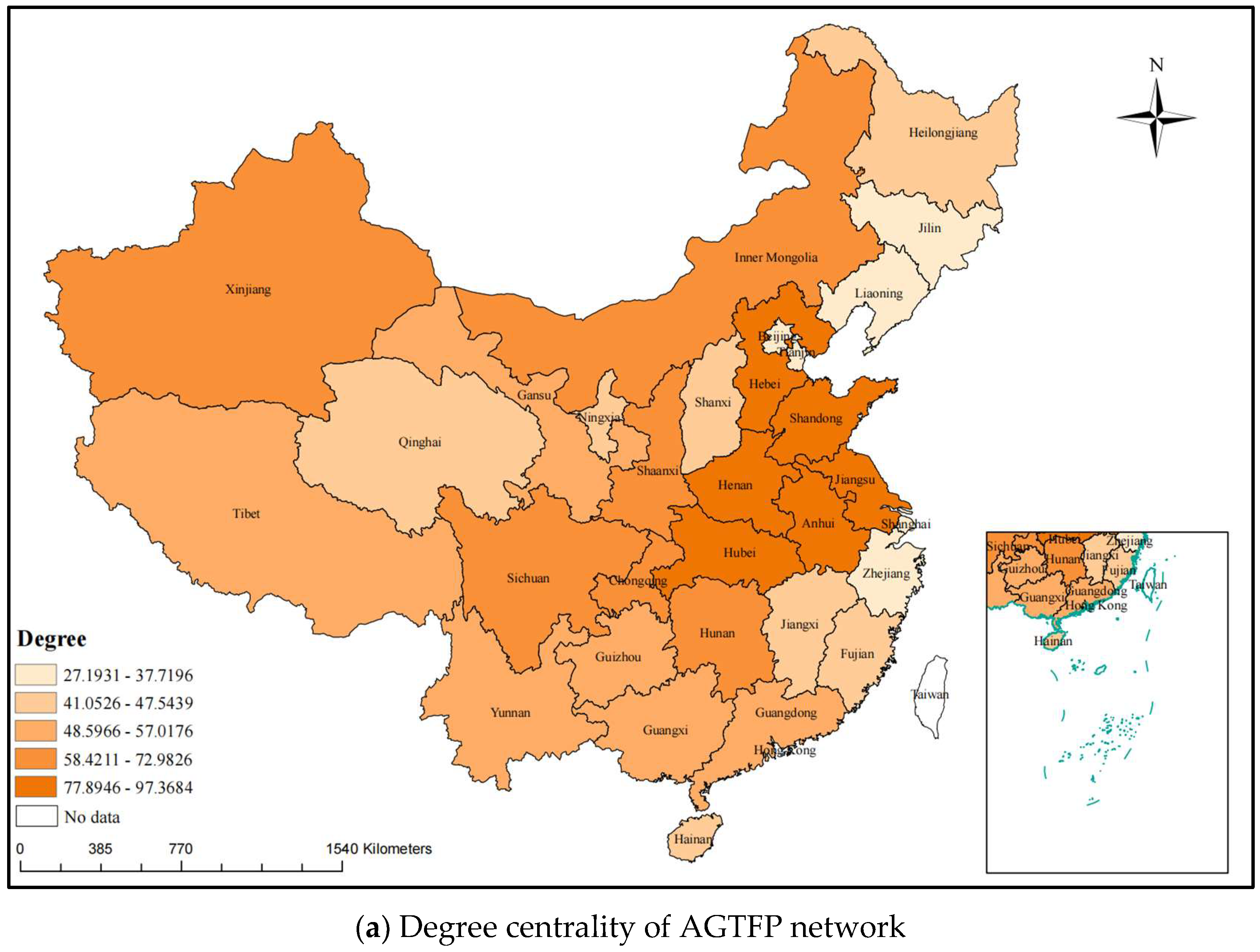
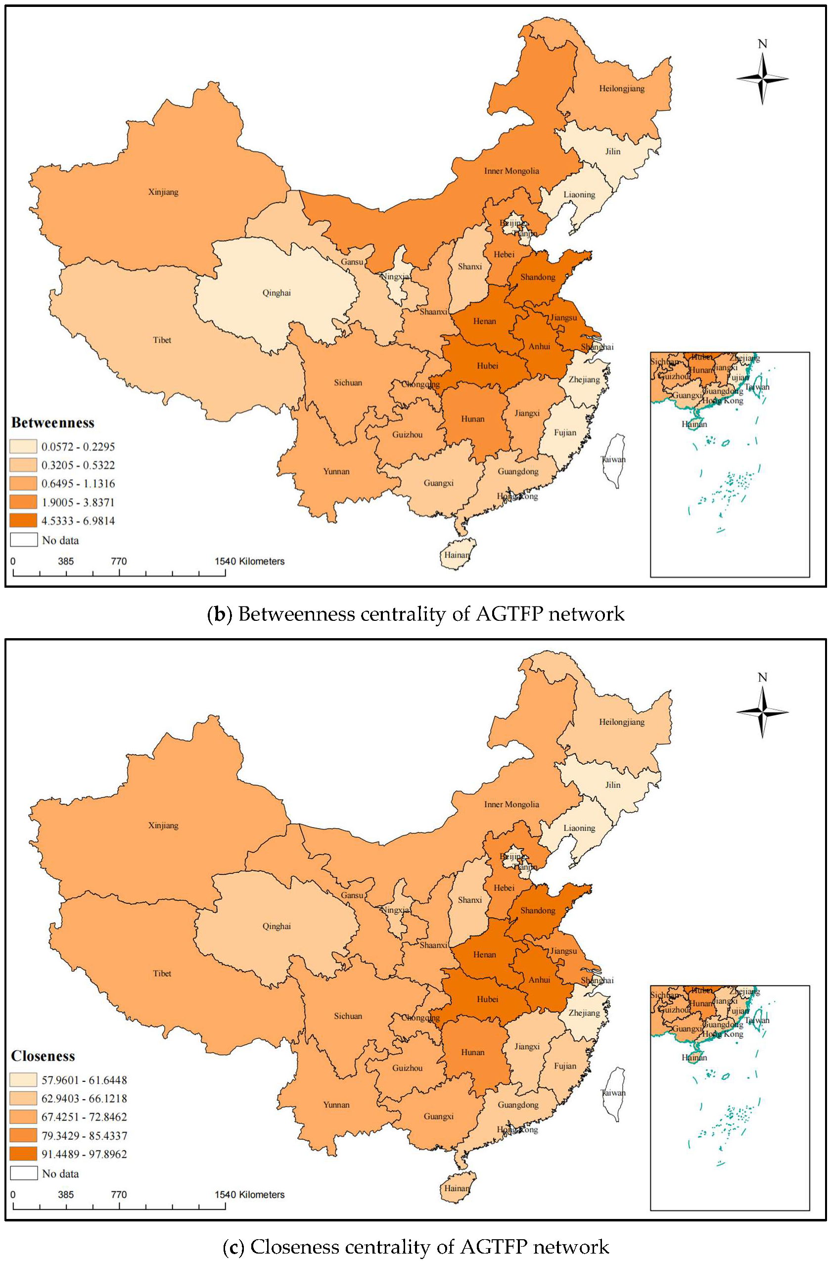
4.3. Characteristics of Point Network of AGTFP

There were three indicators selected for evaluating the role of each province in the AGTFP network: degree centrality, betweenness centrality, and closeness centrality. Figure 8 represents the spatial distribution of the centrality from 2002 to 2020. As for degree centrality, Figure 8a represents the first tier of provinces located in the central and eastern regions, such as Hebei, Shandong, Henan, Jiangsu, Anhui, and Hubei, with a degree centrality of more than 78, indicating a higher closeness relationship with other provinces. The reason for this is that they are the vital channel for connecting the southern–northern and eastern–western areas; the advantageous location allows them to exchange information through the AGTFP network. However, the degree centrality is extremely low in some large cities, such as Beijing, Tianjin, and Shanghai, and some coastal provinces, such as Zhejiang, Liaoning, and Jilin. These provinces have few connections with other nodes and are at the edge of the AGTFP network.

The top five provinces in betweenness centrality are Henan, Hubei, Jiangsu, Shandong, and Anhui (see Figure 8b). From the degree centrality analysis, one can observe that they have close connections with other provinces; thus, these areas are an essential bridge in negotiating information among provinces and can control other regions. Meanwhile, the betweenness centrality is lowest in some eastern coastal provinces, such as Liaoning, Zhejiang, etc., and some inland provinces in the west, such as Qinghai, Ningxia, etc., indicating they have a weak ability to control other areas.

Regarding closeness centrality (see Figure 8c), the provinces in the first level are Shandong, Henan, Hubei, and Anhui, indicating they are much closer to other areas in the AGTFP network, facilitating their direct relationships with other provinces, whereas while the levels of closeness centrality in Beijing, Tianjin, Jilin, Shanghai, and Zhejiang are relatively low, these provinces are situated at the edge of the AGTFP network, facilitating their control by other regions.

Overall, the centrality is highest in the central and eastern provinces such as Henan, Hubei, Shandong, Jiangsu, and Anhui. Some areas are primary agricultural production areas; they can transmit agricultural goods to other regions to construct a close relationship. Meanwhile, their location also confers an advantage; they act as an important channel to connect the northern–southern area and eastern–western area. Meanwhile, Beijing, Tianjin, Shanghai, Liaoning, Jilin, and Zhejiang have the lowest centrality at the AGTFP network’s edge. Some of them are modern cities which are weak in agricultural production and strongly reliant on other provinces. Moreover, some are the coastal provinces, far away from the inland areas, resulting in low centrality.

4.4. Block Model Analysis of AGTFP

The overall and point network characteristics show that the 31 provinces can be divided into various categories. We utilized the block model to explore the spatial clustering characteristics of the AGTFP network and determine the roles each position plays in the network. The 31 provinces were divided into eight blocks by using the data from 2002 to 2020 (see

Table 5. Spillover relationships analysis among blocks.

Block	Block 1	Block 2	Block 3	Block 4	Block 5	Block 6	Block 7	Block 8
Block 1	3	11	15	8	2	1	0	0
Block 2	1	8	16	8	0	0	5	0
Block 3	0	9	12	8	2	3	6	0
Block 4	1	0	12	6	4	3	0	0
Block 5	0	0	13	9	9	14	6	0
Block 6	0	0	15	6	8	20	12	0
Block 7	0	5	12	2	0	13	6	2
Block 8	0	7	16	3	0	12	12	2
Members	Beijing, Tianjin, Shanghai, Jilin	Inner Mongolia, Liaoning, Shanxi, Heilongjiang	Hebei, Hubei, Shandong, Henan	Zhejiang, Jiangsu, Anhui	Fujian, Jiangxi, Hainan, Guangdong	Guangxi, Hunan, Chongqing, Guizhou, Yunnan	Sichuan, Shaanxi, Gansu	Tibet, Qinghai, Ningxia, Xinjiang
Membership	4	4	4	3	4	5	3	4
Expected internal relationship	10%	10%	10%	6.67%	10%	13.33%	6.67%	10%
Actual internal relationship	7.5%	21.05%	30%	23.08%	17.65%	32.79%	15%	3.38%
Total connections received from other blocks	2	32	99	44	16	46	41	2
Total connections sent to other blocks	37	30	28	20	42	41	34	50
Block role	Net spillover	Two-way spillover	Net beneficial	Net beneficial	Two-way spillover	Two-way spillover	Two-way spillover	Net spillover

and

Table 6. Density and image matrixes of AGTFP network.

Block	Density
	Block 1	Block 2	Block 3	Block 4	Block 5	Block 6	Block 7	Block 8
Block 1	0.2500	0.6880	0.9380	0.6670	0.1250	0.0500	0.0000	0.0000
Block 2	0.1250	0.6670	1.0000	0.6670	0.0000	0.0000	0.4170	0.0000
Block 3	0.0000	0.5630	1.0000	0.6670	0.1250	0.1500	0.5000	0.0000
Block 4	0.0830	0.0000	1.0000	1.0000	0.3330	0.2000	0.0000	0.0000
Block 5	0.0000	0.0000	0.8130	0.7500	0.7500	0.7000	0.4170	0.0000
Block 6	0.0000	0.0000	0.7500	0.4000	0.4000	1.0000	0.8000	0.0000
Block 7	0.0000	0.4170	1.0000	0.2220	0.0000	0.8670	1.0000	0.1670
Block 8	0.0000	0.4380	1.0000	0.2500	0.0000	0.6000	1.0000	0.1670
Block	Image
	Block 1	Block 2	Block 3	Block 4	Block 5	Block 6	Block 7	Block 8
Block 1	0	1	1	1	0	0	0	0
Block 2	0	1	1	1	0	0	1	0
Block 3	0	1	1	1	0	0	1	0
Block 4	0	0	1	1	0	0	0	0
Block 5	0	0	1	1	1	1	1	0
Block 6	0	0	1	1	1	1	1	0
Block 7	0	1	1	0	0	1	1	0
Block 8	0	1	1	0	0	1	1	0

).

Block 1 consisted of four provinces: Beijing, Tianjin, Shanghai, and Jilin. The internal association coefficient was three, and Shanghai was isolated in this block (see Figure 9). This block has received two relationships from the external blocks, spilling 37 associations to others. Furthermore, the expected and actual internal association proportions were 10% and 7.5%, respectively. The spillover associations were more numerous than the received associations. Meanwhile, Figure 9 shows that Block 1 mainly sends connections to Blocks 2~4 and receives no effective connections from other blocks. Thus, we denote Block 1 as the “net spillover block”.

Block 2 contained four provinces: Inner Mongolia, Liaoning, Shanxi, and Heilongjiang. The internal relationship in this block was eight, and Inner Mongolia plays a vital role in connecting the provinces in Block 2 (see Figure 9). Block 2 received 32 connections from others, while there were 30 spillover associations. Based on these relationships, we could see that the expected and actual internal association ratios were 10% and 21.5%, respectively. This shows that the connections are very close among the block members and between the block and others. Figure 9 shows that Block 2 received influential connections from Blocks 1, 7, and 8 and sent a connection to Blocks 3 and 4. Therefore, Block 2 plays the “two-way spillover block” role, connecting different blocks.

There were also four provinces in Block 3, including Hebei, Hubei, Shandong, and Henan. The internal relationship was 12, indicating that every two regions in this block are associated (see Figure 9). Block 3 received 99 associations from external blocks and sent 28 connections to other blocks. It was calculated that the expected and actual internal relationship were 10% and 30%, respectively. Block 3 received significant connections from all blocks (see Figure 10) and sent effective associations to Blocks 2 and 4. Thus, it is evident that the accepted associations are greater than spillover associations, making this the “net beneficial block”. According to the centrality analysis in Section 4.3, these four provinces have the highest betweenness and closeness centrality, essential in connecting northern–southern and eastern–western areas.

Block 4 included only three provinces: Zhejiang, Jiangsu, and Anhui. The internal relationship was six, meaning all regions were connected (see Figure 9). According to the statistics, the block received 44 connections from others and sent out 20 connections. From Figure 9, we can see that Block 4 received connections from Blocks 1 to 6 and only sent correlations to Block 3. The expected and actual internal relationship proportions were 6.67% and 23.80%, respectively. It is clear that Block 4 received more connections than it sent to others, making it a “net beneficial block”. Moreover, Jiangsu and Anhui are located in the first tier of centrality, indicating they have a close relationship with other provinces. Due to Zhejiang being adjacent to the provinces of Jiangsu and Anhui, it could receive adequate information from them.

Block 5 contained four provinces: Fujian, Jiangxi, Hainan, and Guangdong. There were nine relationships within the block, and only Fujian and Hainan had no connection (see Figure 9). The value of receiving and sending connections in this block were 16 and 42, respectively. In Figure 9, we could see that Block 5 sent correlations to Block 3~7 and received connections from Block 6. Meanwhile, the expected and actual relationship ratio was 10% and 17.65%, respectively. The close connections within the block members and between the block and external blocks resulted in “two-way spillover effects”.

The members of Block 6 were Guangxi, Hunan, Chongqing, Guizhou, and Yunnan. The number of internal relationships among these members was 20, indicating a close connection within the subnetwork. Block 6 received 46 relationships from others and sent out 41 relationships. Figure 9 shows that Block 6 sent relationships to Blocks 3~7 and received connections from Blocks 5~8. The expected and actual relationship ratios were 13.33% and 32.79%, respectively. The close relationships among the memberships and with other blocks make it the “two-way spillover block”.

Block 7 consisted of Sichuan, Shannxi, and Gansu, with 6 internal relationships, 41 received connections, and 34 sent connections. In Figure 9, Block 7 received connections from Blocks 5~8 and sent connections to Blocks 2 and 3. The expected proportion of the internal relationships was 6.67%, whereas the internal relationship ratio was 15%. Considering the close relationship within the block and the connections with other blocks, we denote this block as a “two-way spillover block”.

Block 8’s members were Tibet, Qinghai, Ningxia, and Xinjiang. The internal relationship was only two: "Qinghai→Ningxia” and “Xinjiang→Tibet”. The number of received connections was 2, and the number of sending relationships were 50, mainly sent to Blocks 2, 3, 6, and 7. The expected proportion of internal relationships was 10%, whereas the internal relationship proportion was only 3.38%. The number of connections transmitted was greater than the number of connections received; thus, Block 8 is a “net spillover block”.

In conclusion, there are two “net spillover blocks,” Blocks 1 and 8. However, the reasons that they exert these effects are quite different. Block 1 is located in the east of China. Most cities in this region are modern cities such as Beijing, Tianjin, and Shanghai. Agriculture production is not the dominant industry in this region. Thus, it imports agricultural goods from the surrounding areas such as Hebei, Shandong, Henan, etc. However, Block 8 is located in the southwest and Qinghai–Tibet regions. Most of them have an advantage in agriculture but a low economic development level, leading to the import of intermediate products, machines, and technology from other provinces.

Moreover, there were two “net beneficial blocks”: Block 3 and Block 4. Most of the area in these two blocks is located in central and eastern China. Their relationships with other provinces, such as Hebei, Hubei, Shandong, etc., are close. These provinces play an essential role in connecting the areas of China.

4.5. Influencing Factors of AGTFP Social Network

Table 7. Correlation analysis of AGTFP network and influencing factors’ matrices in China.

Variable	2002	2005	2008	2011	2014	2017	2019	2020
access	0.3220 ***	0.3400 ***	0.3330 ***	0.3270 ***	0.3230 ***	0.3050 ***	0.3030 ***	0.2900 ***
tech	−0.0630	−0.0980	−0.1330 *	−0.1360 *	−0.1120	−0.0720	−0.0510	−0.0500
govern	0.0200	−0.0650	0.1080	0.0150	0.0240	0.0480	0.1200 *	0.0900
freight	−0.2970 ***	−0.3010 ***	−0.3950 ***	−0.4090 ***	−0.3420 ***	−0.3380 ***	−0.3370 ***	−0.3080 ***
pincome	0.0150	0.0150	0.0200	0.0460	0.0290	0.0580	0.0600	0.0630
patent	−0.0520	−0.0590	−0.0980	−0.1360 *	−0.0940	−0.0640	−0.0640	−0.0760
asi	0.2410 ***	0.2480 ***	0.2320 ***	0.2720 ***	0.2810 ***	0.2830 ***	0.2540 ***	0.2270 ***

Note: * p < 0.1, *** p < 0.01.

represents the QAP correlation analysis results. It shows that the variable of transportation accessibility and similarity of the agricultural structure positively correlates with the AGTFP network matrix (p < 0.01). Meanwhile, the relationship between freight turnover and the AGTFP network is significantly negative. The results indicate that the differences of $access$, $freight$, and $asi$ greatly influence the spatial correlations in the AGTFP network. Considering the multicollinearity between variables, we also utilized the method of QAP regression to analyze the relationships between each influencing factor and the AGTFP network matrix (see

Table 8. The QAP result of the influencing factors of AGTFP network in China.

Variable	2002	2005	2008	2011	2014	2017	2019	2020
access	0.0137 ***	0.2726 ***	0.2580	0.0677 **	0.6239 **	0.2488 *	0.2083	0.1541 **
tech	−0.0375 *	−0.1286 *	−0.1240	−0.2104	0.1054	0.0064	−0.0374	0.0125
govern	0.1157 *	−0.00001	−0.1376 *	−0.0840 **	−0.1966 *	−0.0534	−0.0651	0.0455 ***
freight	−0.3103 ***	−0.2906 ***	−0.3431 ***	−0.3568 **	−0.1122 **	−0.3124 ***	−0.3838 ***	−0.3318
pincome	0.2565 ***	0.1943 **	0.0725	0.0929	0.1046	0.0391	0.0524	0.1397
patent	0.1113	0.1146	0.0778	0.0726	−0.0278	0.1383 **	0.2038 **	0.1519 *
asi	0.2413 ***	0.2481 ***	0.2322 ***	0.2722 ***	0.2810 ***	0.2833 ***	0.2543 ***	0.2266 ***
Random Number Seed	499	499	499	499	499	499	499	499
Number of Permutations	2000	2000	2000	2000	2000	2000	2000	2000
R2	0.2350 ***	0.2460 ***	0.2660 ***	0.2590 ***	0.3040 ***	0.2470 ***	0.2360 ***	0.1940 ***

Note: The variable coefficients are standardized regression results; * p < 0.1, ** p < 0.05, *** p < 0.01.

).

It is clear that the indicators of $access$, $freight$, and $asi$ are almost always significant, but the influence exists in heterogeneity.

Firstly, except for in 2019, the $access$ coefficient was always significantly positive, showing that the considerable differences in transportation accessibility make the AGTFP network’s spatial correlations much closer. This is because the minor difference in transportation accessibility between regions leads to a more robust population flow, resulting in severe population loss in underdeveloped areas and negatively impacting the AGTFP network.

The coefficient $freight$ was always negatively significant except for in the year 2020, indicating that reduced differences in freight transportation ability will strengthen the spatial correlations of the AGTFP network. The influence mechanism is quite different than that of $access$. Improving transportation accessibility stimulates population flow; however, freight transportation ability indicates the potential of cargo flow. The slight difference in transmitting goods leads to an enlargement of the agricultural goods market, improving the AGTFP in each province and enhancing the relationship among the regions.

The coefficient $asi$ was always positively significant, indicating that a diversified agricultural industry structure will enhance the AGTFP network. A possible reason for this is that a differentiated agricultural industrial structure will promote the comparative advantages of various regions that specialize in producing agricultural products, facilitating these products’ exchange in multiple areas. Therefore, all provinces in China should continue to develop characteristic agriculture, realize specialized production, and strengthen the social network of AGTFP while improving the production efficiency of green agriculture.

We also found that the coefficient $patent$ has been positively significant since 2017, indicating that an increased technology level will strengthen the AGTFP network. A possible reason for this is that the accumulation of talents brought by regions with higher technological development levels will continuously promote the technical levels and exert a spillover effect on other areas, thereby strengthening the AGTFP network.

Finally, we found that the influence of $govern$ was heterogenous in different years. In 2002 and 2020, the greater the importance attached by the government, the more stability demonstrated by the AGTFP network. However, the influence was converse during the period of 2008~2014. A possible reason for this is that during the period of 2008~2014, the development of agriculture itself was relatively balanced. If a difference in the degree of government emphasis increased, the uneven effect among regions would be exacerbated to a certain extent. Therefore, the government must formulate corresponding support programs according to the state of agricultural production each year to balance agricultural production among regions.

4.6. Discussion

According to the above analysis of the AGTFP network characteristics and influencing factors, we provide some policy recommendations on improving the spatial association of the AGTFP among regions and realizing the sustainable development of agriculture.

First, transportation development is vital in promoting the coordinated development of green agriculture. From the analysis of the influencing factors, reducing the difference in freight turnover can improve the AGTFP network; however, narrowing the gap in transportation accessibility will weaken the spatial association of the AGTFP network. The results indicate that transportation development does help to expand the agricultural product market; however, the improvement of transportation also brings some issues, such as the loss of talent and capital, which could enlarge the development gap between regions. In particular, the block model analysis indicates that some provinces in western China, such as Xinjiang, Qinghai, and Ningxia, play the role of net spillovers in the network. Therefore, to further promote the balanced green regional agricultural, it is necessary to continue developing logistics channels to expand the agricultural product market and provide more support policies to the western region to attract more talent and capital inflows.

Diversifying the agricultural industry structure helps enhance network connectivity. The diversification of the agricultural industry structure refers to the development of characteristic agriculture based on each region’s advantage. In particular, characteristic agriculture is a type of modern agriculture that transforms the unique, famous, and high-quality products in a region’s characteristic agricultural resource development region into typical commodities. On the one hand, specialized agricultural production in each area helps to exert a scale effect to improve their AGTFP. On the other hand, the development of characteristic agriculture also helps to promote the exchange of agricultural products between regions, and the expanded agricultural product market brings more demand for agricultural products, indirectly stimulating the increase of their own and the neighboring AGTFP.

Moreover, more significant technological differences help to improve network connections. In the existing literature, most scholars express a belief that scientific and technical progress is the main factor driving the increase of AGTFP [14,36]. The results show that to enhance the network of AGTFP, it is necessary for developed regions to promote technological innovation and then spread the advanced technology to other areas to promote the overall AGTFP. This is because more scientific and technical personnel and funds are gathered in developed regions, and innovation costs are lower, which is more conducive to technological innovation. In addition, the block analysis indicates that large cities, such as Beijing and Shanghai, have significant spatial spillover effects on surrounding provinces. Thus, it is necessary to continue increasing agricultural scientific research and development in developed areas and provide more advanced agricultural technology support for the surrounding agricultural provinces.

In addition, the government support gap is crucial for regional sustainable agricultural development. According to the previous literature, the impact of fiscal expenditure on AGTFP is uncertain. Wang et al. [20] found that agricultural fiscal expenditure negatively affected AGTFP before the reform innovation proposed in 2015. However, Deng et al. [33] found that the share of fiscal expenditure stock in agricultural output has a positive but insignificant direct effect on AGTFP. Therefore, local governments need to formulate corresponding support plans based on the development characteristics of each region in the past year to avoid ineffective investment and achieve sustainable agricultural development in the whole area.

5. Conclusions and Policy Implications

Promoting green agricultural total factor productivity (AGTFP) is a measure that is quite essential for ensuring China’s sustainable development. At the same time, with the continuous strengthening of inter-regional linkages, realizing the coordinated development of inter-regional agriculture is of great importance. Therefore, this study analyzed the characteristics of the AGTFP network and its driving factors. We first utilized the EBM-DEA model to measure AGTFP in 31 provinces of China based on the data from 2002 to 2020. Then, the method of SNA and block models were used to explore whether AGTFP has a network structure and the relationship among the regions. Subsequently, we applied the QAP method to analyze the factors that affect AGTFP network connections, providing empirical evidence for strengthening AGFTP network connections and achieving the region’s sustainable development. Overall, we reached the following central conclusions:

(1)

The overall AGTFP increased from 0.75 in 2002 to 0.90 in 2020. Regarding regions, the AGTFP level in South China was the highest, with an average value above 0.85, and it reached a fully efficient state in 2019. The AGTFP in the middle and lower reaches of the Yangtze River and Southwest China followed with average values of 0.98 and 0.95, respectively, in 2020. However, the value of AGTFP in the Huang-Huaihai, Northeast, Northwest, and Qinghai–Tibet regions was around 0.90 in 2020, and there was still room for improvement.

(2)

From 2002 to 2020, AGTFP had a complex network structure, with an average overall network density of 0.3753, a connectedness of 1, and an average network efficiency of 0.4714. In addition, some provinces located in eastern and central regions, such as Hebei, Henan, Shandong, Jiangsu, and Anhui, had high centrality and played a vital role in connecting the network. However, some large cities and coastal provinces, such as Beijing, Tianjin, Shanghai, Zhejiang, and Liaoning, had low centrality and were more easily controlled by other areas in the network.

(3)

According to the results of the block model analysis, the entire network can be divided into eight blocks. Among them are two net spillover blocks: the developed area block (Beijing, Tianjin, Shanghai, and Jilin) and the underdeveloped Northwest and Qinghai–Tibet regions (Qinghai, Ningxia, Xinjiang, and Tibet). At the same time, there are two net beneficiary blocks, and these provinces are located in the eastern and central regions with high centrality. The rest of the areas are two-way spillover blocks.

(4)

As for the results of QAP analysis, the transportation development gap, technological progress gap, and agricultural industry structure similarities are three factors that significantly impact the AGTFP network. Firstly, narrowing the gap in transportation accessibility will widen the AGTFP development gap between regions, weakening the relationship within the AGTFP network. However, the freight turnover gap reduction can benefit from strengthening the AGTFP network. Secondly, increasing differences in the technological progress gap can strengthen the AGFTP network. This may be due to the fact that technical innovation in developed regions can spill over to underdeveloped areas, thereby enhancing the interconnection between regions. Thirdly, promoting the differences in the agricultural industry structure among areas can strengthen the AGTFP network.

According to the above conclusions, we draw the following policy implications:

(1)

Strengthen technology transfer from large cities to surrounding areas. For example, Beijing, Tianjin, and Shanghai provide agricultural technology support to adjacent provinces such as Hebei, Henan, Anhui, etc. Meanwhile, the government needs to increase agricultural policy support to Northwest China and the Qinghai–Tibet region to reduce the outflow of talent and capital and improve the sustainable development of local agriculture.

(2)

Vigorously develop the construction of rural logistics infrastructure and promote transportation efficiency and the connection between regions. In addition, areas with better transportation development need to help underdeveloped regions and use their spillover effects to the neighboring provinces to achieve balanced development among regions.

(3)

All provinces should develop characteristic agricultural construction and realize specialized agricultural production according to their comparative advantages. As the differences in agricultural industry structure between regions continue to increase, the degree of richness of the agricultural product market will increase, and the interconnection between regions will become closer.

This study expands the research object to the AGTFP network, which more clearly analyzes the spatial spillover relationship between regions. The research results lay the foundation for formulating coordinated development policies among areas in China and provide specific insights for the sustainable agricultural development of other developing countries. Generally, the most crucial recommendation is that various countries’ governments clarify the significance of coordinated regional agriculture development. Then, they should adopt related policies to promote the connection between regions, such as promoting transportation construction, developing characteristic regional agriculture, providing subsidies to underdeveloped areas, etc.

References

1. Teignier, M. The role of trade in structural transformation. J. Dev. Econ. 2018, 130, 45–65. [Google Scholar] [CrossRef]
2. Shi, H.X.; Chang, M. How does agricultural industrial structure upgrading affect agricultural carbon emissions? Threshold effects analysis for China. Environ. Sci. Pollut. Res. 2023, 30, 52943–52957. [Google Scholar] [CrossRef] [PubMed]
3. Xiong, C.H.; Chen, S.; Xu, L.T. Driving factors analysis of agricultural carbon emissions based on extended STIRPAT model of Jiangsu Province, China. Growth Chang. 2023, 51, 1401–1416. [Google Scholar] [CrossRef]
4. Zhu, Y.; Huo, C.J. The impact of agricultural production efficiency on agricultural carbon emissions in China. Energies 2022, 15, 4464. [Google Scholar] [CrossRef]
5. Guo, H.; Liu, X. Time-space evolution of China’s agricultural green total factor productivity. Chin. J. Manag. Sci. 2020, 28, 66–75. [Google Scholar]
6. Lei, S.H.; Yang, X.; Qin, J.H. Does agricultural factor misallocation hinder agricultural green production efficiency? Evidence from China. Sci. Total Environ. 2023, 891, 164466. [Google Scholar] [CrossRef]
7. Liu, H.M.; Wen, S.B.; Wang, Z. Agricultural production agglomeration and total factor carbon productivity: Based on NDDF-MML index analysis. China Agric. Econ. Rev. 2022, 14, 709–740. [Google Scholar] [CrossRef]
8. Li, G.C.; Fan, L.X.; Min, R. The coordination of agricultural development with environment and resource. J. Quant. Tech. Econ. 2011, 28, 21–49. [Google Scholar]
9. Chen, Y.F.; Miao, J.F.; Zhu, Z.T. Measuring green total factor productivity of China’s agricultural sector: A three-stage SBM-DEA model with non-point source pollution and CO2 emissions. J. Clean. Prod. 2021, 318, 128543. [Google Scholar] [CrossRef]
10. Huang, X.Q.; Feng, C.; Qin, J.H.; Wang, X.; Zhang, T. Measuring China’s agricultural green total factor productivity and its drivers during 1998-2019. Sci. Total Environ. 2022, 829, 154477. [Google Scholar] [CrossRef]
11. Emerick, K.; Janvry, A.D.; Sadoulet, E.; Dar, M.H. Technological innovations, downside risk, and the modernization of agriculture. Am. Econ. Rev. 2016, 106, 1537–1561. [Google Scholar] [CrossRef]
12. Salazzo, R.; Donati, M.; Tomasi, L.; Arfini, F. How effective is greening policy in reducing GHG emissions from agriculture? Evidence from Italy. Sci. Total Environ. 2016, 573, 1115–1124. [Google Scholar] [CrossRef]
13. Guo, Z.D.; Zhang, X.N. Carbon reduction effect of agricultural green production technology: A new evidence from China. Sci. Total Environ. 2023, 874, 162483. [Google Scholar] [CrossRef]
14. Song, S.X.; Zhang, L.; Ma, Y.X. Evaluating the impacts of technological progress on agricultural energy consumption and carbon emissions based on multi-scenario analysis. Environ. Sci. Pollut. Res. 2022, 30, 16673–16686. [Google Scholar] [CrossRef]
15. Xu, B.; Lin, B.Q. Factors affecting CO2 emissions in China’s agriculture sector: Evidence from geographically weighted regression model. Energy Policy 2017, 104, 404–414. [Google Scholar] [CrossRef]
16. Lin, B.Q.; Xu, B. Factors affecting CO2 emissions in China’s agriculture sector: A quantile regression. Renew. Sustain. Energ. Rev. 2018, 94, 15–27. [Google Scholar] [CrossRef]
17. Li, M.; De Pinto, A.; Ulimwengu, J.M.; You, L.Z.; Robertson, R.D. Impacts of road expansion on deforestation and biological carbon loss in the Democratic Republic of Congo. Environ. Resour. Econ. 2015, 60, 433–469. [Google Scholar] [CrossRef]
18. Sardar, M.S.; Rehman, H.U. Transportation moderation in agricultural sector sustainability—A robust global perspective. Environ. Sci. Pollut. Res. 2022, 29, 60385–60400. [Google Scholar] [CrossRef]
19. Yu, Z.H.; Lin, Q.N.; Huang, C.L. Re-measurement of agriculture green total factor productivity in China from a carbon sink perspective. Agriculture 2022, 12, 2025. [Google Scholar] [CrossRef]
20. Wang, S.G.; Zhu, J.Y.; Wang, L.; Zhong, S. The inhibitory effect of agricultural fiscal expenditure on agricultural green total factor productivity. Sci. Rep. 2022, 12, 20933. [Google Scholar] [CrossRef]
21. Wu, J.Z.; Ge, Z.M.; Han, S.Q.; Xing, L.W.; Zhu, M.S.; Zhang, J.; Liu, J.F. Impacts of agricultural industrial agglomeration on China’s agricultural energy efficiency: A spatial econometrics analysis. J. Clean. Prod. 2020, 260, 121011. [Google Scholar] [CrossRef]
22. Xu, X.C.; Zhang, L.; Chen, L.H.; Liu, C.J. The role of soil N2O emissions in agricultural green total factor productivity: An empirical study from China around 2006 when agricultural tax was abolished. Agriculture 2020, 10, 150. [Google Scholar] [CrossRef]
23. Yin, C.J.; Gao, X. Recalculation of China’s agricultural total factor productivity with climatic factors. J. Zhongnan Univ. Econ. Law 2022, 1, 110–122. [Google Scholar]
24. Song, Y.G.; Zhang, B.C.; Wang, J.H.; Kwek, K. The impact of climate change on China’s agricultural green total factor productivity. Technol. Forecast. Soc. Chang. 2022, 185, 122054. [Google Scholar] [CrossRef]
25. Le, T.L.; Lee, P.P.; Peng, K.C.; Chung, R.H. Evaluation of total factor productivity and environmental efficiency of agriculture in nine East Asian countries. Agric. Econ. 2019, 65, 249–258. [Google Scholar] [CrossRef]
26. Li, Q.; Li, G.; Yin, C.; Liu, F. Spatial characteristics of agricultural green total factor productivity at county level in Hebei Province. J. Ecol. Rural Environ. 2019, 35, 845–852. [Google Scholar]
27. Liu, D.D.; Zhu, X.Y.; Wang, Y.F. China’s agricultural green total factor productivity based on carbon emission: An analysis of evolution trend and influencing factors. J. Clean. Prod. 2021, 278, 123692. [Google Scholar] [CrossRef]
28. Yang, F.; Xu, Z.; Zhu, Y.; He, C.; Wu, G.; Qiu, J.R.; Fu, Q.; Liu, Q. Evaluation of agricultural non-point source pollution potential risk over China with a transformed-agricultural non-point pollution potential index method. Environ. Technol. 2013, 34, 2951–2963. [Google Scholar] [CrossRef]
29. Gong, B. Agricultural reforms and production in China: Changes in provincial production function and production in China: Changes in provincial production function and productivity in 1978-2015. J. Dev. Econ. 2018, 132, 18–31. [Google Scholar] [CrossRef]
30. Benedetti, I.; Branca, G.; Zucaro, R. Evaluating input use efficiency in agriculture through a stochastic frontier production: An application on a case study in Apulia (Italy). J. Clean. Prod. 2019, 236, 117609. [Google Scholar] [CrossRef]
31. Emrouznejad, A.; Yang, G.L. A framework for measuring global Malmquist-Luenberger productivity index with CO2 emissions on Chinese manufacturing industries. Energy 2016, 115, 840–856. [Google Scholar] [CrossRef]
32. Liu, Y.; Feng, C. What drives the fluctuations of “green” productivity in China’s agricultural sector? A weighted Russell directional distance approach. Resour. Conserv. Recycl. 2019, 147, 201–213. [Google Scholar] [CrossRef]
33. Deng, H.Y.; Zheng, W.Y.; Shen, Z.Y.; Štreimikienė, D. Does fiscal expenditure promote green agricultural productivity gains: An investigation on corn production. Appl. Energy 2023, 334, 120666. [Google Scholar] [CrossRef]
34. Luo, J.L.; Huang, M.M.; Hu, M.J.; Bai, Y.H. How does agricultural production agglomeration affect green total factor productivity?: Empirical evidence from China. Environ. Sci. Pollut. Res. 2023, 30, 67865–67879. [Google Scholar] [CrossRef]
35. Wang, G.M.; Salman, M. The driving influence of multidimensional urbanization on green total factor productivity in China: Evidence from spatiotemporal analysis. Environ. Sci. Pollut. Res. 2023, 30, 52026–52048. [Google Scholar] [CrossRef]
36. Deng, H.Y.; Jing, X.N.; Shen, Z.Y. Internet technology and green productivity in agriculture. Environ. Sci. Pollut. Res. 2022, 29, 81441–81451. [Google Scholar] [CrossRef]
37. Shen, Z.Y.; Wang, S.K.; Boussemart, J.P.; Hao, Y. Digital transition and green growth in Chinese agriculture. Technol. Forecast. Soc. Chang. 2022, 181, 121742. [Google Scholar] [CrossRef]
38. Yang, H.; Wang, X.X.; Bin, P. Agriculture carbon-emission reduction and changing factors behind agricultural eco-efficiency growth in China. J. Clean. Prod. 2022, 334, 130193. [Google Scholar] [CrossRef]
39. Yu, D.S.; Liu, L.X.; Gao, S.H.; Yuan, S.Y.; Shen, Q.L.; Chen, H.P. Impact of carbon trading on agricultural green total factor productivity in China. J. Clean. Prod. 2022, 367, 132789. [Google Scholar] [CrossRef]
40. Wang, J.J.; Zhou, F.M.; Chen, C.; Luo, Z.H. Does the integration of agriculture and tourism promote agricultural green total factor productivity? Front. Environ. Sci. 2023, 11, 1164781. [Google Scholar] [CrossRef]
41. Xu, P.; Jin, Z.H.; Ye, X.X.; Wang, C. Efficiency measurement and spatial spillover effect of green agricultural development in China. Front. Environ. Sci. 2022, 10, 909321. [Google Scholar] [CrossRef]
42. Zhou, S.; Xu, Z.W. Energy efficiency assessment of RCEP member states: A three-stage slack based measurement DEA with undesirable outputs. Energy 2022, 253, 124170. [Google Scholar] [CrossRef]
43. Muhammad, S.; Pan, Y.C.; Agha, M.H.; Umar, M.; Chen, S.Y. Industrial structure, energy intensity and environmental efficiency across developed and developing economies: The intermediary role of primary, secondary and tertiary industry. Energy 2022, 247, 123576. [Google Scholar] [CrossRef]
44. Sharma, S.; Majumdar, K. Efficiency of rice production and CO2 emissions: A study of selected Asian countries using DDF and SBM-DEA. J. Environ. Plan. Manag. 2021, 64, 2133–2153. [Google Scholar] [CrossRef]
45. Tone, K. A slacks-based measure of efficiency in data envelopment analysis. Eur. J. Oper. Res. 2001, 130, 498–509. [Google Scholar] [CrossRef]
46. Tone, K.; Tsutsui, M. An epsilon-based measure of efficiency in DEA a third pole of technical efficiency. Eur. J. Oper. Res. 2010, 207, 1554–1563. [Google Scholar] [CrossRef]
47. Zhao, P.J.; Zeng, L.G.; Li, P.L.; Lu, H.Y.; Hu, H.Y.; Li, C.M.; Zheng, M.Y.; Li, H.T.; Yu, Z.; Yuan, D.D.; et al. China’s transportation sector carbon dioxide emissions efficiency and its influencing factors based on the EBM DEA model with undesirable outputs and spatial Durbin model. Energy 2022, 238, 121934. [Google Scholar] [CrossRef]
48. Wu, P.; Wang, Y.Q.; Chiu, Y.H.; Li, Y.; Lin, T.Y. Production efficiency and geographical location of Chinese coal enterprises—Undesirable EBM DEA. Resour. Policy 2019, 64, 101527. [Google Scholar] [CrossRef]
49. Luo, Y.S.; Lu, Z.N.; Wu, C. Can internet development accelerate the green innovation efficiency convergence: Evidence from China. Technol. Forecast. Soc. Chang. 2023, 189, 122352. [Google Scholar] [CrossRef]
50. Dong, J.; Li, C.B. Structure characteristics and influencing factors of China’s carbon emission spatial correlation network: A study based on the dimension of urban agglomerations. Sci. Total Environ. 2022, 853, 158613. [Google Scholar] [CrossRef]
51. Sarkar, A.; Azim, J.A.; Asif, A.A.; Qian, L.; Peau, A.K. Structural equation modeling for indicators of sustainable agriculture: Prospective of a developing country’s agriculture. Land Use Policy 2021, 109, 105638. [Google Scholar] [CrossRef]
52. Chen, Z.; Sarkar, A.; Rahman, A.; Li, X.J.; Xia, X.L. Exploring the drivers of green agricultural development (GAD) in China: A spatial association network structure approaches. Land Use Policy 2022, 112, 105827. [Google Scholar] [CrossRef]
53. Fraccascia, L.; Giannoccaro, I. What, where, and how measuring industrial symbiosis: A reasoned taxonomy of relevant indicators. Resour. Conserv. Recycl. 2020, 157, 104799. [Google Scholar] [CrossRef]
54. He, Y.Q.; Lan, X.; Zhou, Z.; Wang, F. Analyzing the spatial network structure of agricultural greenhouse gases in China. Environ. Sci. Pollut. Res. 2020, 28, 7929–7944. [Google Scholar] [CrossRef]
55. Ji, X.Q.; Zhang, Y.S. Spatial correlation network structure and motivation of carbon emission efficiency in planting industry in the Yangtze River Economic Belt. J. Nat. Resour. 2023, 38, 675–693. [Google Scholar] [CrossRef]
56. Xu, H.C.; Li, Y.L.; Zheng, Y.J.; Xu, X.B. Analysis of spatial associations in the energy-carbon emission efficiency of the transportation industry and its influencing factors: Evidence from China. Environ. Impact Assess. Rev. 2022, 97, 106905. [Google Scholar] [CrossRef]
57. Dong, S.M.; Ren, G.X.; Xue, Y.T.; Liu, K. Urban green innovation’s spatial association networks in China and their mechanisms. Sustain. Cities Soc. 2023, 93, 104536. [Google Scholar] [CrossRef]
58. White, H.; Boorman, S.; Breiger, R. Social structure from multiple networks. I. Block models of roles and positions. Am. J. Sociol. 1976, 81, 730–780. [Google Scholar] [CrossRef]
59. Krackhardt, D. Predicting with networks: Nonparametric multiple regression analysis of dyadic data. Soc. Netw. 1988, 10, 359–381. [Google Scholar] [CrossRef]
60. Bai, C.Q.; Zhou, L.; Xia, M.L.; Feng, C. Analysis of the spatial association network structure of China’s transportation carbon emissions and its driving factors. J. Environ. Manag. 2020, 253, 109765. [Google Scholar] [CrossRef]
61. Dekker, D.; Krackhardt, D.; Snijders, T.A.B. Sensitivity of MRQAP tests to collinearity and autocorrelation conditions. Psychometrika 2007, 72, 563–581. [Google Scholar] [CrossRef] [PubMed]
62. Bruner, M.W.; McLaren, C.D.; Mertens, N.; Steffens, N.K.; Boen, F.; McKenzie, L.; Hasiam, S.A.; Fransen, K. Identity leadership and social identification within sport teams over a season: A social network analysis. Psychol. Sport Exerc 2022, 59, 102106. [Google Scholar] [CrossRef]
63. Tian, Y.; Wu, H.T. Research on fairness of agricultural carbon emissions in China’s major grain producing areas from the perspective of industrial structure. J. Agrotechnical Econ. 2020, 1, 45–55. [Google Scholar]
64. Li, B.; Zhang, J.B.; Li, H.P. Research on spatial-temporal characteristics and affecting factors decomposition of agricultural carbon emission in China. Chinese J. Popul. Resour. Environ. 2011, 21, 8–86. [Google Scholar]
65. Min, J.S.; Hu, H. Calculation of greenhouse gases emission from agricultural production in China. Chinese J. Popul. Resour. Environ. 2012, 22, 21–27. [Google Scholar]
66. Tian, Y.; Yin, M.H. Re-evaluation of China’s agricultural carbon emissions: Basic status, dynamic evolution and spatial spillover effects. Chin. Rural Econ. 2022, 3, 104–127. [Google Scholar]
67. Lai, S.Y.; Du, P.F.; Chen, J.N. Evaluation of non-point source pollution based on unit analysis. J. Tsinghua Univ. Sci. Technol. 2004, 44, 1184–1187. [Google Scholar]
68. Stifel, D.; Minten, B. Isolation and agricultural productivity. Agric. Econ. 2008, 39, 1–15. [Google Scholar] [CrossRef]
69. Teng, Z.Y.; Li, H. Transportation costs and agricultural mechanization. Econ. Rev. 2020, 1, 84–95. [Google Scholar]
70. Shamdasani, Y. Rural road infrastructure & agricultural production: Evidence from India. J. Dev. Econ. 2021, 152, 102686. [Google Scholar] [CrossRef]
71. Zhang, J.; Li, R.; Yu, H.B. Transportation infrastructure improvement, transfer of agricultural labor force and structural transformation. Chin. Rural Econo. 2021, 6, 28–43. [Google Scholar]
72. Gollin, D.; Rogerson, R. Productivity, transport costs and subsistence agriculture. J. Dev. Econ. 2014, 107, 38–48. [Google Scholar] [CrossRef]
73. Diao, M. Does growth follow the rail? The potential impact of high-speed rail on the economic geography of China. Transp. Res. Part A Policy Pract. 2018, 113, 279–290. [Google Scholar] [CrossRef]
74. He, P.P.; Zhang, J.B.; Li, W.J. The role of agricultural green production technologies in improving low-carbon efficiency in China: Necessary but not effective. J. Environ. Manag. 2021, 293, 112837. [Google Scholar] [CrossRef]
75. McArthur, J.W.; McCord, G.C. Fertilizing growth: Agricultural inputs and their effects in economic development. J. Dev. Econ. 2017, 127, 133–152. [Google Scholar] [CrossRef]
76. Aggarwal, S. Do rural roads create pathways out of poverty? Evidence from India. J. Dev. Econ. 2018, 133, 375–395. [Google Scholar] [CrossRef]
77. Fang, L.; Hu, R.; Mao, H.; Chen, S.J. How crop insurance influences agricultural green total factor productivity? Evidence from Chinese farmers. J. Clean. Prod. 2021, 321, 128977. [Google Scholar] [CrossRef]
Figure 1. Research framework.
Energies 16 05380 g001
Figure 2. SNA analysis procedure.
Energies 16 05380 g002
Figure 3. Influencing factors of AGTFP network.
Energies 16 05380 g003
Figure 4. Average AGTFP of 31 provinces from 2002 to 2020.
Energies 16 05380 g004
Figure 5. The trend of average AGTFP in six regions in China from 2002 to 2020.
Energies 16 05380 g005
Figure 6. Heat map of AGTFP in 31 provinces from 2002 to 2020.
Energies 16 05380 g006
Figure 7. The social network of AGTFP in the years 2002 and 2020.
Energies 16 05380 g007
Figure 8. Characteristics of point network of AGTFP (2002~2020).
Energies 16 05380 g008aEnergies 16 05380 g008b
Figure 9. Spatial relations within each block.
Energies 16 05380 g009
Figure 10. Spatial relations among the eight blocks.
Energies 16 05380 g010