Abstract
Many researchers are devoted to improving the prediction accuracy of daily load profiles, so as to optimize day-ahead operation strategies to achieve the most efficient operation of district heating and cooling (DHC) systems; however, studies on load prediction and operation strategy optimization are generally isolated, which leaves the following question: what day-head load prediction performance should be paid attention to in the operation optimization of DHC systems? In order to explain this issue, and taking an actual DHC system as a case study, this paper proposes an evaluation method for the prediction of daily cooling load profiles by considering the impact of inaccurate prediction on the operation of a DHC system. The evaluation results show the following: (1) When prediction models for daily load profiles are developed, the prediction accuracy of the daily mean load should be emphasized, and there is no need to painstakingly increase the accuracy of load profile shapes. (2) CV and RMSE are the most suitable deviation measures (compared to others, e.g., MAPE, MAE, etc.) for the evaluation of load prediction models. A prediction model with 27.8% deviation (CV) only causes a 3.74% deviation in operation costs; thus, the prediction performance is enough to meet the engineering requirements for the DHC system in this paper.
1. Introduction
Climate change and energy security are regarded as two of the main global challenges [1]. The 26th UN Climate Change Conference of the Parties (COP26) set targets for many countries in terms of energy conservation, emission reductions, and coping with climate change. The intelligent and effective use of energy is key to solving energy and environment issues. District heating and cooling (DHC) technology is regarded as a solution that can effectively reduce primary energy consumption and carbon emissions while meeting buildings’ heating and cooling demands [2]. The technical classification and development of DHC systems have been described in detail in this paper [3]. DHC systems can utilize various types of energy synthetically and improve energy efficiency, which has been confirmed in European countries. The last statistical survey on the DHC sector reported that there were about 6000 district heating (DH) systems in operation in Europe, supplying about 11–12% of total heat in 2017, and 115 district cooling (DC) systems [4].
Load prediction serves as the foundation for advanced decision making in DHC systems. Under time-of-use (TOU) prices, the operation strategies of district energy systems are generally formulated 24 h in advance, especially when energy storage systems are involved [5]. Therefore, the development of models with which to accurately predict daily load profiles is essential for district energy systems.
Numerous studies focus on load prediction models dealing with a wide range of different methods. Especially with the development of information and communications technology (ICT), data-driven prediction methods have attracted a lot of attention in recent years [6,7]. Studies on data-driven methods cover many aspects, from mathematical algorithms to data. According to the classification of mathematical algorithms, traditional statistical algorithms, decision trees, artificial neural networks (ANNs), and support vector machines (SVMs) are the most widely used prediction algorithms [8]. Common traditional statistical algorithms include multiple linear regression (MLR) [9,10], the autoregressive moving average (ARMA) model, and the autoregressive with exogenous (ARX) model [11]. Typical algorithms of decision trees include RF [12], C4.5 [13] and CART [14]. These model are generally easy to use and computationally inexpensive, but their performance is usually fair [15]. Therefore, models with which to characterize complex nonlinearities have been developed (e.g., ANNs and SVMs). In a previous paper [16], a backpropagation artificial neural network algorithm was adopted to construct an energy consumption prediction model. Dong, Cao & Lee [17] used SVMs for the first time to predict buildings’ energy consumption, and pointed out that an SVM model was superior to neural network and genetic algorithms. In recent years, more advanced mathematical algorithms for prediction have also been introduced to the public, such as deep learning [18,19] and sparse coding [20]. With regard to data aspects, types of features and data sizes are extensively analyzed. For instance, Rana et al. [21] used machine learning feature selection methods to identify a small but informative set of variables in the prediction of cooling load for commercial buildings. For new buildings or existing buildings with inadequate monitoring systems, transfer learning was used to improve load forecasting accuracy [22,23].
While there is a wide body of literature focusing on load prediction, it is usually independent from the studies on operation strategy optimization. With specific applications to develop the optimal operation strategies of complex energy systems, static loads are generally used [24]. Hu et al. [25], for example, proposed a probability-constrained multiobjective optimization model for CCHP system operation, and the hourly electric, cooling, and heating loads were obtained from a reference office building in EnergyPlus. Jing et al. [26] investigated an optimal operating strategy of a small-scale integrated energy-based district heating and cooling system. The heating and cooling loads of the building were estimated to use the load index method. Liu et al. [27] proposed a new operation strategy for CCHP systems, which is choosing EnergyPlus to simulate the energy consumption of a hypothetical hotel. The disjunction of the two steps makes it difficult to bridge the performance of load prediction and the actual energy system operation results. This being the case, there remains a key question: what performance do we expect from the prediction models in order to optimize the operation strategies?
At present, the performance of prediction models is described by some measures of prediction error, including the coefficient of variation (CV), mean absolute percentage error (MAPE), and root mean square error (RMSE). The survey results showed that about 41%, 29%, and 16% of the studies used CV, MAPE, and RMSE to evaluate their prediction models, respectively [8]. In addition, the mean absolute error (MAE), mean bias error (MBE), mean square error (MSE), and R-squared (R2) can also be used to describe the performance of prediction models; however, these indices are only applicable to the horizontal comparison of different prediction models, which cannot indicate whether a model meets the requirements of guiding optimal operation. Zhang et al. [28] counted the number of running chillers under different predicted loads as an index of prediction models in order to make the evaluation of greater practical significance. However, this is not suitable for a complex energy system (e.g., the system contains a thermal energy storage system), where prediction and operation strategy optimization should both be concerned. Therefore, an evaluation index of the prediction model, reflecting the practical impact of inaccurate loads on the optimal operation of complex energy systems, is desired.
Therefore, this study aims to evaluate daily load profile prediction by considering the practical impact of inaccurate load prediction on the operation of district energy systems. A specific DHC system with three subsystems is concerned. Four common models are developed to generate predicted daily cooling load profiles, and two deviation measures for daily load profile prediction are defined, namely the daily mean load deviation (DMLD) and daily load profile coefficient deviation (DLPCD). Then, aiming at the lowest costs, the operation strategy is optimized under the profiles of actual load and predicted load. Finally, the prediction of daily load profiles is evaluated by the deviation in operation costs.
The main contents of this paper are as follows: A brief description of the DHC system is presented in Section 2. Section 3 introduces the research method in detail, including the prediction models and strategy optimization method. Additionally, a new evaluation index is proposed. Section 4 discusses the prediction performance under different evaluation indices. Conclusions are drawn in the last section.
2. Description of the DHC System
2.1. System Configuration
The DHC system studied in this paper is located in Tianjin, China. It provides heating and cooling to six single office buildings whose total construction area is about 240,000 m2. The design load is 20,458 kW in the summer and 14,000 kW in the winter. The flow chart of the DHC system is shown in Figure 1. The basic equipment information can be found in Table 1. Since municipal heat sources are applied to heating during the winter, this paper focuses on the operation of DHC systems in summer conditions.
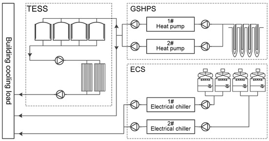
Figure 1.
The flow chart of the DHC system.

Table 1.
Basic equipment information of the DHC system.
2.2. Energy Price Policy
The time-of-use (TOU) electricity price used in the DHC system in this paper refers to the unified standard formulated by the Tianjin Price Bureau, as shown in Table 2.
Table 2.
TOU electricity price.
2.3. Cooling Load Characteristic
The operation data of hourly cooling loads are obtained from the automatic monitoring platform from 24 June 2017 to 27 August 2017, as shown in Figure 2. It is evident that the variation in the hourly cooling load corresponds with the characteristics of typical office buildings. Firstly, there are obvious load characteristic differences between working and nonworking days, namely the fact that the loads of nonworking days are much lower than those of working days. Secondly, with respect to daily load profiles (as shown in Figure 3), there are differences in the load fluctuation characteristics between working and nonworking days. On working days, the maximum load occurs at 7:00–8:00, since the system needs to cool down the indoor space and the high-temperature water in the pipelines as soon as possible when it is turned on in the morning. Subsequently, the load gradually decreases and stabilizes, and it reduces to 0 after people finish work at 17:00; however, during nonworking days, it shows a relatively stable low load characteristic.
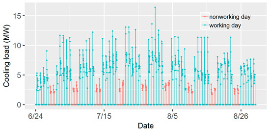
Figure 2.
The time series of the hourly cooling load.
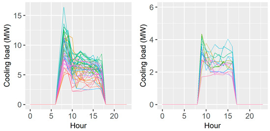
Figure 3.
The daily load profiles on a working day (left) and nonworking day (right).
According to the load characteristics mentioned above, it can be inferred that the cooling load is affected by the day types (DTs) and the variation characteristics of daily load profiles (LPs). Therefore, the day types (0 for working days, 1 for nonworking days) and the characteristic values of load profiles are supposed to be the input variables of cooling load prediction. The specific values of load profile characteristics are shown in Table 3, which are calculated with the method of min–max normalization for the average loads of working days and nonworking days. Additionally, the key factor affecting the building cooling load is the outdoor environment. Due to the limitations of data acquisition, this paper selects outdoor dry bulb temperature (DBT) and wet bulb temperature (WBT) as the two input variables of cooling load prediction, and the time series is shown in Figure 4.
Table 3.
The characteristic values of load profiles on working and nonworking days.
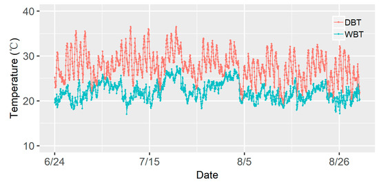
Figure 4.
Hourly outdoor dry bulb temperature (DBT) and wet bulb temperature (WBT).
3. Research Method
In combination with the practical case introduced in Section 2, this section introduces the specific research methods. Firstly, four common prediction models (MLR, CART, ANNs, and SVMs) are developed for hourly cooling load prediction 24 h in advance. Secondly, indices representing overall prediction deviations and daily prediction deviations are calculated to describe the performance of prediction models. Finally, in combination with the optimization algorithm, the optimal strategy is made and operation costs are calculated based on the actual load and the predicted load, respectively. The operation cost deviation (OCD) is calculated to reflect the influence of inaccuracy load prediction on the operation of the DHC system, which can help to evaluate the performance of prediction models with more practical significance.
3.1. Generation of Predicted Daily Cooling Load Profiles
As mentioned in a previous paper [8], data-driven prediction models, traditional statistical algorithms, decision trees, ANNs, and SVMs are often used to predict building loads. Under this model classification framework, four commonly used models are implemented to predict hourly cooling loads in this paper. MLR is specifically selected as a traditional statistical model. The classification and regression tree (CART) algorithm is selected to represent the model class of decision trees, the ANN model adopts a multilayer feed-forward network structure with a backpropagation learning algorithm, and SVMs use a Gaussian radial basis function as its kernel function. The input datasets of each prediction model include the four variables introduced in Section 2.3, which can be abbreviated as , where denotes day types, is dry bulb temperature (°C), is wet bulb temperature (°C), and denotes the characteristic values of load profiles. The specific model structures are as follows:
- Model 1: MLR
The MLR model can be described as shown in Equation (1):
where are the coefficients associated with the input variables, which can be obtained using the least-squares method, and is the output vector.
- Model 2: CART
Decision tree algorithms use a tree to map instances into predictions, being flexible algorithm that can improve themselves with an increased amount of training data. The CART, a widely used decision tree induction method, is a recursive algorithm in data mining that explores the structure of a dataset and develops decision rules for predicting dependent variables based on several independent variables. The CART uses the Gini coefficient as its classification criterion. The splitting rule in the CART is made in accordance with the squared residuals minimization algorithm, which means that the expected sum variances for two resulting nodes should be minimized. In this model, the is regarded as the dependent variable and are the independent variables. The CART algorithm is calculated by R software (R-4.3.1) in this paper.
- Model 3: ANNs
The ANN model excels at expressing arbitrary nonlinear problems, and are suitable for modeling hourly load. A very common neural network architecture is the multilayer feed-forward network with a backpropagation learning algorithm. Generally, it has three layers, including the input, output, and hidden layers. The input vectors are . The hidden layer node number is important for balancing the model complexity and accuracy, which can be determined by the method in a previous paper [29]. The detailed mathematical theory of ANNs can be simulated by R software (R-4.3.1).
- Model 4: SVMs
SVMs are kernel-based machine learning algorithms that can be used for both regression and classification. SVMs are effective at solving nonlinear problems, even with a relatively small amount of training data. In this paper, an SVM with a Gaussian radial basis function kernel is used alongside the grid search method to search for the optimal parameters, C, and kernel function radius, . The detailed introductions of the SVM algorithm can be obtained in paper [30]. The SVM model is trained with the datasets of by R software (R-4.3.1).
3.2. Measures of the Prediction Performance
In general, indices of overall prediction deviation are often used to describe the performance of a prediction model (e.g., CV and MAPE). Nevertheless, the characteristics of daily prediction deviation are different through different models (e.g., some models are good at predicting daily mean load, while others can accurately describe the variation in load profile), which should be considered to analyze the impact on the operation strategies formulated on a daily basis.
3.2.1. Deviation Measures for Prediction Models
As introduced in Section 1, seven commonly used error statistical indices are selected to evaluate overall prediction deviation. The calculation formulas are described as follows:
where is the predicted load at point , is the actual load at time , denotes the average actual load, and is the total number of data points in the dataset.
3.2.2. Deviation Measures for Daily Load Profiles
The daily predicted load can be expressed in terms of mean load and the load profile coefficient. With an accurate daily mean load and daily load profile coefficient, a good predicted load result can be guaranteed. The indices of the daily mean load deviation (DMLD) and daily load profile coefficient deviation (DLPCD) are proposed to illustrate different aspects of the prediction deviation characteristic. The calculation formulae are expressed in Equations (9)–(11):
where denotes the daily mean value of the predicted load (kW) and is the actual load (kW); the value of is 1 to 4, denoting the different models; and the value of is 1 to 5, denoting the different days.
where denotes the daily load profile coefficient, calculated by Equation (11); denotes the predicted or actual hourly load values (kW); and represents the calculation of the Pearson correlation coefficient.
3.3. Evaluation of the Prediction Performance
The purpose of load prediction is to determine the operation of a DHC system. When the predicted load deviates from the actual load, the operation strategy based on the predicted load will also differ from the one based on the actual load, resulting in operation cost deviation. Therefore, it is of more practical significance to evaluate load prediction with operation cost deviation. The analysis process is shown in Figure 5, which can be divided into two parts: firstly, the optimal operation strategies under the guidance of actual load and predicted load are obtained by using the strategy optimization method. Then, the operation costs can be simulated and calculated using the above strategies under actual load conditions, which help to calculate the operation cost deviation. A detailed calculation method is introduced in the following sections.
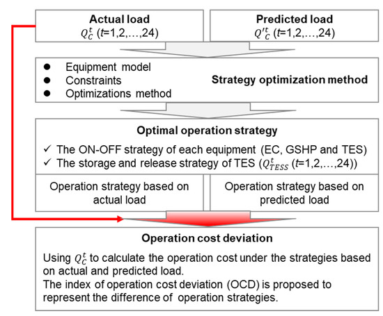
Figure 5.
The calculation process of operation cost deviation.
3.3.1. Strategy Optimization Method
Firstly, equipment models are introduced to calculate the power consumption under different load conditions. With the main objective of minimizing operation costs, general algebraic modeling system (GAMS) software is used to find optimal operation strategies based on the energy balance and equipment constraints. The GAMS is an advanced modeling system for mathematical programming and optimization. With the GAMS, the interior point method is used to solve the optimization model.
- (1)
- Equipment Models
- Electric Chiller Model
The power consumption of the electric chiller () is calculated according to the cooling capacity () and equipment efficiency (), as in Equation (12), where the can be calculated with the partial load rate () of the electric chiller and the coefficients of Equation (13) are fitted from the measured data as shown in Figure 6. (, , and .)
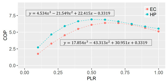
Figure 6.
The efficiency curve of the electric chiller and heat pump [31].
- Heat Pump Model
The power consumption of a heat pump () can also be obtained with its cooling capacity () and equipment efficiency () using Equations (14) and (15). Where and denote the cooling capacity supplied to buildings directly by the heat pump, is the cooling capacity supplied to the TESS. The coefficients of Equation (15) are as shown in Figure 6 (, , , and ):
- Fans and Pumps
When the electric chiller, heat pump, and TESS are running, the associated pumps and fans shown in Figure 1 are running simultaneously, and all of them operate according to the rated power (summarized in Table 1).
- (2)
- Object Function
The daily operation cost () is the object function that should be minimized in the case of optimization. It can be expressed as follows:
where is the electricity price at time and the specific values are shown in Table 2. is the total power consumption of all opened pumps, and is the total power consumption of all opened cooling tower fans.
- (3)
- Constraints
The cooling capacity of the DHC system should be equal to or greater than the cooling load of buildings, which can be expressed as follows:
where denotes the cooling capacity stored and released by the TESS. means the total cooling load (kW). The TESS meets the following energy balance:
where denotes the energy state (kW). is the heat loss of the TESS (%). is the efficiency of the TESS (%). is the rate of the TESS (%). The superscripts of and mean the energy storage and energy release of the TESS, respectively.
The outputs of the electric chiller and heat pump have following constraints:
where , , , and represent the lower and upper limits of unit output, respectively. , are the variables of 0–1, which are used to indicate the equipment conditions of ON-OFF.
Equations (13) and (15) are nonlinear expressions. In order to build a mixed-integer model, piecewise linearization is used to linearize Equations (13) and (15). The specific methods can be accessed in a previous paper (Tian et al., 2016).
3.3.2. Operation Costs under Different Load Conditions
Based on the above optimization method, the ON-OFF strategy of each equipment and strategy of the storage and release of the TESS can be obtained, which will contribute to the calculation of the operation costs. In the actual operation process, the cooling capacity of energy equipment will adjust itself (such as adjusting the chiller output according to the return water’s temperature of the system) according to the actual load demand of the buildings, which will match the cooling capacity of the DHC system with the variation in the actual load. As a result, there will not be any excessive cooling capacity even under the guidance of an inaccurate prediction load. Therefore, the operation costs are simulated under the actual load conditions. A detailed calculation process is shown in Algorithm 1.
| Algorithm 1. Calculation of operation costs |
| (1) Operation cost of HP-S can be determined through the optimization results. So the operation cost of HP-S can be calculated as: |
| (2) Operation cost of EC and HP-D The operation cost of EC and HP-D can be calculated as follows: present the rated cooling capacity of EC and HP respectively. (3) Operation cost of Fans and pumps When the EC, HP and TES are running, the associated pumps and fans are running simultaneously. So the operation cost of Fans and pumps can be calculated as follows: (4) Daily operation cost of DHC system |
| can be obtained by the ON-OFF strategy based on optimization results) |
As, in the formulation of the strategy, the goal is to minimize the total daily operation costs, it is meaningless to analyze hourly operation cost deviation. The daily operation cost deviation (DOCD) between Models 1–4 and the actual load are calculated by Equation (24):
where the value of is 1 to 4, denoting the different models, and the value of is 1 to 5, denoting the different days. In addition, the total operation cost deviation (TOCD) can be calculated as follows:
4. Results and Discussion
4.1. Performance of Load Prediction Models
The four load prediction models given in Section 3.1. are used to predict the hourly cooling load. Data from 24 June to 25 August (a total of 1488 sample points) are used to train the models. Data from 26 August to 30 August (a total of 120 sample points) are used for prediction. It can be concluded qualitatively from the hourly prediction results shown in Figure 7 that the MLR model performed badly at the start-up time (7:00–8:00), and its predicted values are far greater than the actual values. The CART model is more accurate in predicting the daily mean load, but it fails to describe the variation in hourly loads in a day. Compared with the MLR model, the ANN model can better predict start-up loads, but the overall prediction deviation on individual days is larger (e.g., on 30 August). Intuitively speaking, the SVM is the best prediction model among the four.
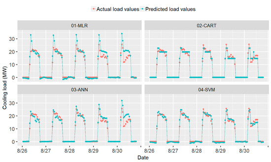
Figure 7.
The results of hourly cooling load prediction.
4.1.1. Overall Prediction Deviation
Based on the prediction results, the indices of overall prediction deviation can be calculated as shown in Table 4. From the calculation results of all of the indices, the MLR model is the worst. The prediction accuracy of the ANN model is slightly higher than that of the MLR model. The prediction performance of the CART and SVM models is much better than that of the ANN and MLR models. For the comparison of the CART and SVM models, the results are different according to different indices. The performance of the SVM model is better than that of the CART model in terms of the evaluation indices of CV, RMSE, MSE, and R2, while the CART model is better when MAPE, MAE, and MBE are used.
Table 4.
The results of the overall prediction deviation of the four prediction models.
4.1.2. Daily Prediction Deviation
The DMLD and DLPCD of four models are calculated in five days, as shown in Figure 8. Obviously, there are different deviation characteristics for different models. As for all of the generated deviation samples, some show a higher daily load prediction accuracy (i.e., lower DMLD) while having a larger deviation in their load profile shapes (i.e., higher DLPCD). On the contrary, some samples are poor in daily load prediction but accurate in load profile shape prediction. From the perspective of different prediction models (subgraph in Figure 8), the DMLD and DLPCD of the MLR model are the highest, and those of the ANN model are also higher than the CART and SVM models. Although the CART model performed worse in terms of load profile shape than the SVM model, the prediction accuracy of daily mean load of the CART model is higher.
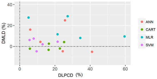
Figure 8.
The daily prediction deviation of the four models in five days (DMLD: daily mean load deviation; DLPCD: daily load profile coefficient deviation).
4.2. The Results of Optimal Operation under Different Load Conditions
4.2.1. The Operation Strategies
The operation strategies can be obtained under the load profiles in Section 4.1. using the method in Section 3.3.1. Inaccurate load will result in different operation strategies and the inefficient operation of the DHC system. The results of operation strategies on August 26th can be used as an example to clearly show the differences among strategies caused by load prediction deviation, as is shown in Figure 9. At the start-up time in the morning, the load predicted by the MLR model is much larger than actual load, so the operation strategy shows that there is one more heat pump running in the case of the MLR model than in that of actual load (AL) at 7:00, while at 8:00 and 9:00 there was an extra electricity chiller running in the MLR model. The operation strategy of the TESS also changed due to the predicted load deviation, which was embodied in the differences in the energy storage and release time of the TESS, the cooling capacity supplied by the heat pump (1# and 2# HP-S) to the TESS, and that supplied by the TESS to the buildings. The operation strategy of the TESS will affect the total operating costs of the DHC system through utilizing different TOU electricity prices.
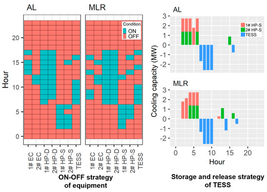
Figure 9.
The representation of operation strategy deviation (AL: actual load; MLR: multiple linear regression).
4.2.2. The Operation Costs
The hourly operation costs of the DHC system are calculated based on the different operation strategies formulated through different load conditions (actual load and predicted load). Because the predicted load deviates from the actual load, the optimized strategies will be different, which will lead to different operation costs (as shown in Figure 10). Figure 11 shows the statistical results of daily operation cost deviation (DOCD) and total operation cost deviation (TOCD) under different load conditions. Different prediction deviation characteristics may result in different operation cost deviations. Taking August 26th as an example, the MLR model predicted a load profile (daily mean load deviation: = 9.5%, daily load profile coefficient deviation: = 59.5%) with large deviation at the start-up time, which resulted in a 4.95% DOCD. The load profile shape predicted by the ANN model is relatively accurate, but the daily load is lower than the actual value ( = −5.1%, = 24.4%), and the DOCD is as high as 4.68%. The CART model predicts a nonfluctuating load profile ( = 4.1%, = 25.2%) with only a 0.67% increase in DOC. The SVM model obtains a predicted load ( = 2.0%, = 13.0%) that matches the actual load profile well, and its DOC is basically consistent with that under the actual load.
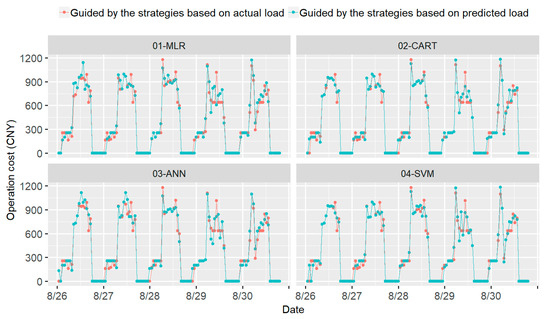
Figure 10.
The hourly operation costs of the DHC system under different load conditions.
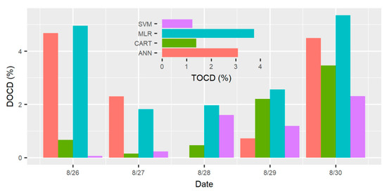
Figure 11.
The results of daily operation cost deviation (DOCD) and total operation cost deviation (TOCD).
In terms of the total operation cost deviation (TOCD) (subgraph in Figure 10), the predicted load of the SVM model has the least influence on the operation strategy of the DHC system (the TOCD is only 1.23%). The prediction performance of the CART model is close to that of the SVM model, with a 1.39% TOCD. The MLR and ANN models have poor load prediction accuracy, which results in a larger TOCD than that for the CART and SVM models. Even so, the MLR and ANN models only add 3.74% and 3.09% to the total operation costs of the DHC system.
4.3. Evaluation on Prediction Performance
Section 4.1 shows the results of prediction performance through the deviation indices. Section 4.2 shows the results of operation cost deviation under different load conditions. This section carries out the evaluation of prediction performance using operation cost deviation of the DHC system.
4.3.1. Evaluation on Predicted Daily Load Profiles
There are different daily prediction deviation characteristics (shown in Section 4.1.1), which have different influence on the operation cost of the DHC system. Such influence can be assessed by the index of DOCD. Figure 12 shows the correlation between DMLD, DLPCD and DOCD. Firstly, the predicted load-oriented operating costs are higher than actual load-oriented ones, which is reflected by the fact that all the DOCD are greater than 0. However, the deviations of the operating costs are much smaller than the deviations of load prediction. Even if the DMLD reaches 30% or the DLPCD reaches 50%, the DOCD is no more than 6%. Secondly, the DOCD is correlated with the DMLD, such as in the elliptical region in Figure 12, which denotes that the DOCD is mainly affected by the DMLD. The DLPCD does’t have strong correlation with the DOCD, and only when DLPCD exceeds 50%, will it have a great impact on the operating cost of the system (as point A in Figure 12). Finally, predicted loads lower than actual loads (DOCD is negative) are more likely to lead to changes in the operational strategy, which in turn increases operating costs. On the basis of the trends of DOCD with DMLD, with every percent of increase in DMLD, the DOCD will increase by 0.99% in negative load deviation and by 0.2% in positive load deviation, respectively.
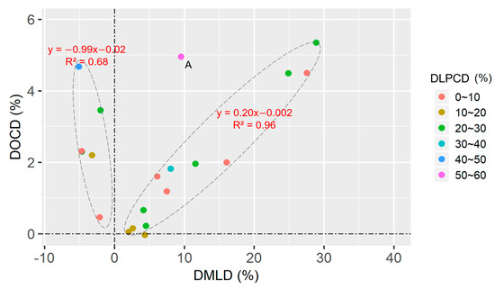
Figure 12.
The relationship of daily operation cost deviation (DCOD) with daily mean load deviation (DMLD) and daily load profile coefficient deviation (DLPCD).
4.3.2. Evaluation of Different Prediction Models
As can be seen in Section 4.1.1, there are differences in the performance ranking of prediction models with different error statistical indices. TOCD is the most suitable index to explain the impact of load prediction deviation on system operation. Therefore, the performance of four prediction models can be ranked using TOCD, as shown in Table 5. When compared with the ranking result of TOCD, the results of other error statistical indices, such as CV, RMSE, MSE, and R2, are consistent with it. The other three indices, MAPE, MAE, and MBE, are biased in their evaluations of the predicted results of the CART and SVM models.
Table 5.
The assessment of overall prediction performance.
Moreover, different indices have different ratios (). For example, compared with the MLR model, the accuracy of the CART model increased by 56.1% using the CV index, while the accuracy of the CART model increased by 80.5% using the MSE index. The matrix of Equation (26) shows that the ratios of of different indices vary significantly. In order to more accurately judge the approximation between error statistical indices and the TOCD index, the column vectors of the matrix are min–max normalized separately, as shown on the right-hand side of Equation (26). The Pearson correlation coefficients between CV, RMSE, MSE, and R2 and TOCD are then calculated to find the ones closest to the TOCD index. As shown in Table 5, the Pearson correlation coefficients of CV-TOCD and RMSE-TOCD are as high as 0.98, and the evaluation effects of CV and RMSE are slightly higher than for MSE and R2. As a result, for this case study, the CV and RMSE are the best two evaluation indices for this cooling load prediction.
When CV is chosen as the evaluation index of the prediction models, the total operation cost deviation of the DHC system is only 3.74% when the prediction accuracy is 27.8%. Additionally, the cost only deviates by 1.23% when the accuracy reaches 12%. Therefore, in actual operation, it is unnecessary to unconditionally improve the accuracy of hourly load predictions.
5. Conclusions
In this paper, a method of evaluating prediction performance by considering the impact of inaccurate prediction on the operation of a complex energy system was proposed. Additionally, an evaluation of the prediction of daily cooling load profiles for a specific DHC system was carried out. The evaluation results can provide some suggestions for the development of load prediction models. The main conclusions are as follows:
- (1)
- Daily mean load deviation (DMLD) and daily load profile coefficient deviation (DLPCD) can measure the deviation features of predicted daily cooling load profiles. The daily operation cost deviation (DOCD), representing the impact of inaccurate prediction on system operation, is correlated with the DMLD, and only when the DLPCD exceeds 50% will it have a great impact on the operating cost of the system. Therefore, when prediction models are developed, the prediction accuracy of daily mean load should be emphasized, and there is no need to painstakingly increase the accuracy of the load profile shape by using very complex nonlinear models.
- (2)
- CV, RMSE, MSE, and R2 are suitable to measure the prediction performance of models in this case study, which are consistent with the evaluation result of the TOCD index. MAPE, MAE, and MBE failed to compare the performance of the four prediction models. For the DHC system in this study, as long as the prediction accuracy of daily cooling load profiles reaches 27.8%, the total operation costs will increase by no more than 3.74%. Therefore, a prediction model with 27.8% deviation (CV) is enough to meet the engineering requirements.
Author Contributions
Conceptualization, Y.L. and Z.T.; methodology, H.M.; software, H.M.; validation, Z.H.; formal analysis, X.J.; investigation, H.M.; resources, J.N.; data curation, H.M.; writing—original draft preparation, H.M.; writing—review and editing, Y.L.; visualization, H.M. All authors have read and agreed to the published version of the manuscript.
Funding
This research was funded by [The Education Department of Hebei Province] grant number [QN2022140] And The APC was funded by [The Education Department of Hebei Province].
Data Availability Statement
Data sharing not applicable.
Conflicts of Interest
The authors declare no conflict of interest.
Abbreviations
| DHC | District heating and cooling |
| TOU | Time of use |
| ANNs | Artificial neural networks |
| SVMs | Support vector machines |
| MLR | Multiple linear regression |
| ARMA | Autoregressive moving average |
| CART | Classification and regression tree |
| CV | Coefficient of variation |
| MAPE | Mean absolute percentage error |
| RMSE | Root mean square error |
| MAE | Mean absolute error |
| MBE | Mean bias error |
| MSE | Mean square error |
| R2 | R-squared |
| DMLD | Daily mean load deviation |
| DLPCD | Daily load profile coefficient deviation |
| DTs | Day types |
| LPs | Load profiles |
| DBT | Dry bulb temperature |
| WBT | Wet bulb temperature |
| OCD | Operation cost deviation |
| DOC | Daily operation cost |
| DOCD | Daily operation cost deviation |
| TOCD | Total operation cost deviation |
References
- PraveenKumar, S.; Agyekum, E.B.; Kumar, A.; Velkin, V.I. Performance evaluation with low-cost aluminum reflectors and phase change material integrated to solar PV modules using natural air convection: An experimental investigation. Energy 2023, 266, 126415. [Google Scholar] [CrossRef]
- Ríos-Ocampo, J.P.; Olaya, Y.; Osorio, A.; Henao, D.; Smith, R.; Arango-Aramburo, S. Thermal districts in Colombia: Developing a methodology to estimate the cooling potential demand. Renew. Sustain. Energy Rev. 2022, 165, 112612. [Google Scholar] [CrossRef]
- Rezaie, B.; Rosen, M.A. District heating and cooling: Review of technology and potential enhancements. Appl. Energy 2012, 93, 2–10. [Google Scholar] [CrossRef]
- Colmenar-Santos, A.; Borge-Díez, D.; Rosales-Asensio, E. District Heating and Cooling Networks in the European Union; Springer International Publishing: Berlin/Heidelberg, Germany, 2017. [Google Scholar]
- Meng, Q.; Xi, Y.; Ren, X.; Li, H.; Jiang, L.; Yang, L. Thermal energy storage air-conditioning demand response control using elman neural network prediction model. Sustain. Cities Soc. 2022, 76, 103480. [Google Scholar] [CrossRef]
- Zhang, L.; Wen, J.; Li, Y.; Chen, J.; Ye, Y.; Fu, Y.; Livingood, W. A review of machine learning in building load prediction. Appl. Energy 2021, 285, 116452. [Google Scholar] [CrossRef]
- Zhao, Y.; Zhang, C.; Zhang, Y.; Wang, Z.; Li, J. A review of data mining technologies in building energy systems: Load prediction, pattern identification, fault detection and diagnosis. Energy Built Environ. 2020, 1, 149–164. [Google Scholar] [CrossRef]
- Amasyali, K.; El-Gohary, N.M. A review of data-driven building energy consumption prediction studies. Renew. Sustain. Energy Rev. 2018, 81, 1192–1205. [Google Scholar] [CrossRef]
- Catalina, T.; Iordache, V.; Caracaleanu, B. Multiple regression model for fast prediction of the heating energy demand. Energy Build. 2013, 57, 302–312. [Google Scholar] [CrossRef]
- Talebi, B.; Haghighat, F.; Mirzaei, P.A. Simplified model to predict the thermal demand profile of districts. Energy Build. 2017, 145, 213–225. [Google Scholar] [CrossRef]
- Yun, K.; Luck, R.; Mago, P.J.; Cho, H. Building hourly thermal load prediction using an indexed ARX model. Energy Build. 2012, 54, 225–233. [Google Scholar] [CrossRef]
- Kang, X.; Wang, X.; An, J.; Yan, D. A novel approach of day-ahead cooling load prediction and optimal control for ice-based thermal energy storage (TES) system in commercial buildings. Energy Build. 2022, 275, 112478. [Google Scholar] [CrossRef]
- Yu, Z.; Haghighat, F.; Fung, B.C.; Yoshino, H. A decision tree method for building energy demand modeling. Energy Build. 2010, 42, 1637–1646. [Google Scholar] [CrossRef]
- Chou, J.S.; Bui, D.K. Modeling heating and cooling loads by artificial intelligence for energy-efficient building design. Energy Build. 2014, 8I2, 437–446. [Google Scholar] [CrossRef]
- Zhao, H.X.; Magoulès, F. A review on the prediction of building energy consumption. Renew. Sustain. Energy Rev. 2012, 16, 3586–3592. [Google Scholar] [CrossRef]
- Zhao, X.; Yin, Y.; Zhang, S.; Xu, G. Data-driven prediction of energy consumption of district cooling systems (DCS) based on the weather forecast data. Sustain. Cities Soc. 2023, 90, 104382. [Google Scholar] [CrossRef]
- Dong, B.; Cao, C.; Lee, S.E. Applying support vector machines to predict building energy consumption in tropical region. Energy Build. 2005, 37, 545–553. [Google Scholar] [CrossRef]
- Lv, R.; Yuan, Z.; Lei, B.; Zheng, J.; Luo, X. Building thermal load prediction using deep learning method considering time-shifting correlation in feature variables. J. Build. Eng. 2022, 61, 105316. [Google Scholar] [CrossRef]
- Chung, W.J.; Liu, C. Analysis of input parameters for deep learning-based load prediction for office buildings in different climate zones using eXplainable Artificial Intelligence. Energy Build. 2022, 276, 112521. [Google Scholar] [CrossRef]
- Lin, X.; Tian, Z.; Lu, Y.; Zhang, H.; Niu, J. Short-term forecast model of cooling load using load component disaggregation. Appl. Therm. Eng. 2019, 157, 113630. [Google Scholar] [CrossRef]
- Rana, M.; Sethuvenkatraman, S.; Goldsworthy, M. A data-driven approach based on quantile regression forest to forecast cooling load for commercial buildings. Sustain. Cities Soc. 2022, 76, 103511. [Google Scholar] [CrossRef]
- Ding, Y.; Huang, C.; Liu, K.; Li, P.; You, W. Short-term forecasting of building cooling load based on data integrity judgment and feature transfer. Energy Build. 2023, 283, 112826. [Google Scholar] [CrossRef]
- Ahn, Y.; Kim, B.S. Prediction of building power consumption using transfer learning-based reference building and simulation dataset. Energy Build. 2022, 258, 111717. [Google Scholar] [CrossRef]
- Deng, N.; He, G.; Gao, Y.; Yang, B.; Zhao, J.; He, S.; Tian, X. Comparative analysis of optimal operation strategies for district heating and cooling system based on design and actual load. Appl. Energy 2017, 205, 577–588. [Google Scholar] [CrossRef]
- Hu, M.; Cho, H. A probability constrained multi-objective optimization model for CCHP system operation decision support. Appl. Energy 2014, 116, 230–242. [Google Scholar] [CrossRef]
- Jing, Z.X.; Jiang, X.S.; Wu, Q.H.; Tang, W.H.; Hua, B. Modelling and optimal operation of a small-scale integrated energy based district heating and cooling system. Energy 2014, 73, 399–415. [Google Scholar] [CrossRef]
- Liu, M.; Shi, Y.; Fang, F. A new operation strategy for CCHP systems with hybrid chillers. Appl. Energy 2012, 95, 164–173. [Google Scholar] [CrossRef]
- Zhang, Q.; Tian, Z.; Ding, Y.; Lu, Y.; Niu, J. Development and evaluation of cooling load prediction models for a factory workshop. J. Clean. Prod. 2019, 230, 622–633. [Google Scholar] [CrossRef]
- Liu, Y.K.; Xie, F.; Xie, C.L.; Peng, M.J.; Wu, G.H.; Xia, H. Prediction of time series of npp operating parameters using dynamic model based on bp neural network. Ann. Nucl. Energy 2015, 85, 566–575. [Google Scholar] [CrossRef]
- Duan, K.; Keerthi, S.S.; Poo, A.N. Evaluation of simple performance measures for tuning SVM hyperparameters. Neurocomputing 2003, 51, 41–59. [Google Scholar] [CrossRef]
- Tian, Z.; Niu, J.; Lu, Y.; He, S.; Tian, X. The improvement of a simulation model for a distributed CCHP system and its influence on optimal operation cost and strategy. Appl. Energy 2016, 165, 430–444. [Google Scholar] [CrossRef]


Disclaimer/Publisher’s Note: The statements, opinions and data contained in all publications are solely those of the individual author(s) and contributor(s) and not of MDPI and/or the editor(s). MDPI and/or the editor(s) disclaim responsibility for any injury to people or property resulting from any ideas, methods, instructions or products referred to in the content. |
© 2023 by the authors. Licensee MDPI, Basel, Switzerland. This article is an open access article distributed under the terms and conditions of the Creative Commons Attribution (CC BY) license (https://creativecommons.org/licenses/by/4.0/).