Robust Fractional-Order Proportional-Integral Controller Tuning for Load Frequency Control of a Microgrid System with Communication Delay

Abstract

The integration of renewable energy resources and uncertainties in power system models pose significant challenges to load frequency control (LFC). To tackle these challenges, controller tuning with robustness constraints provides an efficient solution. In this paper, we propose a novel approach for controller tuning in the LFC of microgrid systems with communication delay. Our approach converts the tuning task into an algorithm that solves two parametric equations subject to robustness constraints, resulting in high accuracy and computational efficiency. We use a perturbed scenario with uncertain microgrid model gains and communication delay to illustrate the tuning efficiency. Simulation examples, including comparisons with classical tuning methods, demonstrate the effectiveness of our proposed method.

1. Introduction

Growing concerns about global warming and energy crises have led to the rapid development of microgrids (MGs) in recent years [1]. An MG is a small power generation system that organically integrates loads, monitoring and protection devices, and distributed energy resources (DER) including energy storage systems (EES) and distributed generators (DG) [1,2]. Compared with conventional power systems, MGs have advantages such as flexibility, scalability, and compatibility [3], giving them greater potential to absorb intermittent renewable energy sources (RESs). These advantages have also led to MGs being recognized by the International Electrotechnical Commission (IEC) as one of the key components in future power systems. However, the low-inertia nature of an MG makes it sensitive to load disturbance and the injection of RESs [4]. This brings significant challenges for generation–demand balance and frequency regulation. Unacceptable frequency deviation or even MG blackouts may occur, in the presence of system parameter perturbations, communication delay, or increased penetration levels of RESs.

MGs can operate in grid-connected or islanded mode. In grid-connected mode, the power deficiency and frequency fluctuations can be compensated by the main grid. However, in islanded mode, frequency regulation is more difficult to address [1,4], due to the lack of stable power support from the main grid. Reliable MG resources are essential to maintain frequency within desirable limits. Controller design for the frequency regulation of an islanded MG is the aim of this work. Similar to large-scale conventional power systems, a hierarchical control strategy for MGs is commonly accepted by researchers [2,4,5,6]. The hierarchical control is usually composed of three levels with significantly different time scales, namely primary control, secondary control, and tertiary control. In this respect, a hybrid MG is investigated in [7], utilizing FESS and BESS in primary frequency control, while using FC and DEG for secondary frequency regulation. In some literature, a single distributed generator is employed for secondary frequency regulation, such as a micro turbine-based MG in [8], and a fuel cell-based MG in [9]. In [10], FESS and BESS are used in primary frequency control for a shipboard MG, and a ship diesel generator is used for secondary frequency regulation to alleviate the output power fluctuations caused by RESs. In [11,12], DEG is coordinated with electrical vehicles to improve frequency regulation performance.

The purpose of this work is a multi-level frequency regulation method for an MG system, with a focus on secondary frequency control. Over the years, numerous load frequency control (LFC) methods have been proposed to improve frequency regulation performance. An analytical study of the influence of RESs on frequency control is presented in an islanded MG in [13]. The impact of communication delay on LFC in a microgrid with plug-in-electric vehicles is proposed in [14]. Advanced LFC design with robustness controller constraints is given in a fuel-based microgrid in [15]. A robust frequency control method is developed in an islanded MG in [4], using ${\mathrm{H}}_{\mathrm{\infty }}$ and $\mathsf{\mu }$-synthesis approaches. A cooperative control method with enhanced frequency regulation of an islanded MG is investigated in [16]. An LFC issue for an islanded MG with electrical vehicles is addressed in [17] based on multivariable generalized predictive theory. On the other hand, advanced optimization algorithms are receiving great attention for LFC issues of MGs. In this respect, a meta-heuristic improved-salp swarm optimization algorithm is utilized in [18] to handle a two-area islanded MG. A chaotic sine cosine algorithm is applied to address the LFC of an MG in [19]. The yellow saddle goatfish algorithm is utilized in [20] in a two-area interconnected microgrid system. Although these algorithms are rather effective in calculating efficient controller parameters, they are computationally expensive and cannot be re-tuned easily [21] by field engineers.

Thanks to the developing techniques of the microprocessor and parallel processor, the computational difficulties of fractional-order systems can be relieved on a large scale. In recent years, the fractional-order LFC of MGs has received great attention from researchers. In this respect, the impact of the order of the fractional-order proportional-integral (FOPI) controller on system stability is presented in a fuel cell-based MG in [9]. The LFC issue for an MG system via FOPI controller is addressed in [8]. However, these methods do not deal with the tuning issues of load frequency controllers. From the perspective of plant operators, controller tuning is of vital importance in terms of engineering application [21,22]. Although the tuning issues have been addressed in the process control area [23,24], they have not been fully considered in an MG system. Hence, the aim of this work is to develop novel tuning rules which are suitable for addressing the LFC issues of an MG system.

The contributions of this paper are the following:

• A new LFC model for an MG system is developed. Compared with the existing methods [4,13], the new model considers communication delay and the participation factors of distributed energy resources.
• A novel fractional-order proportional-integral (FOPI) controller tuning method is proposed. The proposed tuning method utilizes the robustness specifications of gain margin (GM), phase margin (PM), and flat phase constraint (FPC), compared with the well-known tuning method [23,24] which utilizes PM, FPC, and gain crossover frequency.
• A fast algorithm for obtaining controller tuning parameters is developed.
• Simulation comparison with classical tuning methods [23,24] is presented to show the effectiveness of the proposed tuning method.

The paper is organized as follows. System modeling for an MG system with communication delay is presented in Section 2. Section 3 shows the proposed robust fractional-order LFC tuning method. The tuning efficiency is presented in Section 4, where the influence of communication delay and MG model gains on system stability and frequency regulation performance is analyzed. Simulation examples using real-world solar radiation and wind power fluctuation data are given in Section 5. Finally, the conclusion is given in Section 6.

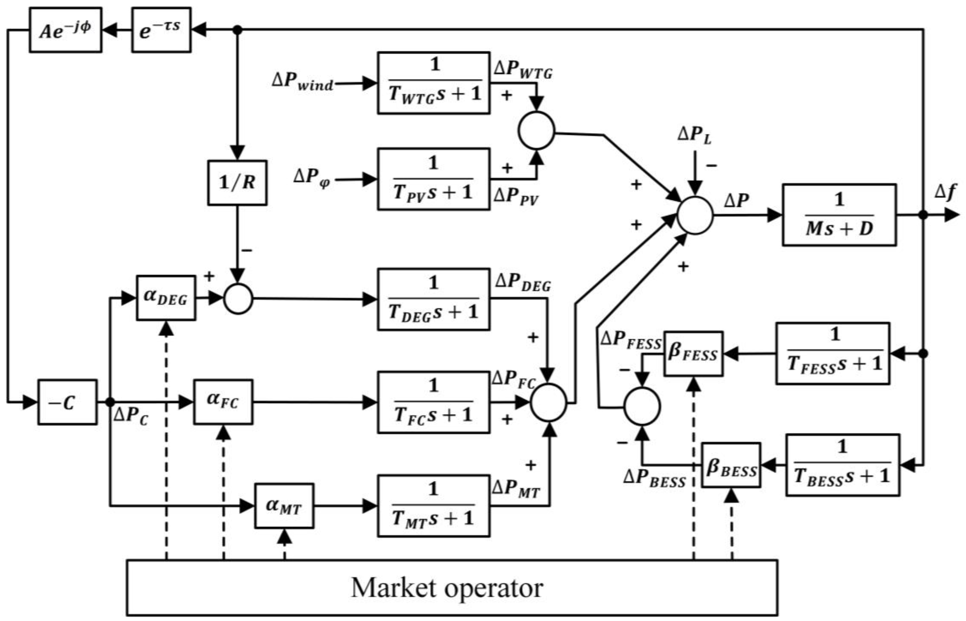
2. Mathematical Modeling of an MG System

In the configuration of the proposed method, several distributed energy resources (DER) are considered, including a flywheel energy storage system (FESS), a battery energy storage system (BESS), a fuel cell (FC) [25], a diesel engine generator (DEG) [26], a micro turbine (MT) [8], photovoltaic (PV) panels, and a wind turbine generator (WTG).

A review of the hierarchical control structure for MGs has been given in Section 1. It shows that, in the existing methods for the LFC issues of MGs, two level control (primary and secondary) has been widely investigated. However, the introduction of higher-level control (tertiary) into the MG model has received little attention. In this work, the well-known MG model proposed by [4] is considered. First, communication delay is introduced into this model. Then, for tertiary control, the participation factors of distributed energy resources are also introduced. With this, we expect the flexible configuration of the MG system. We also expect that the references of secondary control can be updated dynamically according to the actual application scenario. Note that the concept of participation factors is borrowed from the mature theory of conventional power systems [27]. The introduction of participation factors can realize the dynamic configuration and enhanced coordination of DER in the MG system.

The diagram of the MG system is shown in Figure 1. In this diagram, $\tau$ is communication delay, $\mathsf{\Delta }{P}_C$ is the supplementary control action, $A{e}^{-j\varphi }$ is the gain-phase margin tester that is nonexistent in the practical system [15], and $\mathsf{\Delta }{P}_{wind}$ and $\mathsf{\Delta }{P}_{\phi }$ are the Laplace transformations of wind speed and solar radiation, respectively. In this figure, ${\alpha }_{FC}$, ${\alpha }_{DEG}$, ${\alpha }_{MT}$, ${\beta }_{FESS}$, and ${\beta }_{BESS}$ are the participation factors of FC, DEG, MT, FESS, and BESS, respectively. These participation factors are scheduled by market operator (MO) [2,27,28] to make the most cost-effective combination of DER to meet their economic dispatch. Normally, in addition to non-negativity, these participation factors should satisfy:

$${\alpha }_{FC}+{\alpha }_{DEG}+{\alpha }_{MT}+{\beta }_{BESS}+{\beta }_{FESS}=1.$$

(1)

Energy storage systems play a fundamental role in achieving rapid frequency regulation by absorbing or injecting instantaneous power into MGs. Typical energy storage systems include FESS and BESS, which store reserved power in the form of kinetic and chemical energy, respectively. The transfer functions of FESS and BESS for active power control are given as [9,13].

$$G_{FESS}=\frac{K_{FESS}}{T_{FESS}s+1},G_{BESS}=\frac{K_{BESS}}{T_{BESS}s+1}.$$

(2)

It deserves noting that FESS and BESS are mainly used for transient power compensation via primary frequency control. After large frequency deviations are eliminated, the power output of energy storage systems should be restored to improve their service life and ensure the maximum emergency reserved power. In this case, distributed generators such as FC, DEG, and MT take over the power balancing task by participating in secondary frequency control. The transfer functions of FC, DEG, and MT are given as [9,19]

$$G_{FC}=\frac{K_{FC}}{T_{FC}s+1},G_{DEG}=\frac{K_{EDG}}{T_{DEG}s+1},G_{MT}=\frac{K_{MT}}{T_{MT}s+1}.$$

(3)

The larger the scale of RESs, the more predictable their power output will be. Compared with traditional large-scale power systems, the installed capacity of RESs in MGs is much smaller. This implies that it becomes more difficult to predict the power output of RESs in MGs. Hence, $\mathsf{\Delta }{P}_{WTG}$ and $\mathsf{\Delta }{P}_{PV}$ are considered disturbance signals [4,26] in this case study. The transfer functions of WTG and PV are given as [19]

$$G_{WTG}=\frac{1}{T_{WTG}s+1},G_{PV}=\frac{1}{T_{PV}s+1}.$$

(4)

The net power difference to evaluate the generation and demand balance can be expressed as

$$\begin{gathered} ∆P=\left({\alpha }_{FC}{G}_{FC}+{\alpha }_{DEG}{G}_{DEG}+{\alpha }_{MT}{G}_{MT}\right){∆P}_C \\ -\left(\frac{1}{R}{G}_{DEG}+{\beta }_{FESS}{G}_{FESS}{+\beta }_{BESS}{G}_{BESS}\right)∆f \\ +∆P_V+∆P_{WTG}-∆P_L. \end{gathered}$$

(5)

As can be seen from Figure 1 and Equation (5), DEG can be utilized to coordinate with FESS and BESS for transient power compensation support by adjusting its droop coefficient $R$.

The model parameters of the MG system in Figure 1 are shown in

Table 1. Model parameters of the MG system in Figure 1.

Parameter	Value	Parameter	Value
$M$	0.2	${K_{FESS},T}_{FESS}$	1, 0.1
$D$	0.012	${K_{BESS},T}_{BESS}$	1, 0.1
${K_{FC},T}_{FC}$	1, 4	$T_{WTG}$	1.5
${K_{DEG},T}_{DEG}$	1, 2	$T_{PV}$	1.8
${K_{MT},T}_{MT}$	1, 2	$R$	1.2

[4].

The objective of this work is to design a load frequency controller in the MG system to minimize the net power difference $\mathsf{\Delta }P$ under variations in participation factors, communication delay, and system model parameters.

3. Load Frequency Controller Design and Tuning

3.1. Load Frequency Controller Design

The stability boundary locus (SBL) method [15,23] is utilized for controller design. With the SBL method, the stable controller parameter space of the MG system can be determined. The load frequency controller parameters are obtained within the stability region to achieve the desired robustness and frequency regulation performance.

The adopted structure of the fractional-order load frequency controller is

$$C=K_P+K_I\frac{1}{s^{\lambda }}, 0<\lambda <2.$$

(6)

Denote $\theta =\left[K_P,K_I,\lambda \right]$. From Figure 1, we can obtain the characteristic equation of the closed-loop system as follows:

$$\begin{array}{l}\mathsf{\Delta }\left(\tau ,\theta ,A,\varphi ;s\right)\\ =P\left(s\right)+CQ\left(s\right)e^{-(\tau s+j\varphi )}\\ =\sum _{i=0}^6\left(p_i{s}^i\right)+C\sum _{\nu =0}^4\left(q_{\nu }{s}^{\nu }\right)e^{-(\tau s+j\varphi )}=0\end{array}$$

(7)

where

$$\begin{array}{ll}\hfill P\left(s\right)& =\left(T_{FC}s+1\right)\left(T_{MT}s+1\right)[\left(Ms+D\right)\\ & \left(T_{FESS}s+1\right)\left(T_{BESS}s+1\right)\left(T_{DEG}s+1\right)\\ & +{\beta }_{FESS}\left(T_{BESS}s+1\right)\left(T_{DEG}s+1\right)\\ & +{\beta }_{BESS}\left(T_{FESS}s+1\right)\left(T_{DEG}s+1\right)\\ & +1/R\left(T_{FESS}s+1\right)\left(T_{BESS}s+1\right)]\end{array}$$

$$\begin{array}{ll}\hfill Q\left(s\right)& =A\left(T_{FESS}s+1\right)\left(T_{BESS}s+1\right)\hfill \\ & [{\alpha }_{MT}\left(T_{FC}s+1\right)\left(T_{DEG}s+1\right)\\ & +{\alpha }_{DEG}\left(T_{FC}s+1\right)\left(T_{MT}s+1\right)\\ & +{\alpha }_{FC}\left(T_{DEG}s+1\right)\left(T_{MT}s+1\right)].\end{array}$$

The expressions $p_i$ and $q_{\nu }$ in (7) can be easily obtained from $P\left(s\right)$ and $Q\left(s\right)$, respectively. These expressions are somewhat lengthy and are not shown here to save space.

For the MG system under study, the boundaries of the stable controller parameters region can be determined by the complex root boundary (CRB) and real root boundary (RRB) as follows:

• RRB. The real root boundary is determined by $\mathsf{\Delta }\left(\tau ,\theta ,A,\varphi ;s=0\right)=0$, which, from (7), gives $K_I=0.$
• CRB. The complex root boundary is obtained by $\mathsf{\Delta }\left(\tau ,\theta ,A,\varphi ;s=j\omega \right)=$0. Inserting $s=j\omega$ and ${C|}_{s=j\omega }$ into (7), one obtains

$$\begin{array}{l}\mathsf{\Delta }\left(\tau ,\theta ,A,\varphi ;j\omega \right)\\ =y_1+j{y}_2+\left(K_P+K_I{\omega }^{-\lambda }\right)\left(y_3+j{y}_4\right)\\ \left[\mathrm{c}\mathrm{o}\mathrm{s}(\tau \omega +\varphi )-j\mathrm{s}\mathrm{i}\mathrm{n}(\tau \omega +\varphi )\right]=0\end{array}$$

(8)

where

$$y_1=-p_6{\omega }^6+p_4{\omega }^4-p_2{\omega }^2+p_0,$$

$$y_2=p_5{\omega }^5-p_3{\omega }^3+p_1\omega ,$$

$$y_3=q_4{\omega }^4-q_2{\omega }^2+q_0,$$

$$y_4=-q_3{\omega }^3+q_1\omega .$$

with $j^{-\lambda }=\mathrm{c}\mathrm{o}\mathrm{s}(\lambda \pi /2)-j\mathrm{s}\mathrm{i}\mathrm{n}(\lambda \pi /2)$, after some simple manipulation, the real and imaginary parts of (8) can be obtained respectively as follows:

$$\begin{array}{l}{K}_P\left[y_3\mathrm{c}\mathrm{o}\mathrm{s}(\tau \omega +\varphi )+y_4\mathrm{s}\mathrm{i}\mathrm{n}(\tau \omega +\varphi )\right]\\ {+K}_I{\omega }^{-\lambda }\left[y_3\mathrm{c}\mathrm{o}\mathrm{s}\right(\tau \omega +\varphi +\lambda \pi /2)\\ +y_4\mathrm{s}\mathrm{i}\mathrm{n}(\tau \omega +\varphi +\lambda \pi /2)]+y_1=0\end{array}$$

(9)

$$\begin{array}{l}{K}_P\left[y_4\mathrm{c}\mathrm{o}\mathrm{s}(\tau \omega +\varphi )-y_3\mathrm{s}\mathrm{i}\mathrm{n}(\tau \omega +\varphi )\right]\\ {+K}_I{\omega }^{-\lambda }\left[y_4\mathrm{c}\mathrm{o}\mathrm{s}\right(\tau \omega +\varphi +\lambda \pi /2)\\ -y_3\mathrm{s}\mathrm{i}\mathrm{n}(\tau \omega +\varphi +\lambda \pi /2)]+y_2=0\end{array}$$

(10)

From (9) and (10), one can obtain

$$K_P\left(\omega ,A,\varphi \right)=\frac{{ y}_1{ y}_6-{ y}_2{ y}_5-\mathrm{t}\mathrm{a}\mathrm{n}\left(\lambda \pi /2\right)({ y}_1{ y}_5+{ y}_2{ y}_6)}{{\omega }^{\lambda }\left(y_3^2+y_4^2\right)\mathrm{s}\mathrm{e}\mathrm{c}\left(\lambda \pi /2\right)}$$

(11)

$$K_I\left(\omega ,A,\varphi \right)=\frac{{ y}_2{ y}_5{-y}_1{ y}_6}{{\left(q_1\omega -q_3{\omega }^3\right)}^2{+\left(q_4{\omega }^4-q_2{\omega }^2+q_0\right)}^2}$$

(12)

where

$$y_5=y_3\mathrm{c}\mathrm{o}\mathrm{s}(\tau \omega +\varphi )+y_4\mathrm{s}\mathrm{i}\mathrm{n}(\tau \omega +\varphi )$$

$$y_6=y_4\mathrm{c}\mathrm{o}\mathrm{s}(\tau \omega +\varphi )-y_3\mathrm{s}\mathrm{i}\mathrm{n}(\tau \omega +\varphi ).$$

Hence, for a fixed $\lambda$, the CRB is determined by plotting the curve of $K_P$ versus $K_I$ with $\omega \to +\infty$ from zero. With $A=1,\varphi =0°$, and a given fractional order $\lambda$, the stable parameters plane $\left(K_P,K_I\right)$ can be obtained from the CRB and RRB curves presented above. The stability region can be determined by a random point testing method [29].

The controller gains $K_P$ and $K_I$ can be determined within the stability region or the relative stability region which satisfies specified GM and PM.

3.2. Tuning of Fractional Order

Phase margin (PM) is a common robustness index for FOPI controller tuning [23,24]. In this tuning method, the controller parameters $K_P$ and $K_I$ are obtained within the stable parameters plane $\left(K_P,K_I\right)$ satisfying the desired PM $\varphi$ and gain crossover frequency ${\omega }_{gc}$, which corresponds to the black circle “N” in Figure 2a. However, it is not clear whether this tuning method can achieve the desired gain margin (GM) of the closed-loop system. Another widely accepted SBL tuning method is the weighted geometrical center method [30], corresponding to point “P” in this figure. This method is simple and intuitive. The controller parameters are calculated based on the weighted geometric center of the stability region. Nevertheless, despite offering good performance, it remains uncertain whether this method can obtain the desired system robustness in terms of GM and PM.

To have design with guaranteed GM and PM, the controller parameters should be tuned within the shaded region in Figure 2a. In this work, the tuning parameters $K_P$ and $K_I$ are chosen as the intersection “M” of the relative stability curves in this region. The reason for this choice is that ${\omega }_{gc}$ at this intersection is the maximum gain crossover frequency that can be achieved within the shaded region. This implies that better frequency regulation performance can be obtained, since a larger value of ${\omega }_{gc}$ usually gives a faster response speed [24].

The flat phase constraint (FPC) ensures a smooth open-loop phase at the gain crossover frequency, which enhances system robustness with respect to loop gain variations. Therefore, this constraint is utilized to cope with the frequency stability issue caused by gain perturbations in $K_{FC}$, $K_{DEG}$, and $K_{MT}$ in the studied MG system. To have a unique load frequency controller tuning, the fractional order $\lambda$ is calculated to satisfy this constraint [23,24]:

$$\frac{\mathrm{d}\varphi }{\mathrm{d}\omega }=0,0<\lambda <2.$$

(13)

In order to obtain the expression of $\varphi$, once again we divide $\mathsf{\Delta }\left(\tau ,\theta ,A,\varphi ;s=j\omega \right)$ into real and imaginary part equations, as follows:

$$\begin{gathered} y_1+\left(r_1{y}_3-r_2{y}_4\right)\cos \left(\tau \omega +\varphi \right) \\ +(r_1{y}_4+r_2{y}_3)\mathrm{s}\mathrm{i}\mathrm{n}(\tau \omega +\varphi )=0 \end{gathered}$$

(14)

$$\begin{gathered} y_2+\left(r_1{y}_4+r_2{y}_3\right)\cos \left(\tau \omega +\varphi \right) \\ -(r_1{y}_3-r_2{y}_4)\mathrm{s}\mathrm{i}\mathrm{n}(\tau \omega +\varphi )=0 \end{gathered}$$

(15)

From (14) and (15), we get

$$\varphi =\mathrm{a}\mathrm{r}\mathrm{c}\mathrm{t}\mathrm{a}\mathrm{n}\frac{x_2{y}_1-x_1{y}_2}{x_1{y}_1+x_2{y}_2}-\tau \omega +n\pi$$

(16)

where

$$x_1{=r}_1{y}_3-r_2{y}_4$$

$$x_2=r_1{y}_4+r_2{y}_3$$

$$r_1=K_P+K_I{\omega }^{-\lambda }\mathrm{c}\mathrm{o}\mathrm{s}\left(\lambda \pi /2\right)$$

$$r_2=-K_I{\omega }^{-\lambda }\mathrm{s}\mathrm{i}\mathrm{n}\left(\lambda \pi /2\right).$$

Substituting (16) into (13) gives

$$\frac{\mathrm{d}\varphi }{\mathrm{d}\omega }=\frac{x_1\acute{x_2}-\acute{x_1}{x}_2}{x_1^2+x_2^2}+\frac{\acute{y_1}{y}_2-y_1\acute{{\mathrm{y}}_2}}{y_1^2+y_2^2}-\tau =0$$

(17)

where

$$\acute{y_1}=-6p_6{\omega }^5+4p_4{\omega }^3-2p_2\omega$$

$$\acute{y_2}=5p_5{\omega }^4-3p_3{\omega }^2+p_1$$

$$\acute{x_1}=\acute{r_1}{y}_3+r_1\acute{y_3}-\acute{r_2}{y}_4-r_2\acute{y_4}$$

$$\acute{x_2}=\acute{r_1}{y}_4+r_1\acute{y_4}+\acute{r_2}{y}_3+r_2\acute{y_3}$$

$$\acute{y_3}=4q_4{\omega }^3-2q_2\omega$$

$$\acute{y_4}=-3q_3{\omega }^2+q_1$$

$$\acute{r_1}=-\lambda K_I{\omega }^{-\lambda -1}\mathrm{c}\mathrm{o}\mathrm{s}\left(\lambda \pi /2\right)$$

$$\acute{r_2}=\lambda K_I{\omega }^{-\lambda -1}\mathrm{s}\mathrm{i}\mathrm{n}\left(\lambda \pi /2\right).$$

3.3. Design Summary and Tuning Algorithm

The design summary with an MG example is given as follows:

Step 1. The MG model parameters are shown in Table 1. Fix participation factors as: ${\alpha }_{MT}=0.1,{\alpha }_{DEG}=0.17,{\alpha }_{FC}=0.23$, ${\beta }_{BESS}=0.15$, ${\beta }_{FESS}=0.35$. The fractional order is also fixed at first. (For illustration, it is taken as $\lambda =1.1$ in this example.) Given $A=1$ and $\varphi =0°$, the CRB curve of $K_P$ versus $K_I$ is plotted according to (11) and (12). The RRB line is determined as $K_I=0$. The stability region circled by CRB and RRB is shown in Figure 2a, which can be determined by testing a random point in each divided region.

Step 2. Select the desired GM and PM values, such as $A=3$ and $\varphi =60°$. With (11) and (12), the relative stability line (RSL) of GM and PM is obtained as the dash-dotted line and the dashed line in Figure 2a, respectively, through which the parameters $K_P$ and $K_I$ at intersection M can be read.

Step 3. Test whether the flat phase constraint (FPC) is satisfied by substituting the obtained controller parameters ($K_P$, $K_I$, and $\lambda$) into (17). If it is satisfied, stop the algorithm. Otherwise, sweep the fractional order in the range $\lambda \in \left(\mathrm{0,2}\right)$, as shown in Figure 2b, until the flat phase point (FPP) which satisfies the desired GM, PM, and FPC is found.

For clear presentation, the SBL GM curves of $A=3$ and $\varphi =0°$ are not shown in Figure 2b.

The flow chart of the above design steps is depicted in Figure 3a.

It is worth noting that the controller parameters of the proposed method are obtained in a similar way to the recent ref. [24], although the achieved system robustness is quite different. For both methods, one common disadvantage is that only crude controller parameters can be obtained, if the tuning is conducted as per the design steps mentioned above. Because the interval of fractional order $\lambda$ cannot be taken too small, otherwise the tuning process will be rather time-consuming. To face this issue, an automatic algorithm for calculating intersection coordinates is developed in this work, which can greatly reduce the tuning burden.

It should be stressed that the SBL curves with specified GM and PM are both parametric equation curves. Therefore, the controller parameters of the proposed method can be tuned through an algorithm searching the intersection of these two parametric equation curves, according to Equations (11) and (12). To conduct this searching algorithm, the SBL curve with specified GM is denoted as $C_1$ with $K_{P1}=f({\omega }_{180},A,\varphi =0°)$ and $K_{I1}=f({\omega }_{180},A,\varphi =0°)$, where ${\omega }_{180}$ is the phase crossover frequency. On the other hand, the SBL line with specified PM is expressed as $C_2$ with $K_{P2}=f({\omega }_{gc},A=1,\varphi )$ and $K_{I2}=f({\omega }_{gc},A=1,\varphi )$. Given initial frequency guess values of ${\omega }_{gc}$ and ${\omega }_{180}$, the intersection can be easily computed by MATLAB function fminsearch for a fixed fractional order $\lambda$. Then, scanning the fractional order and using MATLAB function min to find the minimal value $\left|\mathrm{d}\varphi /\mathrm{d}\omega \right|$, the tuning parameters at FPP can be found. Note from Figure 2a that two intersection points may exist, and inappropriate tuning can be avoided by selecting reasonable initial frequency guess values (not too small).

The proposed tuning algorithm to obtain controller tuning parameters is shown in Figure 3b.

4. Tuning Analysis under Perturbed Model Parameters

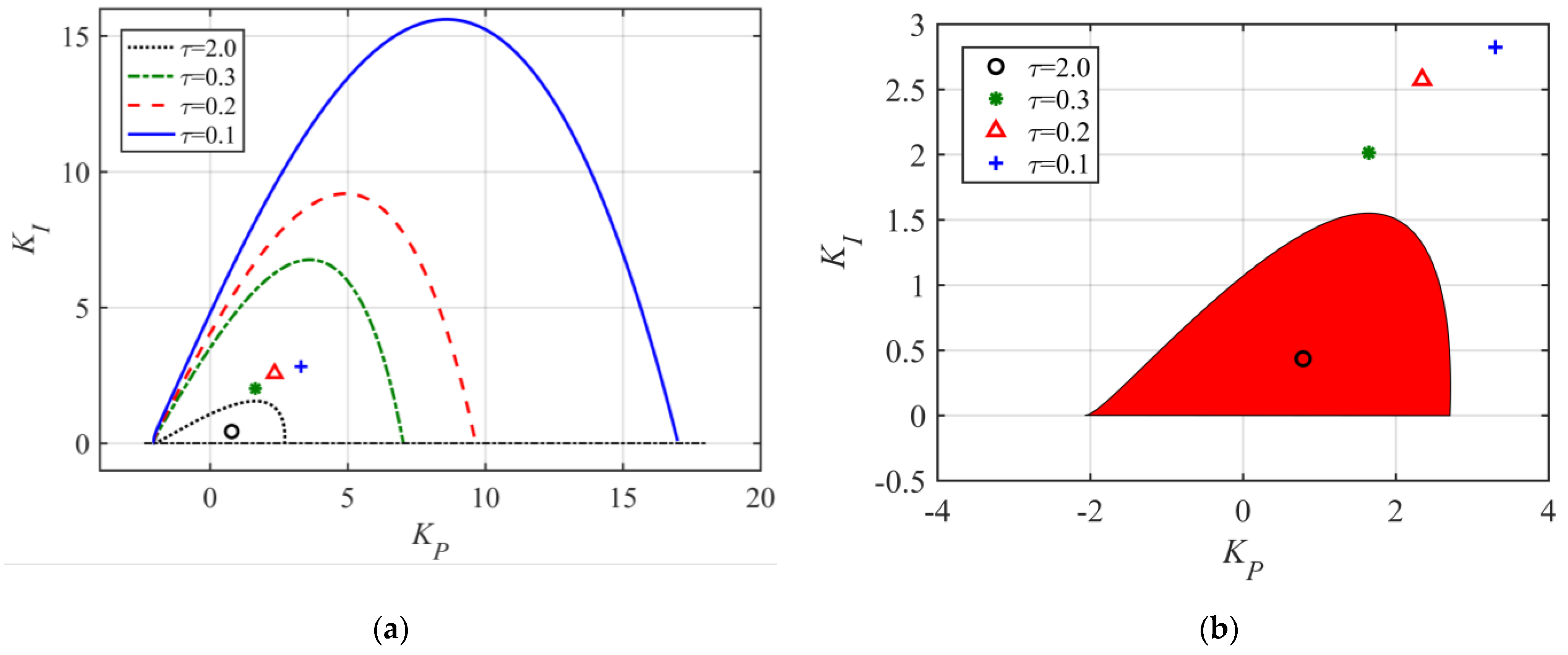
4.1. Controller Tuning under Perturbed Communication Delay

In practical engineering applications, communication delay can hardly be precisely estimated in the MG system. Usually, only a perturbation interval of communication delay can be determined. Therefore, it is meaningful to have controller tuning based on a common stability region for all possible variations in communication delay.

To investigate the influence of communication delay on controller tuning, the fractional order and participation factors are fixed as $\lambda =1.1$ and ${\alpha }_{MT}=0.2,{\alpha }_{DEG}=0.2,{\alpha }_{FC}=0.2$, ${\beta }_{BESS}=0.2$, ${\beta }_{FESS}=0.2$, respectively. The stability regions ($A=1$ and $\varphi =0°$) under different communication delays are shown in Figure 4a. The tuning parameters satisfying the desired GM and PM of $A=3$ and $\varphi =60°$ are also shown in this figure, as marked with symbols with the color kept the same in each case. For $\tau =0.1$, the tuning parameters by $A=3$ and $\varphi =60°$ do not exist according to the proposed tuning algorithm, so, in this case, $A=4$ and $\varphi =60°$ are chosen as robustness indices. The common stability region is shown in Figure 4b.

It is shown that the variation in communication delay has a dramatic impact on system stability. As $\tau$ increases, the size of the stability region shrinks significantly. This gives an important insight for designing a load frequency controller with uncertain communication delay. Since the stability region for a larger communication delay is a subset of the region for a smaller one, it is safer to have an upper bound estimation of $\tau$ to design the load frequency controller. In this way, system stability can be guaranteed for all possible perturbations of communication delay.

4.2. Controller Tuning under Perturbed Model Gains

Assume that ${\alpha }_{MT}=0.2,{\alpha }_{DEG}=0.2,{\alpha }_{FC}=0.2$, ${\beta }_{BESS}=0.2$, ${\beta }_{FESS}=0.2.$ In this Section, the frequency regulation performance is compared between PI and FOPI control, under perturbed MG model gains. With $A=3$, $\varphi =60°$, and FPC, the controller parameters are obtained as $K_P=0.9411$, $K_I=0.2773$, and $\lambda =1.2301$ for the POPI controller, according to the proposed tuning algorithm in Section 3.3. With the same values of $A$ and $\varphi$, the parameters obtained are $K_P=0.5108$ and $K_I=0.5192$ for PI controller.

Assume that MG model gains change within $K_{MT}\in \left[\mathrm{0.8,1.2}\right]$, $K_{DEG}\in \left[\mathrm{0.8,1.2}\right]$, and $K_{FC}\in \left[\mathrm{0.8,1.2}\right]$. Load disturbance of ${∆P}_L=0.1$ p.u. is applied, under these gain perturbations. The frequency response results are shown in Figure 5. It is shown that, under the action of the load frequency controller, the change happens at the second wave peak of the frequency response. FOPI control, which yields a maximum peak value of 0.0128, has stronger loop robustness than PI control, which gives a maximum peak value of 0.0218. The designed PI controller cannot satisfy the FPC index well due to the lack of an additional degree of freedom.

Note that the proposed method is scalable and adaptable to different microgrid systems with varying communication delays and uncertain model gains by adjusting the participation factors of the system model. With the introduction of different participation factors, the power reference values of different micro sources can be given. The variation of participation factors corresponds to different microgrid systems with varying communication delays and uncertain model gains.

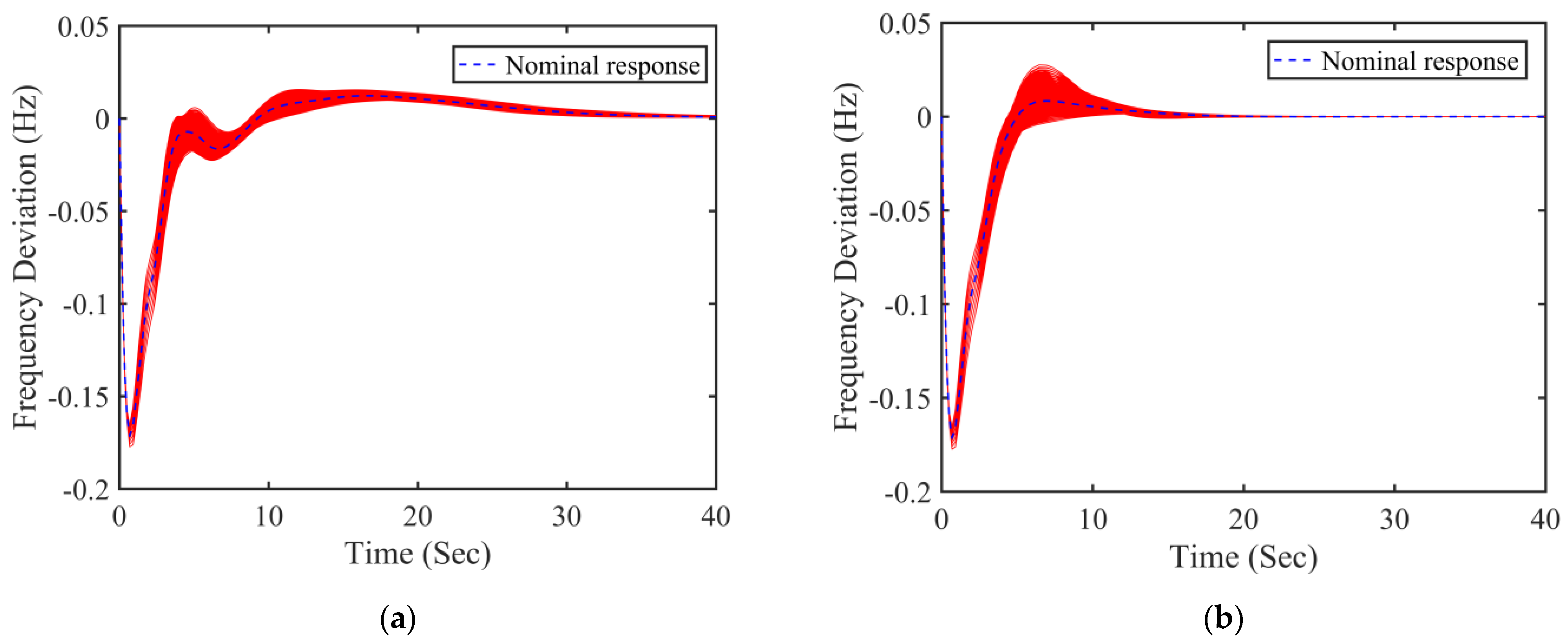
5. Simulation Results

The proposed FOPI tuning method is compared with classical FOPI methods [23,24] in Section 5.1. In Section 5.2, the frequency response results are shown under the influence of participation factors and droop coefficient of DEG, respectively. In Section 5.3, the simulation results are shown under uncertain communication delay.

Both load disturbance and real-world solar radiation and wind power fluctuation data are utilized to evaluate the effectiveness of the proposed tuning method. The solar radiation data used are from Aberdeen (United Kingdom) [10], while the wind power fluctuation data are taken from the National Renewable Energy Laboratory (NREL) [31]. The power fluctuations of PV and WTG are depicted in Figure 6.

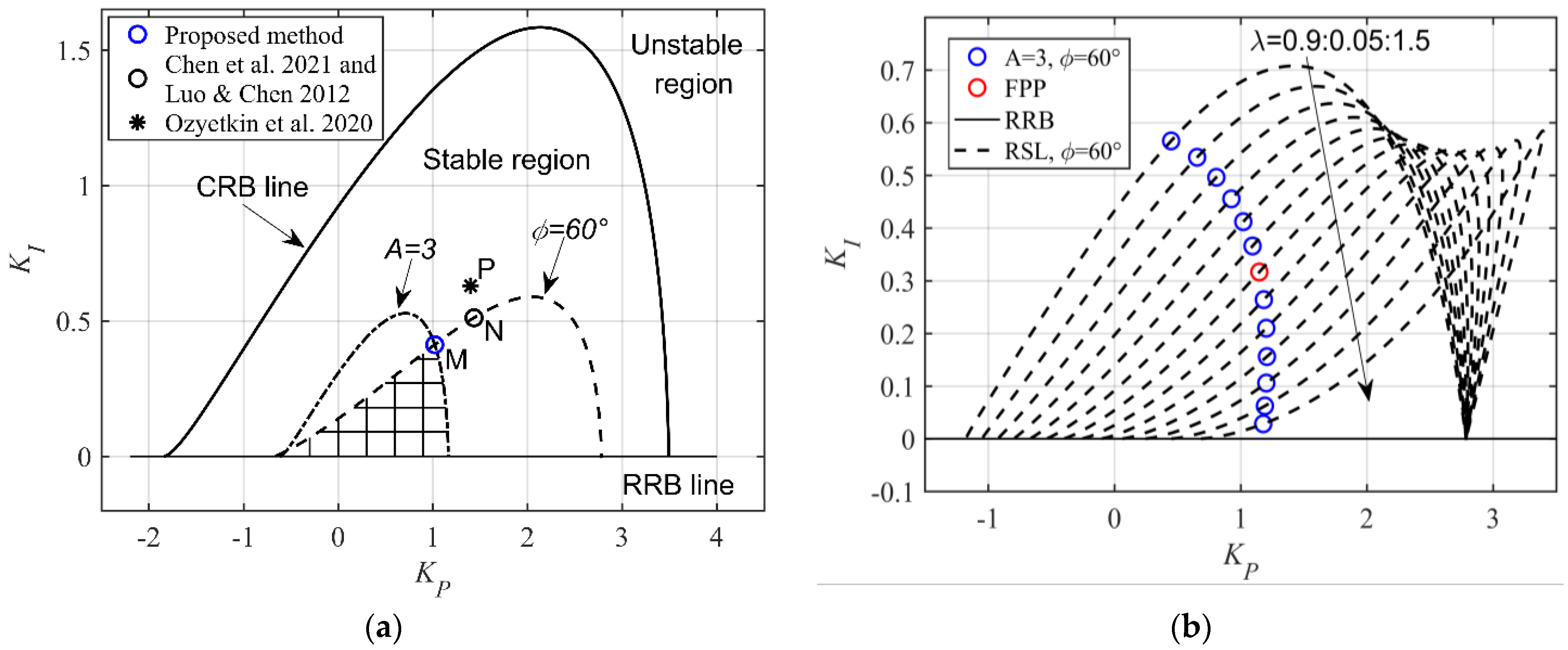
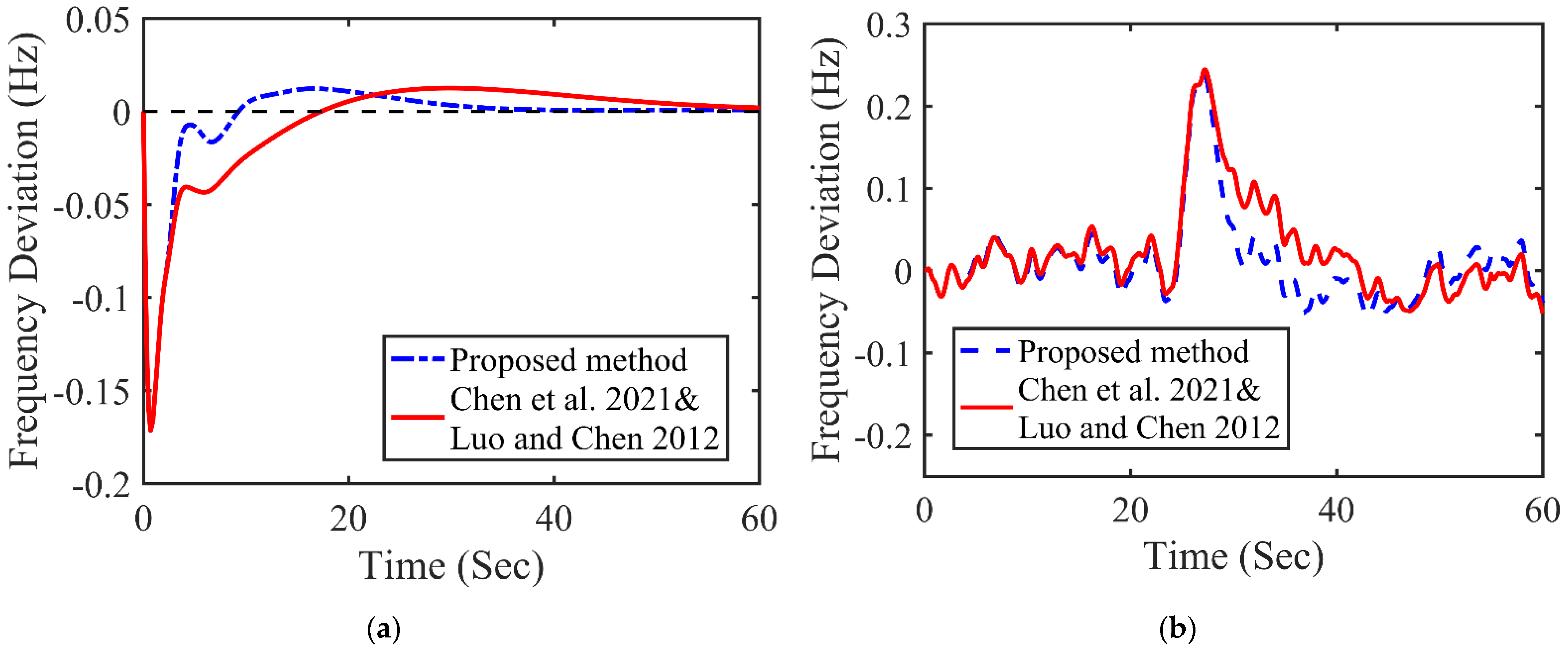
5.1. Comparison with Classical FOPI Tuning Method

Assume that ${\alpha }_{MT}=0.2,{\alpha }_{DEG}=0.2,{\alpha }_{FC}=0.2$, ${\beta }_{BESS}=0.2$, ${\beta }_{FESS}=0.2.$ With $A=3$, $\varphi =60°$, and FPC, the controller parameters are obtained as $K_P=0.9411$, $K_I=0.2773$, and $\lambda =1.2301$ for the proposed POPI controller tuning. Selecting ${\omega }_{gc}=0.1,\varphi =60°$, and FPC, the controller parameters are obtained as $K_P=0.5491$, $K_I=0.1228$, and $\lambda =1.27$ for the methods in [23,24]. The simulation results under a load disturbance of ${∆P}_L=0.1$ and under wind and solar power injection are shown in Figure 7a,b, respectively.

The impact of the load frequency controller happens at the second wave peak of the frequency response. It is shown that the proposed method gives a significantly faster response speed than the classical methods in [23,24]. On the other hand, as shown in Figure 7b, the maximum frequency deviation exceeds 0.2 Hz, which may trigger some safety limitations. In this case, energy storage systems such as FESS and BESS should take more responsibility by increasing their participation factors to speed up the frequency response.

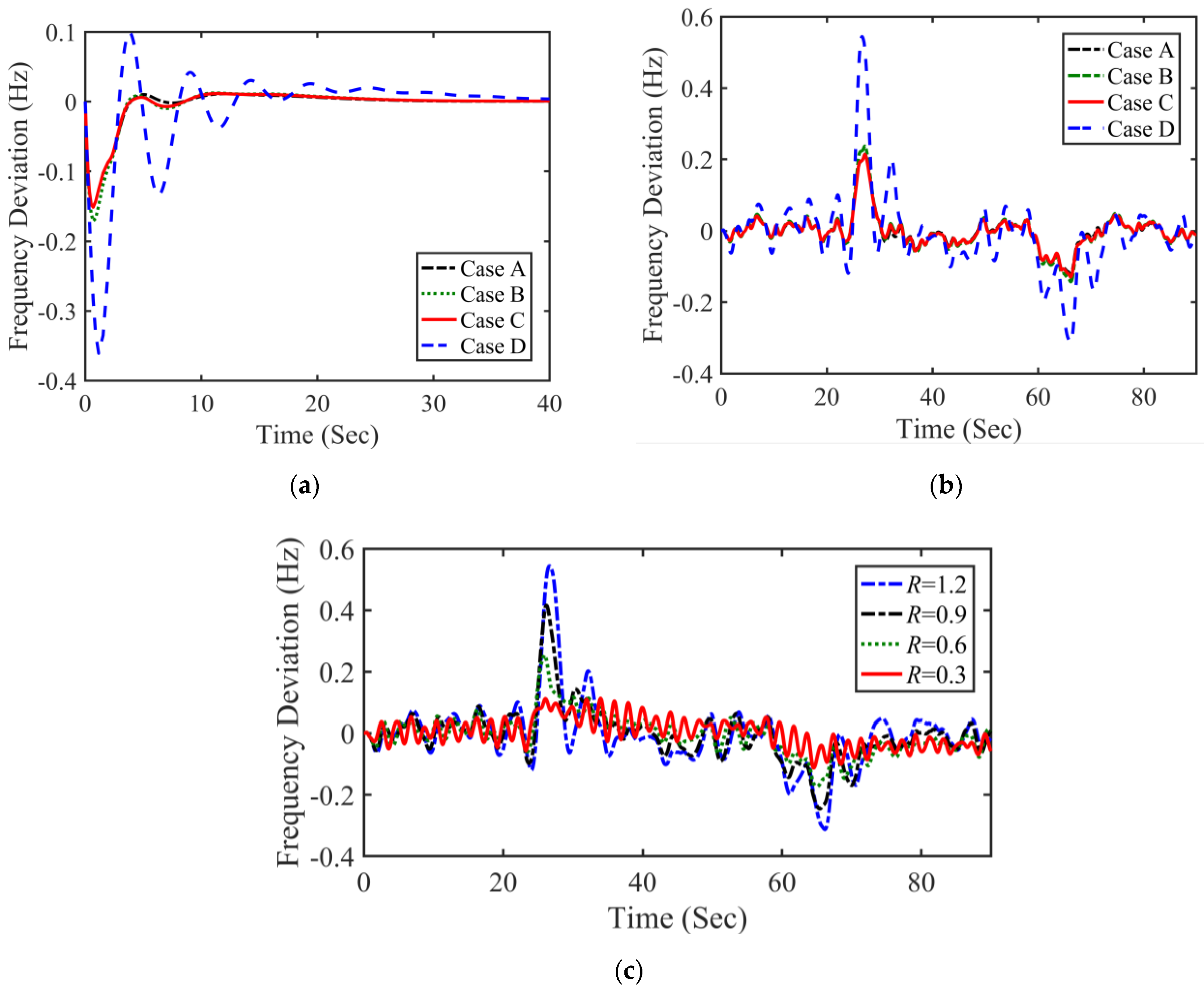
5.2. Influence of Participation Factors

The MG model parameters are shown in Table 1. The communication delay is fixed as $\tau =2$. To investigate the influence of participation factors on frequency regulation performance, the following four cases of DER combinations are considered:

(1)

Case A. Only FC participates in secondary frequency control: ${\alpha }_{MT}=0,{\alpha }_{DEG}=0,{\alpha }_{FC}=0.5$, ${\beta }_{BESS}=0.25$, ${\beta }_{FESS}=0.25$;

(2)

Case B. Uniform coordination of different DER: ${\alpha }_{MT}=0.2,{\alpha }_{DEG}=0.2,{\alpha }_{FC}=0.2$, ${\beta }_{BESS}=0.2$, ${\beta }_{FESS}=0.2$;

(3)

Case C. Both MT and DEG participate in secondary frequency control: ${\alpha }_{MT}=0.25,{\alpha }_{DEG}=0.25,{\alpha }_{FC}=0$, ${\beta }_{BESS}=0.25$, ${\beta }_{FESS}=0.25$;

(4)

Case D. Only FC participates in secondary frequency control and both BESS and FESS are switched off: ${\alpha }_{MT}=0,{\alpha }_{DEG}=0,{\alpha }_{FC}=1$, ${\beta }_{BESS}=0$, ${\beta }_{FESS}=0$.

With $A=2.5,\varphi =60°$, and FPC, the controller parameters are obtained as $K_P=2.347$, $K_I=0.5307$, and $\lambda =1.196$ for case A, $K_P=1.123$, $K_I=0.3475$, and $\lambda =1.220$ for case B, $K_P=1.342$, $K_I=0.4263$, and $\lambda =1.246$ for case C, and $K_P=0.3551$, $K_I=0.0846$, and $\lambda =1.226$ for case D, respectively. The frequency response results for these cases in the presence of load disturbance ${∆P}_L=0.1$ and the output power fluctuations of PV and WTG are shown in Figure 8a,b, respectively.

It is observed from Figure 8a that, for cases A, B, and C, superior frequency regulation performance can be obtained. The maximum frequency deviations are within $\pm$0.2 Hz, which can meet the standard of frequency limit for distribution grid in China. However, in Case D, the maximum frequency deviation exceeds 0.2 Hz. The excess of deviation might be unacceptable in some applications, and it is challenging to substantially improve the frequency response just through an advanced control method. The reason for this is that both FESS and BESS are switched off in this case, implying that there are not enough fast power regulation devices to participate in primary frequency control. A large transient power deficit cannot be effectively compensated by secondary frequency control, which is relatively sluggish, especially in the presence of a substantial communication delay.

The above analysis shows that FESS and BESS are important components for the MG system to achieve the rapid regulation of the frequency response. When these components are insufficient to provide transient power compensation, some other DER should participate in primary frequency control. To improve frequency regulation performance of case D, DEG takes over the functions of FESS and BESS, by adjusting the droop coefficient $R$ for primary frequency regulation. With controller parameters fixed as $K_P=0.3551$, $K_I=0.0846$, and $\lambda =1.226$, the frequency response results under the variation of droop coefficient are shown in Figure 8c. It can be concluded that the performance can be significantly improved by gradually reducing the droop coefficient.

Note that fixed controller parameters have been utilized to investigate the influence of the droop coefficient. Hence, even better performance can be obtained if the variation of $R$ is incorporated into controller design as per the proposed tuning algorithm in Section 3.3. On the other hand, future study is needed to unearth the compensation limitations and potential of DEG in order to determine the feasible range of $R$ for application in practical engineering.

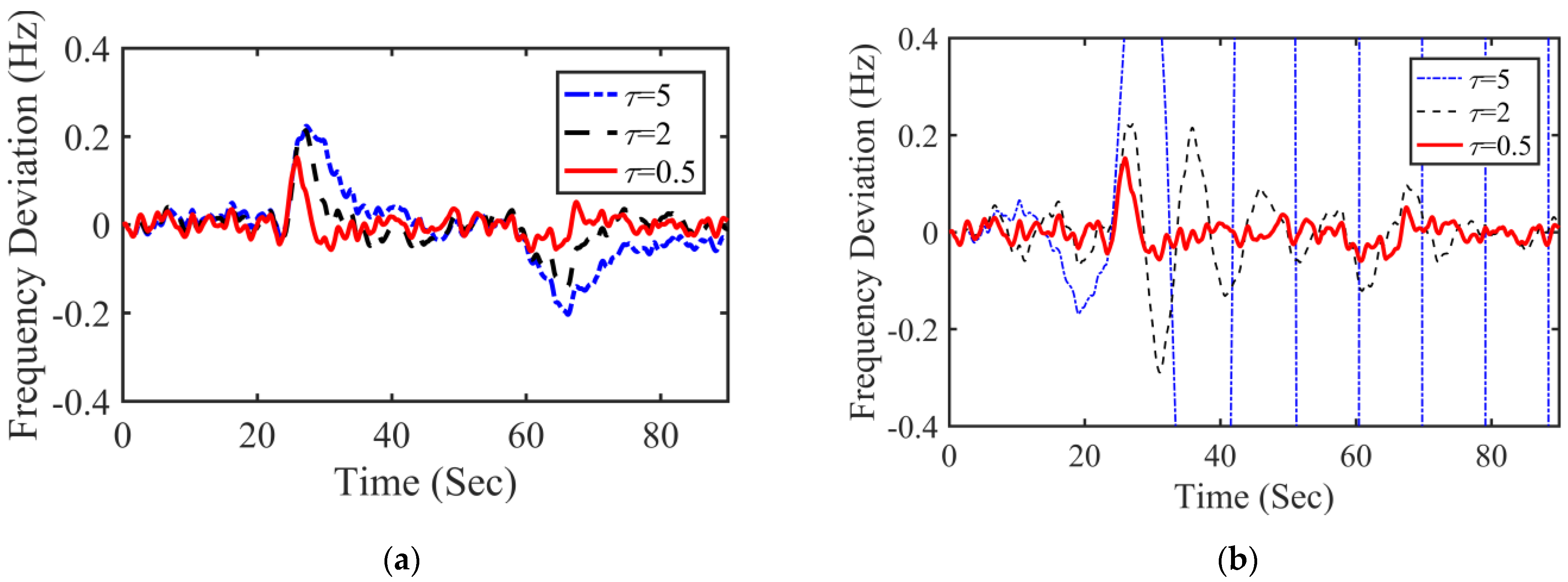
5.3. Influence of Communication Delay

The communication delay of the MG system can hardly be precisely estimated. Since significant estimation error may exist, it is meaningful to evaluate the influence of communication delay on system stability and frequency regulation performance. In reality, only the approximate range (such as $\tau \in \left[0.5, 5\right]$ considered in this Section) of communication delay can be determined. In this range, we consider three typical delay values for illustration purposes, i.e., $\tau =0.5$, $2$, and $5$. Participation factors are fixed as ${\alpha }_{MT}=0.1,{\alpha }_{DEG}=0.17,{\alpha }_{FC}=0.23$, ${\beta }_{BESS}=0.15$, ${\beta }_{FESS}=0.35$. With $A=3, \varphi =60°$, and FPC, the tuning parameters of the proposed FOPI controller are obtained as $K_P=2.328$, $K_I=1.828$, and $\lambda =1.191$ for $\tau =0.5$, $K_P=1.395$, $K_I=0.392$, and $\lambda =1.218$ for $\tau =2$, and $K_P=1.204$, $K_I=0.1335$, and $\lambda =1.245$ for $\tau =5$, respectively. Here, we refer to the above settings as exact tuning, because the desired system robustness can be achieved for each exact value of $\tau$.

The corresponding frequency response results under PV and WTG power fluctuations are shown in Figure 9a. It is observed that frequency regulation performance gradually improves as communication delay decreases. On the other hand, the maximum frequency deviations are within $\pm$0.2 Hz for $\tau =0.5$, which can meet the standard of frequency limit for the distribution grid in China.

It is interesting to see that the analysis in Figure 9a is based on the assumption that communication delay can be precisely estimated, with controller parameters updated to track the variation of $\tau$. Since precise estimation rarely happens in practice, a more common choice is to conduct design in terms of the estimated delay value. To evaluate the effect of this choice, the frequency responses with tuning based on estimation $\tau =0.5$ (aggressive tuning) and $\tau =5$ (conservative tuning) are shown in Figure 9b,c, respectively.

It can be concluded that, with aggressive tuning, the frequency response is unstable for $\tau =5$. While under conservative tuning, satisfactory regulation performance can be obtained for all values of communication delay, although with slight performance deterioration for $\tau =0.5$ and $2$. These conclusions are consistent with the analysis of the influence of communication delay, as presented in Section 4. Because the size of the stability region gradually shrinks as $\tau$ increases, a feasible tuning with acceptable performance should be conducted via an upper bound estimation of communication delay.

Note that more precious quantitative assessment could be provided by adding integral error performance indices (like IAE, ITAE, and ISE) to compare the proposed method with the classical tuning methods.

6. Conclusions

In this paper, a robust fractional-order PI (FOPI) tuning method is proposed for the LFC issue of a microgrid (MG) with communication delay. We have introduced participation factors in the MG system model to realize the flexible configuration and enhanced coordination of distributed energy resources to improve frequency response. The load frequency controller is designed based on this model to achieve the desired system robustness in terms of gain margin, phase margin, and the flat phase constraint. Compared with conventional PI control, the proposed FOPI method has significantly better system robustness with respect to model gain variations in FC, DEG, and MT. Comparison with the classical FOPI tuning method is also presented to show the effectiveness of the proposed tuning method.

With the proposed FOPI controller tuning, the frequency regulation performance is evaluated under the influence of participation factors and uncertain communication delay. The influence of participation factors shows that FESS and BESS play a critical role in obtaining rapid frequency regulation and active power compensation. The influence of communication delay shows that conservative tuning utilizing the upper bound delay estimation is a feasible way to design a load frequency controller with acceptable frequency response.

The limitation of the proposed method is that it is not as easy-to-use as tuning rules-based methods. Hence, future work aims at developing tuning rules for microgrid systems with communication delay based on the proposed stability boundary locus method.

References

1. Bevrani HFrancois, B.; Ise, T. Microgrid Dynamics and Control; John Wiley & Sons: Hoboken, NJ, USA, 2017. [Google Scholar]
2. Meng, L.; Sanseverino, E.R.; Luna, A.; Dragicevic, T.; Vasquez, J.C.; Guerrero, J.M. Microgrid supervisory controllers and energy management systems: A literature review. Renew. Sustain. Energy Rev. 2016, 60, 1263–1273. [Google Scholar] [CrossRef]
3. Jirdehi, M.A.; Tabar, V.S.; Ghassemzadeh, S.; Tohidi, S. Different aspects of microgrid management: A comprehensive review. J. Energy Storage 2020, 30, 101457. [Google Scholar] [CrossRef]
4. Bevrani, H.; Feizi, M.R.; Ataee, S. Robust frequency control in an islanded microgrid: H and μ-Synthesis Approaches. IEEE Trans. Smart Grid. 2016, 7, 706–717. [Google Scholar] [CrossRef] [Green Version]
5. Katiraei, F.; Iravani, R.; Hatziargyriou, N.; Dimeas, A. Microgrid management. IEEE Power Energy Mag. 2008, 6, 54–65. [Google Scholar] [CrossRef]
6. Bidram, A.; Davoudi, A. Hierarchical structure of microgrids control system. IEEE Trans. Smart Grid 2012, 3, 1963–1976. [Google Scholar] [CrossRef]
7. Jain, S.; Hote, Y.V. Generalized active disturbance rejection controller design: Application to hybrid microgrid with communication delay. Int. J. Electr. Power Energy Syst. 2021, 132, 107166. [Google Scholar] [CrossRef]
8. Yildirim, B.; Khooban, M.H. Enhancing stability region of time-delayed smart power grids by non-integer controllers. Int. J. Energy Res. 2021, 45, 541–553. [Google Scholar] [CrossRef]
9. Özdemir, M.T. The effects of the FOPI controller and time delay on stability region of the fuel cell microgrid. Int. J. Hydrogen Energy 2020, 45, 35064–35072. [Google Scholar] [CrossRef]
10. Khooban, M.-H.; Dragicevic, T.; Blaabjerg, F.; Delimar, M. Shipboard Microgrids: A Novel Approach to Load Frequency Control. IEEE Trans. Sustain. Energy 2018, 9, 843–852. [Google Scholar] [CrossRef]
11. Khooban, M.H.; Gheisarnejad, M. A Novel Deep Reinforcement Learning Controller Based Type-II Fuzzy System: Frequency Regulation in Microgrids. IEEE Trans. Emerg. Top. Comput. Intell. 2020, 5, 689–699. [Google Scholar] [CrossRef]
12. Khooban, M.H.; Niknam, T.; Blaabjerg, F.; Dragičević, T. A new load frequency control strategy for micro-grids with considering electrical vehicles. Electr. Power Syst. Res. 2017, 143, 585–598. [Google Scholar] [CrossRef] [Green Version]
13. Mandal, R.; Chatterjee, K. Frequency control and sensitivity analysis of an isolated microgrid incorporating fuel cell and diverse distributed energy sources. Int. J. Hydrogen Energy 2020, 45, 13009–13024. [Google Scholar] [CrossRef]
14. Khalil, A.; Rajab, Z.; Alfergani, A.; Mohamed, O. The impact of the time delay on the load frequency control system in microgrid with plug-in-electric vehicles. Sustain. Cities Soc. 2017, 35, 365–377. [Google Scholar] [CrossRef]
15. Yildirim, B. Advanced controller design based on gain and phase margin for microgrid containing PV/WTG/Fuel cell/Electrolyzer/BESS. Int. J. Hydrogen Energy 2021, 46, 16481–16493. [Google Scholar] [CrossRef]
16. Gu, W.; Liu, W.; Wu, Z.; Zhao, B.; Chen, W. Cooperative Control to Enhance the Frequency Stability of Islanded Microgrids with DFIG-SMES. Energies 2013, 6, 3951–3971. [Google Scholar] [CrossRef]
17. Yang, J.; Zeng, Z.; Tang, Y.; He, H.; Wu, Y. Load Frequency Control in Isolated Micro-Grids with Electrical Vehicles Based on Multivariable Generalized Predictive Theory. Energies 2015, 8, 2145–2164. [Google Scholar] [CrossRef]
18. Sahu, P.C.; Mishra, S.; Prusty, R.C.; Panda, S. Improved-salp swarm optimized type-II fuzzy controller in load frequency control of multi area islanded AC microgrid. Sustain. Energy Grids Netw. 2018, 16, 380–392. [Google Scholar] [CrossRef]
19. Khokhar, B.; Dahiya, S.; Parmar, K.S. Load frequency control of a microgrid employing a 2D Sine Logistic map based chaotic sine cosine algorithm. Appl. Soft Comput. 2021, 109, 107564. [Google Scholar] [CrossRef]
20. Latif, A.; Chandra Das, D.; Kumar Barik, A.; Ranjan, S. Illustration of demand response supported co-ordinated system performance evaluation of YSGA optimized dual stage PIFOD-(1+PI) controller employed with wind-tidal-biodiesel based independent two-area interconnected microgrid system. IET Renew. Power Gener. 2020, 14, 1074–1086. [Google Scholar] [CrossRef]
21. Bošković, M.; Šekara, T.B.; Rapaić, M.R. Novel tuning rules for PIDC and PID load frequency controllers considering robustness and sensitivity to measurement noise. Int. J. Electr. Power Energy Syst. 2020, 114, 105416. [Google Scholar] [CrossRef]
22. Sun, L.; Xue, W.; Li, D.; Zhu, H.; Su, Z.G. Quantitative tuning of active disturbance rejection controller for FOPDT model with application to power plant control. IEEE Trans. Ind. Electron. 2022, 69, 805–815. [Google Scholar] [CrossRef]
23. Luo, Y.; Chen, Y.Q. Stabilizing and robust fractional order PI controller synthesis for first order plus time delay systems. Automatica 2012, 48, 2159–2167. [Google Scholar] [CrossRef]
24. Chen, P.; Luo, Y.; Peng, Y.; Chen, Y. Optimal robust fractional order PIλD controller synthesis for first order plus time delay systems. ISA Trans. 2021, 114, 136–149. [Google Scholar] [CrossRef] [PubMed]
25. Sun, L.; Wu, G.; Xue, Y.; Shen, J.; Li, D.; Lee, K.Y. Coordinated Control Strategies for Fuel Cell Power Plant in a Microgrid. IEEE Trans. Energy Convers. 2018, 33, 1–9. [Google Scholar] [CrossRef]
26. Rafiee, A.; Batmani, Y.; Ahmadi, F.; Bevrani, H. Robust Load-Frequency Control in Islanded Microgrids: Virtual Synchronous Generator Concept and Quantitative Feedback Theory. IEEE Trans. Power Syst. 2021, 36, 5408–5416. [Google Scholar] [CrossRef]
27. Bevrani, H.; Golpîra, H.; Messina, A.R.; Hatziargyriou, N.; Milano, F.; Ise, T. Power system frequency control: An updated review of current solutions and new challenges. Electr. Power Syst. Res. 2021, 194, 107114. [Google Scholar] [CrossRef]
28. Bevrani, H. Robust Power System Frequency Control, 2nd ed.; Springer: Cham, Switzerland, 2014. [Google Scholar]
29. Hwang, C.; Cheng, Y.-C. A numerical algorithm for stability testing of fractional delay systems. Automatica 2006, 42, 825–831. [Google Scholar] [CrossRef]
30. Ozyetkin, M.M.; Onat, C.; Tan, N. PI-PD controller design for time delay systems via the weighted geometrical center method. Asian J. Control 2020, 22, 1811–1826. [Google Scholar] [CrossRef]
31. Laboratory NRE. Wind Data. Available online: https://www.nrel.gov/grid/eastern-wind-data.html (accessed on 16 March 2022).
Figure 1. Diagram of the microgrid frequency response model.
Energies 16 05418 g001
Figure 2. Interpretation of design steps. (a) Stability and relative stability regions [23,24,30]. (b) Determination of controller parameters satisfying the desired robustness indices.
Energies 16 05418 g002
Figure 3. (a) Design steps. (b) Proposed tuning algorithm.
Energies 16 05418 g003
Figure 4. Controller tuning under the impact of communication delay. (a) Stability regions. (b) Common stability region.
Energies 16 05418 g004
Figure 5. Frequency responses of the MG system under perturbations of K F C , K D E G , and K M T . (a) FOPI control. (b) PI control.
Energies 16 05418 g005
Figure 6. Power fluctuations of: (a) PV [10]. (b) Wind turbine generator.
Energies 16 05418 g006
Figure 7. Frequency responses under impact of: (a) Load disturbance. (b) Wind and solar power injection [23,24].
Energies 16 05418 g007
Figure 8. Frequency responses under the influence of: (a) Load disturbance. (b) Wind and solar power injection. (c) Droop coefficient variations.
Energies 16 05418 g008
Figure 9. Frequency responses under the influence of communication delay. (a) Exact tuning. (b) Aggressive tuning. (c) Conservative tuning.
Energies 16 05418 g009aEnergies 16 05418 g009b