Numerical Investigation of a Solar-Heating System with Solar-Tower Receiver and Seasonal Storage in Northern China: Dynamic Performance Assessment and Operation Strategy Analysis

Abstract

Solar-heating technology is a promising solution to help China achieve the “3060 double carbon” target as soon as possible. Seasonal thermal storage (STS) can effectively solve the mismatch problem of solar-heating systems between the supply and demand of thermal energy. Due to the instability of solar radiation resources and the heat demand, it is necessary to analyze the dynamic response characteristics and operation strategy optimization of the system in different operation stages. Yet, related studies are still scarce. The aim of this paper is to study the switching mechanism of the operation modes and the transitive relation of the system energy in different operation stages based on a pilot solar-heating system with STS in Huangdicheng, northern China. The impacts of different heating strategies on the system performance were also analyzed with a dynamic simulated method in TRNSYS. The results showed that the solar fraction of the system reached 89.4% in the third year, which was 3.6% higher than that in the first year. The quality–quantity heating operation strategies are effective ways to improve the discharge efficiency of the STS and the system performance without a heat pump. The electricity consumption of the pump on the heating side could be significantly reduced by 44.6% compared with the quality control. Ultimately, the findings in this paper are valuable for the optimization of the operation of solar-heating systems.

1. Introduction

About 50% of the total final energy consumption in the world can be attributed to the heat used in the residential and industrial sectors. With the rapid development of urbanization, the heating area of urban buildings in northern China increased from 5 billion m² to 15.6 billion m² from 2001 to 2020. In 2020, the urban heating energy consumption in northern China was 214 million tons of standard coal, accounting for 20.2% of the total building energy consumption [1]. Heating is not only an energy consumption issue but is also a livelihood issue. In northern China, the average outdoor temperature in the heating season is relatively low. For example, the calculated outdoor temperature for heating in Zhangjiakou, Hebei, is −13.6 °C. In addition, space heating still relies on traditional energy sources, such as coal and natural gas, in northern China. The spatial distribution of the solar energy resources in China is highly consistent with traditional centralized heating areas, especially in the northern regions. Therefore, the development of solar heating in northern China not only has demand advantages but also resource advantages.

Solar-heating systems with storage are very common. The salt-gradient solar pond (SGSP) is one of these systems. Rghif et al. conducted extensive in-depth research to further improve the performance and efficiency of SGSP systems [2,3,4,5]. STS can effectively solve the mismatch between the supply of and demand for thermal energy in time and space, and the solar fraction and operational stability of solar-heating systems can be significantly improved. Thus, seasonal thermal storage technology has attracted increasing attention. Many researchers have conducted performance and operation strategy analyses.

A reasonable performance analysis of the system is premised on establishing a solar-heating system with STS. Tosatto et al. studied the environmental aspect and technical performance of large-scale thermal energy storage coupled with a heat pump in district-heating systems. The results showed that the integration of the heat pump proved to be effective at increasing the thermal storage efficiency by 6% (from 87%) compared to the reference case without a heat pump in the case of insulated-tank thermal storage, and by 16% (from 64%) in the case of an insulated shallow pit [6]. Narula et al. present a new simulation method for modeling hourly energy flows in a district-heating system integrated with STS. Based on the validation with the measured values of Friedrichshafen and Marstal, the annual energy flow could be closely replicated, while large monthly differences between the simulations and measurements were reported [7]. Ushamah et al. compared the performances of district-heating systems with STS under different climatic conditions and identified the best suitable solar thermal technology. The conclusion was that the zone with a continental semi-arid climate was the most suitable, with an STS efficiency of 61% and a solar fraction of 91% [8]. Kim et al. evaluated the technology and economic performance of a hybrid renewable energy system with STS in South Korea using dynamic simulations and experimental results. The results showed that the proposed system reduced CO₂ emissions by up to 61% compared with a centralized heat-pump system, and enhanced primary energy savings by up to 73% compared with gas-fired boilers [9]. Chu et al. assessed the technical and economic feasibility of a solar-assisted precinct-level heating system with STS for Australian cities, and the results demonstrated that the proposed system could achieve technical and economic targets in all five Australian cities considered with an optimal collector area and storage volume [10]. Renaldi et al. established a validated simulation model to study the yearly performance of a solar district-heating system with STS in the UK. According to the study, solar collectors and the long-term storage size have a more significant influence on the techno-economic metrics than short-term storage [11]. Zhang et al. experimentally investigated the dynamic thermal behaviors of a combined solar- and ground-source heat-pump (SGHP) system with a dual storage tank for a single-family house on typical days [12].

The design of reasonable operation strategies is an important factor to realize the stable operation of the system, the efficient integration of all parts of the system, and the reduction in the system cost. Maragna et al. introduced a multi-source system and overall control strategies combining solar thermal collectors, borehole thermal energy storage, a heap pump, and a backup boiler. Monthly and typical-day system performances were also analyzed, and the results illustrated that the energy balance is sensitive to the choice of the parameter values used for the controls [13]. Li et al. compared the influence of the control strategies of the solar-collection subsystem on the system performance in a non-heating system. Note that the control strategies were significant for improving the heat-collection performance of the solar receiver, and the stratification of the STS also had an impact on the collection efficiency of the receiver, especially at the end of the non-heating season [14]. Villasmil et al. studied the performance of a solar-heating system with STS under the variation in solar-collector control strategies. The results showed that the required storage volume was minimized through the application of a low-flow controller, while the use of a high-flow controller and variable-flow controller led to increases of 42 and 8% in the storage volume, respectively [15]. Wang et al. proposed a feedback control strategy for an integrated solar- and air-source heat-pump water-heating system, for which the temperature of the heat storage tank was compared with the set temperature curve to determine whether to use an air-source heat pump for auxiliary heating. The reliability of the control strategy was verified through a simulation and experimental research, and the operational efficiencies of the collector and air-source heat pump were significantly improved [16]. Zhao et al. proposed a system operation control strategy and studied the annual operating performance of a solar-heating system with seasonal water-pool thermal storage in cold regions of China. The analysis revealed that the solar fraction of the system with the adjustment-operation strategy during the heating period can reach 78.5% [17].

As mentioned above, many scholars have conducted a lot of work concerning the performance assessment of solar-heating systems with STS, and most previous studies focused on techno-economic analyses based on the annual energy balance of the system, or operation strategy analyses aimed at the solar circuit or thermal storage circuit. However, due to the instability of solar radiation resources and the heat demand, it is necessary to balance the heat supply and demand throughout the year, and to analyze the dynamic response characteristics and heating quality on a minute timescale. Yet, related studies are still scarce.

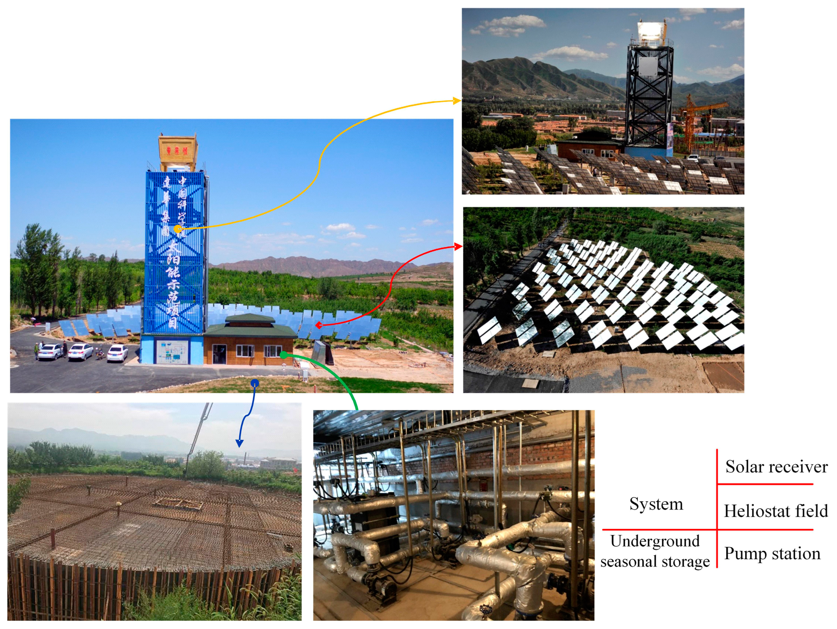
To fill the gaps mentioned above, based on a pilot solar-heating system with STS in Huangdicheng, northern China, a dynamic performance evaluation and operation strategy study are presented in this paper. The main novelties of the present study can be clarified as follows:

• The system’s dynamical performance was analyzed with a dynamic simulated method in typical-day or typical-operation modes, and the switch mechanism between multiple operation modes was revealed on a minute timescale;
• The system can reach a higher system performance with the proposed control strategies under different operation stages;
• The impacts of different heating operation strategies on the system performance were quantified. The performance indicators included the collection efficiency, storage efficiency, solar fraction of the system, and consumption of the circulation pump on the heating side.

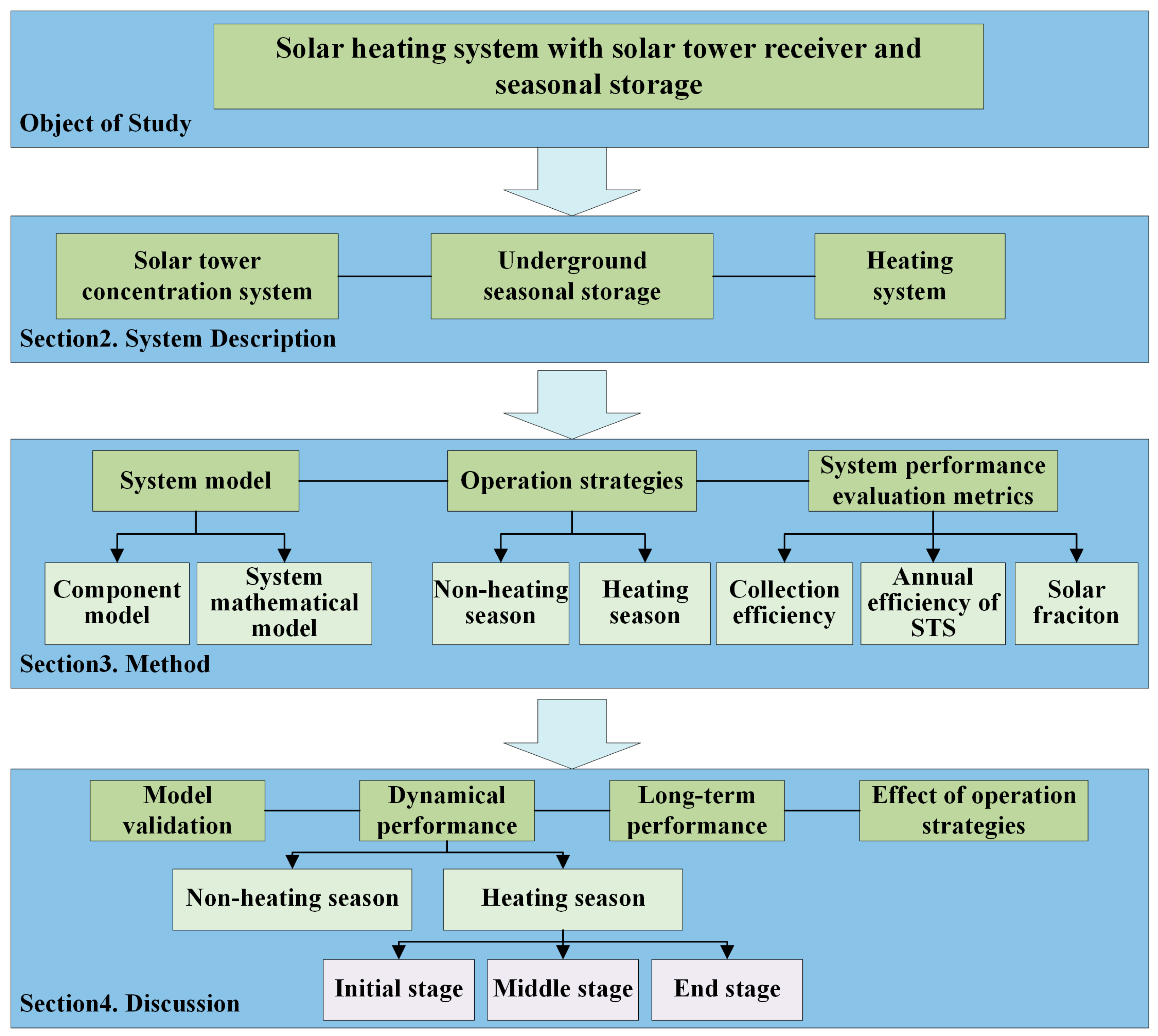
The frame structure of the study is presented in Figure 1. The concept of a pilot solar-heating system with a solar-tower receiver and STS is described in Section 2. Section 3 shows the analysis methods, which include the system simulation method, operation strategies, and performance evaluation metrics. Section 4 shows the validation of the system model, the assessment of the dynamic performance of the system in different operation modes, the long-term performance, and the analysis of the operation strategies. Finally, the main conclusions of our study are summarized in Section 5.

2. System Description

In this paper, a solar-heating system with STS (Figure 2) is studied based on a pilot project in Huangdicheng, Hebei, China (42.23° N, 115.43° E). The traditional flat-plate collectors in solar-heating systems have relatively low efficiencies at the typical supply temperatures of district-heating networks (70–95 °C) compared to concentrated solar thermal collectors [18]. This system adopts a concentrated solar-tower receiver to utilize the solar radiation, differing from the traditional solar-heating system. Underground-pit thermal storage was applied to solve the problem of the mismatch between the heat supply and demand in summer and winter. This water pit has 0.3 m thick concrete walls and was buried 1.0 m underground. The whole system consists of a concentrated solar thermal subsystem, an underground seasonal thermal storage unit, and a heating subsystem. A schematic of the system showing the main components is given in Figure 3. The parameters of the system are shown in

Table 1. System equipment parameters.

Program	Property	Quantity	Unit
Location	Latitude	40.23 N	°
	Longitude	115.43 E	°
Heliostat field	Number of heliostats	66
	Area of heliostats	11.2	m2
	Reflectivity	0.9
Solar receiver	Daylighting area	4.76	m2
Buffer tank	Volume	48	m3
Seasonal thermal storage	Volume	3000	m3
Heat exchanger	Area	30	m2

.

The complete operation cycle of the system is a year, which is divided into a heat-injection period (the local non-heating season) and a heat-extraction period (the heating season). The operating principle of the system is that in the heat-injection period, the concentrated solar thermal system charges for the STS; while, during the heat-extraction period, the concentrated solar thermal system (charging the buffer tank) and STS (discharging to the buffer tank) supply heat for the building [14].

3. Methodology

To analyze the dynamic performance of the system, mathematical models of the main component and the whole system were built, and the operation strategies were introduced under various operating modes.

3.1. System Model

The main components in this system include STS, a solar receiver, the heliostat field [14], circulation pumps, a buffer tank, and the building load. The dynamic model of the whole system was built based on the experimental system.

3.1.1. The Model of STS and the Solar-Receiver Model

The STS is a type of underground water pit in this system. The mathematical model is established based on the characteristics of the coupled heat transfer between the tank heat storage and soil. The STS model can be simplified to a one-dimensional model for the water body with a two-dimensional air layer on the top and a two-dimensional model for the soil and concrete wall. The developed model is validated in [19].

The solar receiver is a cavity receiver installed on a 30 m high tower. The model was established in MATLAB. Detailed descriptions of the model and validation are presented in [20].

3.1.2. Circulation-Pump Model

In this system, the collecting-side circulation pump, the circulation pumps on both sides of the heat exchanger, and the heating circulation pump are variable-speed pumps. To analyze the electricity consumption of the circulation pumps under different heating operating conditions, the power curves of the circulation pumps were added to the model, which were obtained via the least-squares method based on the performance parameters. The performance parameters of the pump were proposed by the equipment manufacturer.

The flow–power curve of the collecting-side circulation pump is calculated as follows:

$$P_p=0.0051F^2+0.052F+0.8416$$

(1)

The flow–power curve of the circulation pump on the primary side of the heat exchanger is calculated as follows:

$$P_p=0.00072F^2+0.0088F+1.3334$$

(2)

The flow–power curve of the circulation pump on the secondary side of the heat exchanger is calculated as follows:

$$P_p=-0.0041F^2+0.1421F-0.2232$$

(3)

The flow–power curve of the circulation pump on the heating side is calculated as follows:

$$P_p=-0.0000390F^2+0.05251F+2.7182$$

(4)

where $P_p$ (kJ/h) is the pump power, and $F$ (m³/h) is the flowrate of the pump.

3.1.3. Buffer-Tank Model

The buffer tank was assumed to be divided into multiple horizontal units. A multi-node heat-transfer model was established assuming that the working medium inside the node was completely mixed.

The energy-balance equation of each node in the buffer tank can be calculated as follows:

$${\rho }_{\mathrm{w}}{c}_{p,\mathrm{w}}{V}_i\frac{d{T}_{\mathrm{w},i}}{d\tau }=Q_{\mathrm{in},i}\left(\tau \right)-Q_{\mathrm{out},i}\left(\tau \right)-Q_{\mathrm{loss},i}\left(\tau \right)$$

(5)

where $Q_{\mathrm{loss},i}\left(\tau \right)$ is the heat loss caused by the heat dissipation between the surface of each node and the external environment, including through the top, side walls, and bottom of the buffer tank, and it can be calculated as follows:

$$Q_{\mathrm{loss},i}\left(\tau \right)=U_i{\mathrm{A}}_i\left(T_{\mathrm{w},i}-T_a\right)$$

(6)

where $U_i$ (W/(m² °C)) is the heat-loss coefficient of the buffer tank, and $A_i$ (m²) is the area of the surface of each node.

The heat and mass transfer of a node is shown in Figure 4, and the energy-balance equation can be expressed as follows:

$$\begin{array}{l}{\rho }_w{c}_{p,w}{V}_i\frac{d{T}_{w,i}}{d\tau }={\lambda }_w{A}_w\frac{\left(T_{w,i-1}-T_{w,i}\right)}{\Delta H}+{\lambda }_w{A}_w\frac{\left(T_{w,i}-T_{w,i+1}\right)}{\Delta H}+{\dot{m}}_i{c}_{p,w}\left(T_{w,i-1}-T_{w,i}\right)\\ \hspace{0.33em}\hspace{0.33em}\hspace{0.33em}\hspace{0.33em}\hspace{0.33em}\hspace{0.33em}\hspace{0.33em}\hspace{0.33em}\hspace{0.33em}\hspace{0.33em}\hspace{0.33em}\hspace{0.33em}+F_i^c{m}_h{c}_{p,w}\left(T_h-T_{w,i}\right)+F_i^d{m}_l{c}_{p,w}\left(T_l-T_{w,i}\right)-U_i{A}_i\left(T_{w,i}-T_a\right)\end{array}$$

(7)

where $\Delta H$ (m) is the height of the node; $T_h$ (°C) is the fluid temperature flowing into the buffer water tank on the load side; $m_h$, $m_l$ (kg/h) are the mass flows of the heat source and load side flowing into the buffer tank, respectively; $F_i{}^d$ is the control function, which determines whether the node is connected to the heat source or load side directly; $A_w$ (m²) is the outer surface area of the node.

The heat-loss coefficient of the buffer tank in our model was obtained through the experiment. The calculated formula can be represented as follows [21]:

$$U_i=\frac{M{c}_{p,w}\left(T_1-T_4\right)}{A\left(T_m-T_a\right)\Delta \tau }$$

(8)

where M is the mass of the water in the buffer tank (kg), $T_m$ (°C) is the average temperature of the buffer tank, $\Delta \tau$(s) is the total time length of n tests, and n is the number of tests.

3.1.4. Building-load model

The building load was modeled using the lumped-parameter method. The building energy-balance equation is calculated as follows [22]:

$$CAP\frac{d{T}_r}{d\tau }=\epsilon C_{\min }\left(T_i-T_r\right)+Q_{gain}-UA\left(T_r-T_a\right)$$

(9)

$$Q_T=\epsilon C_{\min }\left(T_i-T_r\right)$$

(10)

$$T_o=T_i-Q_T/m_h{c}_p$$

(11)

where $\epsilon$ is the heat-exchange efficiency of the heating coil at the end of the building; $CAP$ (kJ/K) is the effective lumped-heat capacity of the building; $C_{\min }$ (kJ/(h K)) is the minimum heat capacity in the heat-transfer fluid on both sides of the heat-exchange coil; $T_i$, $T_r$, $T_a$ (°C) are the heat-source temperature in the heat-exchange coil, the ambient temperature in the building, and the outdoor ambient temperature, respectively; $Q_{gain}$ is the heat increment from enclosures or windows; $UA$ (kJ/(h K)) is the heat-loss coefficient of the whole building; $Q_T$ is the total energy released by the heat source.

3.1.5. Mathematical Model of the Whole System

The mathematical models of every component are listed above, and the energy-transfer relationship between the core components and main parameters are presented in Figure 5. As shown, the system energy-transfer relationships are different under different operation modes. Thus, the mathematical equations of the whole system were established and solved according to the following four situations.

Situation 1: In the non-heating season, the solar-tower concentration system charges for the STS, and the energy-balance equation of the whole system can be represented as follows:

$$\left\{\begin{array}{l}{\rho }_{\mathrm{w}}{c}_{p,\mathrm{w}}{V}_{\mathrm{s}}\frac{d{T}_{\mathrm{w},s}}{d\tau }=Q_{\mathrm{in},\mathrm{s}}\left(\tau \right)-Q_{\mathrm{loss},\mathrm{s}}\left(\tau \right)\\ Q_{\mathrm{in},\mathrm{s}}\left(\tau \right)=Q_{\mathrm{rec},\mathrm{abs}}\left(\tau \right)=Q_{\mathrm{inc}}\left(\tau \right)-Q_{\mathrm{rec},\mathrm{loss}}\left(\tau \right)\\ Q_{\mathrm{inc}}\left(\tau \right)=Q_{\mathrm{solar}}\left(\tau \right)-Q_{\mathrm{h},\mathrm{loss}}\left(\tau \right)\\ Q_{\mathrm{inc}}\left(\tau \right)=Q_{\mathrm{solar}}\left(\tau \right)\cdot {\eta }_{\mathrm{h}}=N_{\mathrm{h}}\cdot A_{\mathrm{h}}\cdot I_{\mathrm{DNI}}\cdot {\eta }_{\mathrm{h}}\end{array}\right.$$

(12)

where $Q_{\mathrm{h},\mathrm{loss}}\left(\tau \right)$ is the energy loss of the heliostat field; $Q_{\mathrm{rec},\mathrm{abs}}\left(\tau \right)$ is the effective heat absorption of the solar receiver; $Q_{\mathrm{loss},\mathrm{s}}\left(\tau \right)$ is the heat loss of the STS; $Q_{\mathrm{solar}}(\tau )$ is the solar energy absorbed by the solar-tower concentration system; $Q_{\mathrm{inc}}\left(\tau \right)$ is the solar energy incident on the system.

Situation 2: In the non-heating season, the solar-tower concentration system charges for the buffer tank when the maximum temperature of the STS exceeds 90 °C. The energy-balance equation of the whole system can be expressed as follows:

$$\left\{\begin{array}{l}{\rho }_{\mathrm{w}}{c}_{p,\mathrm{w}}{V}_b\frac{d{T}_{\mathrm{w},\mathrm{b}}}{d\tau }=Q_{\mathrm{in},\mathrm{b}}\left(\tau \right)-Q_{\mathrm{loss},\mathrm{b}}\left(\tau \right)-Q_{\mathrm{supply},\mathrm{b}}\left(\tau \right)\\ Q_{\mathrm{in},\mathrm{b}}\left(\tau \right)=Q_{\mathrm{rec},\mathrm{abs}}\left(\tau \right)=Q_{\mathrm{inc}}\left(\tau \right)-Q_{\mathrm{rec},\mathrm{loss}}\left(\tau \right)\\ Q_{\mathrm{inc}}\left(\tau \right)=Q_{\mathrm{solar}}\left(\tau \right)-Q_{\mathrm{h},\mathrm{loss}}\left(\tau \right)\end{array}\right.$$

(13)

where $Q_{\mathrm{in},\mathrm{b}}\left(\tau \right)$ is the heat inputted to the buffer tank, $Q_{\mathrm{loss},\mathrm{b}}\left(\tau \right)$ is the heat loss of the buffer tank, and $Q_{\mathrm{supply},\mathrm{b}}\left(\tau \right)$ is the heat supplied by the buffer tank.

Situation 3: In the heating season, the solar-tower concentration system charges for the buffer tank. The buffer water tank supplies heat to the building directly when the heat of the buffer tank can meet the heat-load demand. The energy-balance equation of the whole system can be shown as follows:

$$\left\{\begin{array}{l}CAP\frac{d{T}_{\mathrm{r}}}{d\tau }=Q_{\mathrm{in},\mathrm{r}}\left(\tau \right)+Q_{\mathrm{gain},\mathrm{r}}\left(\tau \right)-Q_{\mathrm{loss},\mathrm{r}}\left(\tau \right)\\ Q_{\mathrm{in},\mathrm{r}}\left(\tau \right)=Q_{\mathrm{supply},\mathrm{b}}\left(\tau \right)=Q_{\mathrm{in},\mathrm{b}}\left(\tau \right)-Q_{\mathrm{loss},\mathrm{b}}\left(\tau \right)-{\rho }_{\mathrm{w}}{c}_{p,\mathrm{w}}{V}_b\frac{d{T}_{\mathrm{w},b}}{d\tau }\\ Q_{\mathrm{in},\mathrm{b}}\left(\tau \right)=Q_{\mathrm{rec},\mathrm{abs}}\left(\tau \right)=Q_{\mathrm{inc}}\left(\tau \right)-Q_{\mathrm{rec},\mathrm{loss}}\left(\tau \right)\\ Q_{\mathrm{inc}}\left(\tau \right)=Q_{\mathrm{solar}}\left(\tau \right)-Q_{\mathrm{h},\mathrm{loss}}\left(\tau \right)\end{array}\right.$$

(14)

where $Q_{\mathrm{in},\mathrm{r}}\left(\tau \right)$ is the heat input to the building, and $Q_{\mathrm{loss},\mathrm{r}}\left(\tau \right)$ is the heat loss of the building.

Situation 4: In the heating season, the solar-tower concentration system and the STS charge for the buffer tank. The buffer water tank provides heat for the building. When the heat of the buffer tank cannot meet the heat-load demand, the auxiliary heat source supplies heat to the buildings. The unsteady mathematical model of the system can be expressed as follows:

$$\left\{\begin{array}{l}CAP\frac{d{T}_{\mathrm{r}}}{d\tau }=Q_{\mathrm{in},\mathrm{r}}\left(\tau \right)+Q_{\mathrm{gain},\mathrm{r}}\left(\tau \right)-Q_{\mathrm{loss},\mathrm{r}}\left(\tau \right)\\ Q_{\mathrm{in},\mathrm{r}}\left(\tau \right)=Q_{\mathrm{supply},\mathrm{b}}\left(\tau \right)=Q_{\mathrm{in},\mathrm{b}}\left(\tau \right)-Q_{\mathrm{loss},\mathrm{b}}\left(\tau \right)-{\rho }_{\mathrm{w}}{c}_{p,\mathrm{w}}{V}_{\mathrm{b}}\frac{d{T}_{\mathrm{w},\mathrm{b}}}{d\tau }\\ Q_{\mathrm{in},\mathrm{b}}\left(\tau \right)=Q_{\mathrm{rec},\mathrm{abs}}\left(\tau \right)+Q_{\mathrm{discharge},\mathrm{s}}\left(\tau \right)+Q_{\mathrm{aux}}\left(\tau \right)\\ Q_{\mathrm{rec},\mathrm{abs}}\left(\tau \right)=Q_{\mathrm{solar}}\left(\tau \right)-Q_{\mathrm{h},\mathrm{loss}}\left(\tau \right)-Q_{\mathrm{rec},\mathrm{loss}}\left(\tau \right)\\ Q_{\mathrm{discharge},\mathrm{s}}\left(\tau \right)={\rho }_{\mathrm{w}}{c}_{p,\mathrm{w}}{V}_{\mathrm{s}}\frac{d{T}_{\mathrm{w},\mathrm{s}}}{d\tau }-Q_{\mathrm{loss},\mathrm{s}}\left(\tau \right)\end{array}\right.$$

(15)

where $Q_{\mathrm{aux}}\left(\tau \right)$ is the heat supplemented by an auxiliary heat source.

Each module is connected through the energy flow and combined with the system operation strategy. A solar-heating system with a solar-tower receiver and STS was finally built in TRNSYS 17.02 coupled with MATLAB. The dynamic operation characteristics and operation strategy of the system can be studied and analyzed on the platform. The system model is shown in Figure 6, and the descriptions of each module are shown in

Table 2. Main modules and parameters of the TRNSYS simulation platform.

Project	Name	Type	Notes
Meteorological parameters	Weather data	Type 15-3	Calling in typical annual meteorological data of Huailai obtained from the EnergyPlus website
Heliostat field	Hel	Type 394	Calling in instantaneous efficiency of the heliostat field
Receiver	Receiver	Type 155	Calling in structural parameters and mathematical models in MATLAB
Circulating pump	P (1~5)	Type 110	Inputting of the power curve of each circulation pump
Underground seasonal thermal storage	UGSTS	Type 207	Self-developed model
Buffer tank	Buffer tank	Type 531	Measured heat-loss coefficient: 0.34 W/(m2·°C)
Operation control unit	CON (1~3)	Type 2b	Temperature-difference control
	CONTROL	Calculator	Logical control
Data display or output	Plotter	Type 65d	Display of results
	Month result	Type 25c	Output of results
Diversion valve	D (1~4)	Type 11f	Switch between different circulation routes
Mixing valve	M (1~4)	Type 11d	Switch between different circulation routes
Heat exchanger	HE	Type 5b	Counterflow, average heat-transfer coefficient: 100 W/K per m2 of collector area [23]
Building load	LOAD	Type 12c	Heat load per unit of heating area: 40 W/m2
Heating season controller	SEASONAL	Type 14	The heating season is from November 1st to April 1st of the following year
Auxiliary fuel boiler	Boiler	Type 700	Rated power: 170 kW; boiler efficiency: 0.9
Temperature-control diverter valve	D5	Type 11b	The water-supply temperature can reach the set temperature by mixing the supply and return water

. The time step of the system model is 60 s [19]. The tolerance convergence of the system model is 0.001, and the working fluid in this system is pure water assuming incompressibility.

3.2. Operation Strategies

According to the performance of the main components and different operation modes, the control strategies are divided into the following situations.

3.2.1. Operation Strategy in the Non-Heating Season

In the constant-temperature-operation control strategy, the system performance is more prominent than the temperature-difference control in the non-heating season, as mentioned in [14]. Thus, the constant-temperature-operation control strategy was adopted in this study. The outlet temperature of the solar-tower concentration system was set to be 10 °C higher than the temperature of the top layer of the STS to prevent damage to the temperature stratification of the STS. By adjusting the flowrate of the circulation pump, the outlet temperature of the solar-tower concentration system can reach the set value.

3.2.2. Operation Strategy in the Heating Season

The solar-tower concentration system still worked with the constant-temperature-operation control strategy. The outlet temperature of the solar-tower concentration system was set to be 10 °C higher than the temperature of the top layer of the buffer tank.

The operation and regulation of the solar-heating system with STS is more complicated than the conventional heating system in the heating season. The temperature of the STS keeps decreasing in the heating season, and there is no heat pump in the system. The heat load decreased with the increase in the outdoor temperature at the beginning and end of the heating season, while the temperature of the STS was relatively high at the beginning of the heating season. Thus, there is an obvious mismatch between the heat-supply temperature and heat-demand temperature. This leads to many problems, including the waste of useful energy in the STS, significant heat loss in the pipelines, the destruction of temperature stratification in the STS, and a decrease in the efficiency of the solar-collection system. Therefore, it is necessary to propose a reasonable heating operation strategy. The control strategy of the heating circulation pump adopted the combination of quality–quantity regulation and staged variable-flow quality regulation in this study [24].

When the solar-tower concentration system is not operating or the heat collection of the solar-tower concentration system does not meet the heat demand, the STS will operate in the discharging mode. The discharge flowrate of the STS adopted the quantity regulation principle, which is the district heating regulation method [24]. Thus, the circulation pumps on both sides of the heat exchanger adopted the quantity regulation.

The circulation pump of the auxiliary heat source will start when the STS and solar-tower concentration system cannot meet the heat demand and constant-flow control is used.

3.3. System Performance Evaluation Metrics

1. The solar energy absorbed by the solar-tower concentration system can be calculated as follows:

$$Q_{\mathrm{solar}}={\displaystyle {\int }_{\tau 1}^{\tau 2}{N}_{\mathrm{h}}\cdot A_{\mathrm{h}}\cdot I_{\mathrm{DNI}}d\tau }$$

(16)

where $N_{\mathrm{h}}$ is the number of heliostats on the daylighting surface of the solar receiver at the current time, $A_{\mathrm{h}}$ (m²) is the aperture area of a single heliostat, and $I_{\mathrm{DNI}}$ (W/m²) is the direct normal irradiance.

2. The effective heat gain of the solar-tower concentration system can be calculated as follows:

$$Q_{col}={\displaystyle {\int }_{\tau 1}^{\tau 2}{c}_p\cdot m\cdot \left(T_{rec,ou\mathrm{t}}-T_{rec,in}\right)d}\tau$$

(17)

where $Q_{col}$ (J) is the heat effectively collected by the solar receiver; $c_p$ is the heat capacity of the water; m (kg/s) is the mass flow of the water; $T_{rec,in}$ (°C) is the inlet temperature of the solar receiver; $T_{rec,out}$ (°C) is the outlet temperature of the solar receiver.

3. The collection efficiency of the solar-tower concentration system can be calculated as follows:

$${\eta }_{\mathrm{col}}=\frac{Q_{col}}{Q_{solar}}$$

(18)

4. The annual efficiency of the STS can be expressed as follows:

$${\eta }_{\mathrm{n}}=1-\frac{Q_{loss}}{Q_{charge}}$$

(19)

$$Q_{charge}={\displaystyle {\int }_0^{\tau }{c}_p\cdot m\cdot \left(T_{in,s}-T_{out,s}\right)d}\tau$$

(20)

$$Q_{discharge}={\displaystyle {\int }_0^{\tau }{c}_p\cdot m\cdot \left(T_{out,s}-T_{in,s}\right)d}\tau$$

(21)

$$Q_{loss}=Q_{charge}-Q_{discharge}-Q_{st}$$

(22)

where $Q_{charge}$ is the heat charged into the STS; $Q_{discharge}$ is the heat discharged from the STS; $Q_{loss}$ is the heat loss of the STS; $Q_{st}$ is the energy change in the seasonal thermal energy storage; $T_{in,s}$ is the temperature of the water inflow during heat charging; $T_{out,s}$ is the temperature of the outflow water during heat charging.

5. The solar fraction can be expressed as follows [25]:

$$SF=\frac{Q_{sol}}{Q_{load}}$$

(23)

where $Q_{sol}$ is the heat supplied by solar energy for heating in the system, and $Q_{load}$ is the total heat load of the system.

4. Discussion

4.1. Model Validation

The models of the underground seasonal storage and solar receiver are validated in [19,20]. The measured data from 1 October 2018 to 7 October 2018 were selected to verify the system simulation model. Because the solar-tower concentration system charges for the STS in actual operation, the inlet and outlet temperatures of the solar receiver and the internal temperature distribution of the STS are used for comparison between the experiment and simulation. The root-mean-square deviation (RMSD), average relative errors (ARE), and maximum relative errors (MRE) are listed in

Table 3. Root-mean-square deviations, average relative errors, and maximum relative errors of numerical results.

Location	RMSD (°C)	ARE (%)	MRE (%)
T1 (4.25 m from STS bottom)	1.10	0.42	1.52
T2 (3.45 m from STS bottom)	1.54	0.75	1.85
T3 (2.65 m from STS bottom)	0.79	0.45	0.28
T4 (1.85 m from STS bottom)	0.32	0.03	0.57
T5 (1.05 m from STS bottom)	1.23	0.75	1.63
T6 (0.25 m from STS bottom)	0.50	0.12	0.92
Inlet temperature of receiver	1.12	2.49	6.0
Outlet temperature of receiver	3.01	2.57	9.8

.

$$\mathrm{RMSD}=\sqrt{\frac{{\displaystyle {\sum }_{j=1}^N(T_{j,\exp }-T_{j,sim})}}{N}}$$

(24)

$$\mathrm{ARE}=\frac{1}{N}{\displaystyle \sum _{j=1}^N\frac{(T_{j,\exp }-T_{j,sim})}{T_{j,\exp }}}\times 100\%$$

(25)

$$\mathrm{MRE}=MAX\left(\frac{\left|T_{j,\exp }-T_{j,sim}\right|}{T_{j,\exp }}\right)\times 100\%$$

(26)

In this study, the measured parameters are the temperatures and flowrates. The uncertainties of the above parameters are calculated as follows [26]:

$$\delta R=\sqrt{{\displaystyle {\sum }_i^N{\left(\frac{\mathsf{\partial }R}{\mathsf{\partial }{X}_i}\delta X_i\right)}^2}}$$

(27)

where R and δR are the measured parameter and the uncertainty, respectively. X_i and δX_i are the measurement value and the accuracy of the test equipment, respectively. The accuracies of the test equipment and the uncertainties of the experimental results are shown in

Table 4. Test equipment and specifications.

Measurement Device	Type	Range	Accuracy
Temperature sensor	PT100	0~100 °C	±0.5 °C
Vortex flowmeter	HH-HYBLWGY-50	0~25 m3/h	±1.0%

and

Table 5. The uncertainties of the experimental results.

Parameter	Type of Data	Unit	Relative Error
Average inlet temperature of solar receiver	Measured	°C	3.783%
Average outlet temperature of solar receiver	Measured	°C	2.049%
Average flowrate	Measured	m3/h	1.058%
Average temperature of STS	Measured	°C	0.983%

, respectively.

The comparisons of the experimental results and simulation of the inlet and outlet temperatures of the solar receiver are shown in Figure 7. The results show that the measured values of the outlet temperature of the solar receiver were in good agreement with the simulated values for a continuous week. The simulation results were slightly different from the experimental values only when the circulation pump started and stopped. The reason was that the heat transfer caused by the oscillating flow in the receiver tubes was not considered in the simulation model when the circulation pump started and stopped. However, the maximum deviation of the inlet and outlet temperatures of the solar receiver was not greater than 3 °C, and the average error of the outlet temperature was 2.57%. Thus, the overall simulation model can reflect the dynamic operation performance of the solar receiver under different weather conditions.

The comparations of the experimental results and simulation values of the temperature at different heights in the STS are shown in Figure 8. The simulation results agreed well with the experimental values. There were some deviations between the simulated values and the experimental values at the top two measurement points. The reason was that soil moisture is affected by the environmental temperature and humidity, which has a certain impact on the heat transfer between water and soil. However, this was not considered in this model. The maximum deviation between the experimental value and the simulated value of the temperature in each layer was not greater than 1.0 °C, and the maximum error was 1.85%.

The results indicated that the simulated values of the system were in good agreement with the experiment values. Therefore, the system model can accurately reflect the dynamic operation characteristics and performance of the system.

4.2. Dynamical Performance of the System

Due to the instability of solar radiation and the heat demand of buildings, solar-heating systems work under variable working conditions. The dynamical performance was analyzed with a dynamic simulated method in typical-day or typical-operation modes, and the switch mechanism between multiple operation modes was also revealed.

The local typical yearly meteorological data and the heat demand of the 3000 m² building, which were calculated via the system model, are shown in Figure 9. The annual heat load of the system was 1,571,976.2 MJ. Solar radiation was relatively low from October to March of the next year. This is also the local heating season. The total horizontal solar radiation and the ambient temperature reached the minimum around January, while the building heat load reached the maximum. The total horizontal solar irradiation is relatively high in the rest of the year, during which there is no heat demand. Therefore, there is a serious mismatch between solar resources and demand. This means that there is a waste of solar energy in the summer and a lower solar fraction, which is the typical problem of solar-heating systems in northern China. The solar-heating system with STS in this paper can effectively solve the above problems. Moreover, the system has the advantages of reducing heating costs and achieving stable, continuous operation with high efficiency.

4.2.1. Dynamic Characteristic Analysis of Typical Working Conditions in the Non-Heating Season

In the non-heating season, the working fluid is pumped from the bottom of the STS to the solar-tower concentration system, and it is then heated by the solar receiver and charged to the top of the STS. The dynamic operation characteristics of the solar-tower receiver on a typical day and the temperature-change process of the STS over a continuous week were analyzed with minute-level-measured meteorological data. The inlet temperature of the solar receiver and the top temperature of the STS were set to 60 °C and 80 °C, respectively. In constant-temperature mode, the outlet temperature of the solar receiver was set to 10 °C higher than the top temperature of the STS. The dynamic performance of the solar receiver on a typical day is shown in Figure 10. The typical day was cloudy, and the maximum DNI of the whole day was 550 W/m². Severe fluctuations in solar radiation occurred around 3:30 p.m. owing to the influence of clouds. Therefore, the flowrate of the circulation pump of the solar receiver fluctuated greatly when the solar radiation changed violently. When the solar irradiance fluctuates, it is necessary to continuously adjust the flowrate of the solar-receiver circulation pump to ensure that the outlet temperature of the solar receiver reaches the set temperature. As shown in Figure 10, the changing trend of the flowrate was consistent with that of the DNI. The outlet temperature of the solar receiver remained around 90 °C throughout the day, which was 10 °C higher than the temperature of the STS.

As shown in Figure 11, the solar-tower concentration system ran continuously for one week in constant-temperature mode, and the dynamic performances of the solar receiver and STS were presented. The measured temperature stratification of the STS was imported as the initial condition. Regardless of the various solar irradiation conditions, such as cloudy or sunny, the solar receiver can maintain a good operating state during continuous operation for one week. The outlet temperature of the solar receiver was ensured to be 10 °C higher than the top temperature of the STS by dynamically adjusting the circulation-pump flowrate under different solar irradiation conditions. The temperature stratification in the STS was maintained well, and the temperature of each layer kept rising. Due to the proximity of the charging port to the top layer and the high charging temperature, the top-layer temperature rose more obviously than that of the bottom layer. As a consequence, the temperature stratification in the STS was effectively improved. Temperature stratification is one of the important criteria for evaluating the performance of sensible heat storage, and it determines the efficiency of the STS and the entire solar-heating system. Good temperature stratification not only improves the available heat of the system, but it also plays an important role in improving the heat-collection efficiency of the solar-tower concentration system and reducing the heat loss of the STS.

4.2.2. Dynamic Characteristic Analysis of Typical Working Conditions in the Heating Season

The operation performance of the solar-heating system must be evaluated on the premise of satisfying a continuous and stable energy supply and ensuring the thermal comfort of users. The solar fraction and heating stability of the solar-heating system are effectively improved by STS. The operation state of the system in the heating season is more complex than that in the non-heating season. The STS, which is a supplementary heat source, has a higher temperature in the initial stage of the heating season, while the required heating temperature is lower. The supply and required heating temperatures do not match, and the temperature of the STS gradually decreases. For the above operating characteristics, the heating season is divided into the initial stage, the middle stage, and the end of the heating season. The dynamic operation characteristics of the STS under different operating conditions and the switching mechanisms of multiple modes were analyzed.

1.

In the initial stage of the heating season

During this period, the outdoor ambient temperature and the temperature in the STS are both high, while the building load and the required heating temperature are both low. The solar-tower concentration system can basically meet the building load. The STS supplies heat to the buildings through heat exchangers when the solar radiation is poor or when there is no solar radiation. The minute-level-measured meteorological data of two consecutive days (27–28 November 2018) were selected to analyze the dynamic operation performance of the system. The initial temperature of the buffer water tank was set to 35 °C, and the top temperature of the STS water was set to 80 °C. Based on the heating-control strategy proposed in this study, the heating-supply temperature of the system was adjusted with the change in the ambient temperature. The supply temperature increased when the outdoor ambient temperature decreased.

As shown in Figure 12, as the outdoor ambient temperature decreased, the building heat load increased accordingly. There were three discharge times of the STS during the two consecutive days. The solar-tower concentration system stopped running after 5 p.m. The buffer tank was used for heating preferentially. When the temperature of the upper layer of the buffer tank dropped to 5 °C higher than the supply temperature, the STS started to charge for the buffer tank until the upper-layer temperature rose to 15 °C higher than the supply temperature in order to ensure the stability of the system heating and reduce the starting and stopping times of the circulation pump of the STS. Furthermore, when the outdoor environment temperature increases, the discharge power of the STS will decrease to achieve the efficient and reasonable utilization of the stored heat. The system can continuously and stably supply heat under the dynamic changes in the solar radiation resources and building load. The indoor temperature of the building was maintained at around 20 °C, which basically met the thermal comfort of users.

2.

In the middle stage of the heating season

The middle stage of the heating season refers to the time when the outdoor ambient temperature basically reaches the lowest and the heat load reaches the highest throughout the year, and the temperature of the STS continuously decreases to the required water-supply temperature. The solar-tower concentration system heats the building directly, basically meeting the heat demand when the solar radiation is good. Minutely measured meteorological data on 20 January 2018 were selected to analyze the dynamic operation of the system heating. The initial temperature of the buffer tank was set at 45 °C.

The heating-control strategy of the system in the middle stage of the heating season is the same as that in the initial stage. As shown in Figure 13, when the temperature of the top layer of the STS dropped to only 1 °C higher than the supply temperature, the auxiliary boiler was used to supplement the heat until the temperature of the upper layer of the buffer tank was higher than the supply temperature or the solar-tower concentration system started. In the middle of the heating season, it is mainly affected by the dynamic changes in the solar radiation resources, building load, and discharging temperature of the STS. There were three operation modes: the direct heating of the solar-tower concentration system, discharging of the STS, and auxiliary-boiler heating. The system could supply heat continuously and stably, and the indoor temperature of the building was kept at about 20 °C.

3.

At the end of the heating season

At the end of the heating season, the outdoor ambient temperature gradually increases, and the heat-load and -supply temperatures gradually decrease. At the same time, the temperature of the STS may still be higher than the supply temperature, although it continues to decline. Minute-level-measured meteorological data for two consecutive days (1–2 March 2019) were selected to analyze the dynamic performance of the system. The initial temperature of the buffer tank was set at 45 °C.

The system heating regulation strategy at the end of the heating season was the same as that of the above stages. The solar-tower concentration system provided heat to the buffer tank when the solar radiation was sufficient. When the solar-tower concentration system stopped running, the heat stored in the buffer tank was used preferentially for heating after 5:00 p.m. on 1 March. It was cloudy on 2 March, and the direct heating of the solar-tower concentration system basically met the heat demand. When the temperature of the upper layer of the buffer tank dropped to 5 °C higher than the supply temperature, the STS was used as a heat supplement, such as at around 2:00 a.m. on 1 March, as shown in Figure 14. Between 3:00 a.m. and 8:00 a.m., the auxiliary boiler ran until the start of the solar-tower concentration system. There were three operation modes to switch: the direct heating of the solar-tower concentration system, discharging of the STS, and auxiliary-boiler heating.

4.3. Long-Term Performance of the System

To analyze the dynamic performance in different time dimensions, the operating characteristics of the system for one year and three consecutive years were simulated with the typical local meteorological data. The initial temperatures of the STS and the surrounding soil were set to 14 °C and 8 °C, respectively, according to the measured data. The simulation results of the outlet temperature of the solar receiver and the temperature change of the STS in the first year are shown in Figure 15.

In the non-heating season, the average temperature of the STS increased from 14.0 °C to 84.7 °C, and it dropped to 35.9 °C until the end of the heating season. To avoid damaging the temperature stratification in the STS, the outlet temperature of the solar receiver was set to be higher than the water temperature at the top of the STS, approaching 90 °C at the end of the non-heating season (from August to October). In the heating season, the operating temperature of the solar receiver was affected by the buffer tank. The outlet temperature of the solar receiver was set to be higher than the supply temperature, and the buffer tank basically met the heat demand at the end of the heating season. As a result, the solar receiver also operated at a higher temperature. The traditional flat-plate collectors in solar-heating systems have relatively low efficiencies at the typical supply temperatures of district-heating networks (70–95 °C) compared to the concentrated solar thermal collectors. Thus, the solar-tower concentration system in this paper has certain advantages at the end of the non-heating season and in the heating season.

The energy flow of the solar-heating system in the first year is shown in Figure 16. The solar-tower concentration system collected 591.6 MWh of heat in the whole year, and the annual average thermal efficiency was 50.2%. In the non-heating season, with the gradual increase in the storage capacity and average temperature of the STS, the heat loss also increased. In September and October, due to the lower DNI and the higher operating temperatures of the solar receiver and the STS, the heat collection increased less, and the heat loss of the STS increased. In the heating season, the solar-tower concentration system supplied heat to users by charging the buffer tank. At the beginning of the heating season (November and December), the heat supplied by the heat-collection system and STS could meet the heat demand, and the solar fraction reached 100%. In the middle of the heating season (January), the auxiliary heat source supplemented 25.3 MWh in January. At the end of the heating season (February and March), the heating temperature required by the user side was relatively low. The supplementary heat of the auxiliary heat source was less, with 9.7 MWh. Most of the heat came from the solar-tower concentration system. The annual solar fraction of the system can reach 85.9% with 375.1 MWh, and the annual efficiency of the STS is 56.1%. Furthermore, the heat stored in the STS can be effectively extracted throughout the heating season.

The temperature changes of the STS for three consecutive years are shown in Figure 17. It shows that the average temperature of the STS at the end of the heating season was 35.9 °C in the first year. In the second year, the initial temperature of the STS and the operating temperature of the system were higher at the end of the non-heating season. The annual average efficiency of the solar-tower concentration system and the heat charging to the STS in the second and third years gradually decreased.

As shown in Figure 18, the heat discharged from the STS increased year by year. In the third year, the discharged heat reached 186.1 MWh, and the annual storage efficiency was 57.5%. The temperature of the soil gradually improved and reached an equilibrium state. It was remarkable that a heat pump was not added to this system, and that the heat in the STS was not completely used up in the first year. This led to a higher initial temperature in the second year. Furthermore, the solar fraction of the system was gradually improved. The solar fraction of the system reached 89.4% in the third year, which was 3.6% higher than that in the first year.

4.4. Effects of Operation Strategies

The impacts of different heating operation strategies on the system performance were analyzed. This included quantity regulation, quality regulation, constant-temperature and -flowrate regulation, and the quantity–quality regulation that is proposed in this paper. The influence of the heating strategy was assessed via the performance indicators, such as the collection efficiency, storage efficiency, solar fraction of the system, and consumption of the circulation pump on the heating side. The heat discharged by the STS needs to be effectively utilized to realize the stable heating of the system during the heating season. However, the temperature of the STS gradually decreased during the operation. If the quantity regulation and constant-temperature and -flow heating-control modes were adopted, then the heating temperature was always set to a constant-temperature operation (such as 55 °C). In addition, if the heat pump or reheating method is not used, then the heat stored in the STS cannot be effectively used, and the STS is in a static heat-dissipation state when its temperature drops below 55 °C. As a result, the solar fraction and annual efficiency of the STS are lower, and the electricity consumption of the circulation pump with quantity regulation is lower than that with constant-temperature and -flow regulation (Figure 19). The quality regulation and quantity–quality regulation improved the solar fraction and annual average efficiency of the solar-tower concentration system compared with the other two methods. The heat stored in the STS could be fully utilized, and the heat loss of the pipe network could be reduced. The electricity consumption of the pump was 18.4 MWh in the quality control. However, when the quantity–quality regulation method was adopted, it was significantly reduced to 10.2 MWh, a reduction of 44.6%. The solar fraction of the system was also 17.5% higher than that of the constant-temperature and -flowrate control.

As shown in Figure 20, in the quantity–quality regulation strategy, the STS discharged heat every month during the heating season. The solar fraction of the system reached 100% in November and December. The heat discharged from the STS accounted for 13% of the total heat supply in March of the next year. However, under the constant-temperature and -flowrate mode, the solar fraction of the system reached 100% only in November, and the STS discharged heat only in November and December, accounting for 58% of the heat supply in these months.

5. Conclusions

A pilot solar-heating system with a solar-tower receiver and STS was established. The dynamic performances of the system at different time scales were studied. Furthermore, a comparative study was conducted to investigate the influences of the operation strategies. The main conclusions are as follows:

(1)

The solar-heating system with STS in our study had an outstanding performance at different time scales. Through the switching of multiple operation modes, the system can operate stably and continuously under fluctuations in solar radiation resources and the heat demand. The significant mismatch between the solar energy and heat load in northern China can be resolved;

(2)

The quality–quantity operation strategies are effective ways to improve the discharge efficiency of the STS and the system performance without a heat pump to utilize the thermal energy stored in the STS when the temperature of the STS is below the traditional heating-supply temperature. The annual solar fraction of the system could reach 85.9%, and the annual efficiency of the STS was 56.1%. The electricity consumption of the pump on the heating side could be significantly reduced by 44.6% compared with the quality control;

(3)

The solar fraction of the system was gradually improved. The solar fraction of the system reached 89.4% in the third year, which was 3.6% higher than that in the first year. Although the solar-tower collection system can improve the collection efficiency at a higher temperature, the operational temperature still affects the system performance, especially in the third year. Thus, reasonable control strategies for the whole system should be analyzed in different time dimensions, such as the long-term period;

(4)

In order to promote the development of solar-heating systems with STS, scientific design methods for system configuration and operation strategies need to be addressed in the future. Based on perfect forecasts of the weather and SDH loads, the development of optimized control strategies is the focus of future research.

References

1. Annual Development Research Report on Building Energy Efficiency in China 2022; Tsinghua University Building Energy Efficiency Research Center: Beijing, China, 2022; pp. 1–23.
2. Rghif, Y.; Zeghmati, B.; Bahraoui, F. Numerical Analysis of the Influence of Buoyancy Ratio and Dufour Parameter on Thermosolutal Convection in a Square Salt Gradient Solar Pond. Fluid Dyn. Mater. Process. 2022, 18, 1319–1329. [Google Scholar] [CrossRef]
3. Rghif, Y.; Zeghmati, B.; Bahraoui, F. Modeling the Influences of a Phase Change Material and the Dufour Effect on Thermal Performance of a Salt Gradient Solar Pond. Int. J. Therm. Sci. 2021, 166, 106979. [Google Scholar] [CrossRef]
4. Rghif, Y.; Bahraoui, F.; Zeghmati, B. Experimental and Numerical Investigations of Heat and Mass Transfer in a Salt Gradient Solar Pond under a Solar Simulator. Sol. Energy 2022, 236, 841–859. [Google Scholar] [CrossRef]
5. Rghif, Y.; Colarossi, D.; Principi, P. Effects of Double-Diffusive Convection on Calculation Time and Accuracy Results of a Salt Gradient Solar Pond: Numerical Investigation and Experimental Validation. Sustainability 2023, 15, 1479. [Google Scholar] [CrossRef]
6. Tosatto, A.; Dahash, A.; Ochs, F. Simulation-Based Performance Evaluation of Large-Scale Thermal Energy Storage Coupled with Heat Pump in District Heating Systems. J. Energy Storage 2023, 61, 106721. [Google Scholar] [CrossRef]
7. Narula, K.; De Oliveira, F.; Villasmil, W.; Patel, M.K. Simulation Method for Assessing Hourly Energy Fl Ows in District Heating System with Seasonal Thermal Energy Storage. Renew. Energy 2020, 151, 1250–1268. [Google Scholar] [CrossRef]
8. Ushamah, H.M.; Ahmed, N.; Elfeky, K.E.; Mahmood, M.; Qaisrani, M.A.; Waqas, A.; Zhang, Q. Techno-Economic Analysis of a Hybrid District Heating with Borehole Thermal Storage for Various Solar Collectors and Climate Zones in Pakistan. Renew. Energy 2022, 199, 1639–1656. [Google Scholar] [CrossRef]
9. Kim, M.H.; Kim, D.; Heo, J.; Lee, D.W. Techno-Economic Analysis of Hybrid Renewable Energy System with Solar District Heating for Net Zero Energy Community. Energy 2019, 187, 115916. [Google Scholar] [CrossRef]
10. Chu, S.; Sethuvenkatraman, S.; Goldsworthy, M.; Yuan, G. Techno-Economic Assessment of Solar Assisted Precinct Level Heating Systems with Seasonal Heat Storage for Australian Cities. Renew. Energy 2022, 201, 841–853. [Google Scholar] [CrossRef]
11. Renaldi, R.; Friedrich, D. Techno-Economic Analysis of a Solar District Heating System with Seasonal Thermal Storage in the UK. Appl. Energy 2019, 236, 388–400. [Google Scholar] [CrossRef] [Green Version]
12. Zhang, C.; Nielsen, E.; Fan, J.; Furbo, S. Thermal Behavior of a Combi-Storage in a Solar-Ground Source Heat Pump System for a Single-Family House. Energy Build. 2022, 259, 111902. [Google Scholar] [CrossRef]
13. Maragna, C.; Rey, C.; Perreaux, M. A Novel and Versatile Solar Borehole Thermal Energy Storage Assisted by a Heat Pump. Part 1: System Description. Renew. Energy 2023, 208, 709–725. [Google Scholar] [CrossRef]
14. Li, X.; Wang, Z.; Li, J.; Yang, M.; Yuan, G.; Bai, Y. Comparison of Control Strategies for a Solar Heating System with Underground Pit Seasonal Storage in the Non-Heating Season. J. Energy Storage 2019, 26, 100963. [Google Scholar] [CrossRef]
15. Villasmil, W.; Troxler, M.; Hendry, R.; Schuetz, P.; Worlitschek, J. Control Strategies of Solar Heating Systems Coupled with Seasonal Thermal Energy Storage in Self-Sufficient Buildings. J. Energy Storage 2021, 42, 103069. [Google Scholar] [CrossRef]
16. Wang, Y.; Rao, Z.; Liu, J.; Liao, S. An Optimized Control Strategy for Integrated Solar and Air-Source Heat Pump Water Heating System with Cascade Storage Tanks. Energy Build. 2020, 210, 109766. [Google Scholar] [CrossRef]
17. Zhao, J.; Lyu, L.; Li, X. Numerical Analysis of the Operation Regulation in a Solar Heating System with Seasonal Water Pool Thermal Storage. Renew. Energy 2020, 150, 1118–1126. [Google Scholar] [CrossRef]
18. Tian, Z.; Perers, B.; Furbo, S.; Fan, J. Annual Measured and Simulated Thermal Performance Analysis of a Hybrid Solar District Heating Plant with Flat Plate Collectors and Parabolic Trough Collectors in Series. Appl. Energy 2017, 205, 417–427. [Google Scholar] [CrossRef] [Green Version]
19. Bai, Y.; Wang, Z.; Fan, J.; Yang, M.; Li, X.; Chen, L.; Yuan, G.; Yang, J. Numerical and Experimental Study of an Underground Water Pit for Seasonal Heat Storage. Renew. Energy 2020, 150, 487–508. [Google Scholar] [CrossRef]
20. Li, X.; Wang, Z.; Li, J.; Chen, L.; Bai, Y.; Yang, M.; Guo, M.; Sun, F.; Yuan, G. Numerical and Experimental Study of a Concentrated Solar Thermal Receiver for a Solar Heating System with Seasonal Storage. Int. J. Energy Res. 2021, 45, 7588–7604. [Google Scholar] [CrossRef]
21. GB/T18708-2002; Test Methods for Thermal Performance of Domestic Solar Water Heating System. General Administration of Quality Supervision, Inspection and Quarantine of the China: Beijing, China, 2002.
22. University of Wisconsin-Madison. Volume 4: Mathematical Reference. In TRNSYS 17 Manual; Solar Energy Laboratory, University of Wisconsin-Madison: Madison, WI, USA, 2009. [Google Scholar]
23. Pahud, D. Central solar heating plants with seasonal duct storage and short-term water storage: Design guidelines obtained by dynamic system simulations. Sol. Energy 2000, 69, 495–509. [Google Scholar] [CrossRef]
24. Xiaoxia, L.; Zhifeng, W.; Jinping, L.; Yang, M.; Bai, Y.; Chen, L. Space Heating Management for Solar Heating System with Underground Pit Storage; Springer: Singapore, 2020; Volume III, ISBN 9789811395277. [Google Scholar]
25. Ciampi, G.; Rosato, A.; Sibilio, S. Thermo-Economic Sensitivity Analysis by Dynamic Simulations of a Small Italian Solar District Heating System with a Seasonal Borehole Thermal Energy Storage. Energy 2018, 143, 757–771. [Google Scholar] [CrossRef]
26. Moffat, R.J. Describing the Uncertainties in Experimental Results. Exp. Therm. Fluid Sci. 1988, 1, 3–17. [Google Scholar] [CrossRef] [Green Version]
Figure 1. Frame structure of this paper.
Energies 16 05505 g001
Figure 2. Solar-heating system with STS and solar receiver.
Energies 16 05505 g002
Figure 3. Schematic of solar-heating system. (The dashed lines represent the signal flow, while the solid lines represent the heat and mass flow).
Energies 16 05505 g003
Figure 4. Energy transfer at node of buffer tank.
Energies 16 05505 g004
Figure 5. Transfer relationship of energy flow of core components.
Energies 16 05505 g005
Figure 6. TRNSYS simulation platform for the solar-heating system. (The dashed lines represent the signal flow, while the solid lines represent the heat and mass flow).
Energies 16 05505 g006
Figure 7. Simulated and measured inlet and outlet temperatures of solar-tower concentration system.
Energies 16 05505 g007
Figure 8. Experimental and simulation values of temperature at different heights in STS (S: simulation; M: measured).
Energies 16 05505 g008
Figure 9. Local typical annual meteorological data and heating load.
Energies 16 05505 g009
Figure 10. Dynamic operation performance of solar receiver on a typical day.
Energies 16 05505 g010
Figure 11. Performance of continuous operation for one week.
Energies 16 05505 g011
Figure 12. Dynamic operation performance at beginning of heating season.
Energies 16 05505 g012
Figure 13. Dynamic operation performance in the mid-heating season.
Energies 16 05505 g013
Figure 14. Dynamic operation performance at the end of the heating season.
Energies 16 05505 g014
Figure 15. Annual operation performance of the system.
Energies 16 05505 g015
Figure 16. Operation energy flow in the first year.
Energies 16 05505 g016
Figure 17. Temperature changes of STS for three consecutive years.
Energies 16 05505 g017
Figure 18. System performance change over three continuous years.
Energies 16 05505 g018
Figure 19. System performance under different heating strategies.
Energies 16 05505 g019
Figure 20. Contribution rates of different heat sources. (a) Quantity–quality regulation. (b) Constant temperature and flowrate.
Energies 16 05505 g020aEnergies 16 05505 g020b