Article

Impedance Acquisition of Proton Exchange Membrane Fuel Cell Using Deeper Learning Network

1
School of Automotive Studies, Tongji University, Shanghai 201804, China
2
Haidriver (Qingdao) Energy Technology Co., Ltd., Qingdao 266199, China
3
Postdoctoral Station of Mechanical Engineering, Tongji University, Shanghai 201804, China
*
Author to whom correspondence should be addressed.
Energies 2023, 16(14), 5556; https://doi.org/10.3390/en16145556
Submission received: 21 June 2023 / Revised: 12 July 2023 / Accepted: 20 July 2023 / Published: 22 July 2023
(This article belongs to the Section A5: Hydrogen Energy)

Abstract

:
Electrochemical impedance is a powerful technique for elucidating the multi-scale polarization process of the proton exchange membrane (PEM) fuel cell from a frequency domain perspective. It is advantageous to acquire frequency impedance depicting dynamic losses from signals measured by the vehicular sensor without resorting to costly impedance measurement devices. Based on this, the impedance data can be leveraged to assess the fuel cell’s internal state and optimize system control. In this paper, a residual network (ResNet) with strong feature extraction capabilities is applied, for the first time, to estimate characteristic frequency impedance based on eight measurable signals of the vehicle fuel cell system. Specifically, the 2500 Hz high-frequency impedance (HFR) representing proton transfer loss and 10 Hz low-frequency impedance (LFR) representing charge transfer loss are selected. Based on the established dataset, the mean absolute percentage errors (MAPEs) of HFR and LFR of ResNet are 0.802% and 1.386%, respectively, representing a superior performance to other commonly used regression and deep learning models. Furthermore, the proposed framework is validated under different noise levels, and the findings demonstrate that ResNet can attain HFR and LFR estimation with MAPEs of 0.911% and 1.610%, respectively, even in 40 dB of noise interference. Finally, the impact of varying operating conditions on impedance estimation is examined.

1. Introduction

The development of new energy vehicles has an influential impact on global energy security and environmental protection, with fuel cell vehicles being a potential contender for the next generation due to their zero emissions, quick hydrogenation time, and extended driving range. Of the various fuel cells, the proton exchange membrane (PEM) fuel cell is largely utilized in the field of transportation because of its high energy density, rapid dynamic response, and high conversion efficiency [1]. However, the large-scale commercial application of the PEM fuel cell is still impeded by its durability. In complex vehicle conditions, improper membrane water content, liquid water content, and oxygen concentration of the PEM fuel cell can lead to drying, flooding, and starvation, necessitating real-time estimation of the internal state of the PEM fuel cell and conducting IT-based feedback control to effectively avert or alleviate the occurrence of these faults, and enhance its output performance and service life [2].
There is a prevailing desire to precisely ascertain the internal state of fuel cells using in-vehicle sensors. Due to the closed structure of fuel cells, the conventional external measurement signals, including temperature, pressure, flow, voltage, and others, are often amalgamated with the lumped parameter model of the fuel cell to create a state observer for estimating the internal state [3]. Nevertheless, establishing a precise fuel cell model for intricate vehicle operating conditions is often unattainable. On the other hand, the electrochemical impedance, which is reflective of the polarization process of fuel cells in the frequency domain, can quantitatively measure the polarization loss [4]. To date, electrochemical impedance has been extensively employed for the purpose of fuel cell performance characterization and fault diagnosis [5]. High-frequency impedance, indicative of proton transfer and ohmic loss, is an effective indicator of membrane water content, and thus can be utilized in the management of shutdown purging and diagnosing membrane drying [6]. Additionally, mid-frequency capacitance loops caused by charge transfer and low-frequency capacitance loops determined by humidity-dependent ionomer properties are important for water management to prevent flooding faults [7]. Specific low-frequency information indicating oxygen transfer and storage in the catalyst layer can further assist with air starvation diagnosis [8]. Therefore, electrochemical impedance can be considered a reliable supplementary signal for identifying the internal state of fuel cells. Online acquisition of fuel cell impedance makes it possible to adjust operating conditions promptly to ensure that the internal state remains within an acceptable range, thus facilitating the development of an advanced fuel cell management system.
The impedance is usually measured by the electrochemical workstation, which is not easy to obtain online in a vehicle fuel cell system, limited by the equipment price, interference, and measured time. To address this limitation, various online impedance acquisition methods for PEM fuel cells have been proposed. Initially, the equivalent circuit model (ECM) comprising resistors and capacitors was used to approximate polarization loss by fitting the current and voltage data [9,10]. However, ECM is unable to accurately simulate the voltage overshoot caused by membrane water redistribution during loading. Additionally, both impedance dimension and impedance process models are too complex to be implemented online [11]. To improve the accuracy and efficiency of online impedance acquisition, some researchers have adopted harmonic excitation signals in conjunction with time-frequency analysis methods to calculate broadband impedance spectrums quickly. This technical path is feasible because the excitation signal with rich harmonic information can be superimposed by approximately infinite sinusoidal excitation with different frequencies. Examples include Chirp excitation with short-term Fourier Transform [12], multiple sinusoidal signals with fast Fourier Transform, pseudo-random binary sequence excitation with Morlet wavelet transform (MWT) [13,14], square wave signal with MWT [15], and square wave signal with S-Transform [16]. Despite the fact that the method of harmonic excitation and time-frequency analysis can significantly reduce the bandwidth impedance spectrum acquisition time compared to traditional sweep frequency measurement, it still requires tens of seconds. Furthermore, the design of a harmonic excitation source for actual fuel cell systems is challenging and costly; thus, the project remains in the laboratory stage. In addition, due to the lengthy impedance spectrum acquisition time, broadband impedance spectra appear to be more suitable for characterizing the internal state of the fuel cell system with long and stable operations, such as suburban or high-speed scenes, but not for real-time conditions with varying loads.
Researchers have sought to reduce the dimensionality of the broadband impedance spectrum, that is, to use the characteristic frequency impedance that can describe the dynamic process of the fuel cell for real-time feedback control. For example, Heinzmann et al. [17] conducted an analysis of the impedance spectra measured in different operational settings via the distribution of relaxation time and discovered that the impedance in the frequency range of 2–10 Hz and 2–200 Hz is correlated to the oxygen transfer and reduction processes, respectively, while impedance in the frequency range of over 300 Hz is associated with the proton transfer occurring in the cathode catalyst layer. Ren et al. [18] introduced zero-phase ohmic resistance (impedance point within the ±3 sampling limitation area) to describe membrane hydration state and fixed-low-frequency (1 Hz) resistance is applicable in the flooding diagnosis, which provides adequate information about the water fault diagnosis. Meyer et al. [19] proposed an innovative methodology for monitoring the triple-phase boundary evolution, capturing both ohmic resistance and double-layer capacitance in transient operations using high-frequency zero-phase impedance. Xu et al. [20] conducted an analysis to explore the variation of phase angle at distinct frequency points under various degrees of flooding and membrane drying, and ultimately selected a 45 Hz phase angle for closed-loop water management. Jiang et al. [21] conducted a study in which they selected 500 Hz impedance and 57 Hz impedance as inputs to identify faults such as starvation, flooding, and membrane drying, verifying the efficacy of the selected features. Choi et al. [22] conducted a comparative analysis of the response characteristics of 1500 Hz impedance and 1 Hz impedance across various degrees of flooding in order to identify an optimal frequency impedance for characterizing flooding faults. Their findings revealed that the high-frequency impedance exhibited superior diagnostic effectiveness. Consequently, it is evidently more expedient to acquire the characteristic frequency impedance online compared to the broadband impedance spectrum. At present, the AC excitation source integrated in DC/DC for high-frequency impedance measurement to assess membrane water content has been utilized in some fuel cell systems commercially, albeit with a high hardware cost. Wang et al. [23] conducted a comprehensive review of the conventional topology of DC/DC systems in present-day fuel cell systems, as well as the roles of electrochemical impedance measurement. However, due to the design limitations of high-frequency sinusoidal excitation and the high sampling frequency requirement, 300 Hz impedance is usually employed instead of zero-phase impedance. Besides, when fuel cells enter the fault states of starvation or flooding, particularly when operating at a high current density, large excitation amplitude may result in significant output voltage fluctuation, potentially deepening the fault degree and causing irreversible attenuation of the fuel cell. In comparison to the impedance calculation using an excitation source and time-frequency analysis directly, utilizing a data-driven method for impedance estimation appears to be more efficient and convenient, eliminating the requirement for additional hardware costs. Accordingly, based on the established dataset, a mapping relationship between operating conditions and impedance can be constructed using machine learning methods. Tian et al. [24] employed pulse voltage and current as inputs and integrated multiple long short-term memory (LSTM) networks to learn impedance at disparate frequency points as outputs, thereby enabling the expeditious estimation of the broadband impedance spectrum. Similarly, Guo et al. [25] investigated the efficacy of diverse machine learning approaches in predicting broadband impedance spectra, given voltage and current sequences as input. Ma et al. [26] utilized measured impedance spectra in different conditions to identify model parameters of an ECM, and applied a neural network to learn the nonlinear relationship between input conditions and ECM parameters, subsequently enabling the prediction of impedance spectra under other working conditions. However, this did not take into account the influence of past time on the impedance and only fitted the steady-state results. As previously discussed, the characteristic frequency impedance advantage is more productive for the real-time regulation of fuel cell systems than the broadband impedance spectrum. To this end, Lin et al. [27] made use of a long short-term memory (LSTM) network to estimate the high-frequency impedance (HFR) of a 100 kW fuel cell stack, with the results demonstrating the efficacy of the LSTM network for HFR estimation.
To the best of our knowledge, data-driven based impedance estimation for the PEM fuel cell is relatively novel, and some noteworthy points of consideration can still be identified. Firstly, previous literature has primarily focused on online HFR estimation without taking into account low-frequency impedance (LFR), whereas LFR can elucidate the changing trend of charge transfer loss and can be employed to assess electrode current density and oxygen concentration, which is of paramount importance for fuel cell flooding and starvation detection. Secondly, it is important to note that, in comparison to the operating current, HFR is closely related to membrane water content, which reflects the cumulative effect of a longer running time. The time reliance from the start to the end of the time series is applied in LSTM and matrix operation parallelization cannot be manipulated entirely. Moreover, gradient vanishing and exploding phenomena can be observed with deeper LSTM.
In light of these research gaps, this paper aims to utilize an advanced deep learning network to estimate the characteristic frequency impedance from eight sensor signals in the vehicular fuel cell system without additional hardware facilities. The main contributions are given as follows:
(1)
In comparison to the LSTM previously employed, the residual network (ResNet) is utilized as the primary architecture for impedance estimation and can accomplish the purpose of higher estimated accuracy with satisfactory computational efficiency since it has strong feature extraction ability, and, on the other hand, introducing the residual construction can solve the degradation problem of the depth increment of traditional convolutional neural network (CNN) model.
(2)
In addition to the 2500 Hz impedance estimation for membrane water evaluation, the 10 Hz impedance, which characterizes the charge transfer process, is also estimated, assisting in the assessment of the reaction current density and internal oxygen concentration.
(3)
To further emphasize the estimated performance, the proposed method is validated and compared with CNN, LSTM, and other regression models against a series of test sequences. Moreover, the effectiveness and robustness of the proposed scheme in HFR and LFR estimation are evaluated under different noise levels and input signals.
In general, this article provides a reference methodology for the online acquisition of impedance that is of paramount importance to the management of vehicle fuel cells, as it furnishes supplementary frequency domain data.

2. Experimental Procedure and Data

This section initially elucidates the details of the characteristic frequency impedance being estimated, then outlines the selection of the input parameters, and finally delineates the creation process of the dataset for both model training and validation.

2.1. Characteristic Frequency Selection

Experimental data was collected from a single PEM fuel cell with a reactive area of 25 cm 2 in a Scribner 850e test bench. Reactant mass flow, cell temperature, inlet pressure, operating current, and humidity were accurately controlled by the test bench, with the temperature at the cathode side being considered as the whole-cell temperature due to the small temperature gradient and the large heat capacity of the endplate. An integrated frequency analyzer enabled the recording of high and low-frequency impedance while the fuel cell was tested under various conditions, with the sinusoidal excitation amplitude at 8% of the current amplitude. In the previous work, the impedance spectrum of the fuel cell was analyzed using the relaxation time distribution, which enabled the establishment of an equivalent circuit model [28]. Subsequently, a transmission line equivalent circuit model was utilized for polarization loss calculation. Through a quantitative analysis of the steady-state impedance spectroscopy and Bode plot frequency impedances [29], it was confirmed that 2500 Hz impedance and 10 Hz impedance can describe the variation trends of proton transfer loss and charge transfer loss, respectively. These characteristic frequency impedances have been utilized as a tool to investigate the dynamic response mechanism of PEM fuel cells. Furthermore, the fusion of characteristic frequency impedance with the measured time-domain signals has been identified as a promising method for diagnosing various degrees of membrane drying, flooding, and air shortage faults [5]. It has been observed that, with the exception of temperature, impedance signal is the most influential factor in determining diagnosis accuracy. This paper thus selected 2500 Hz impedance and 10 Hz impedance for online estimation, labeled as HFR and LFR, respectively.

2.2. Input Parameter Selection

In terms of the proton transfer loss, it is widely accepted that the membrane water content λ is the dominant factor and its equation can be expressed by [30]:
R p , PEM = L PEM σ mem λ , R p , CCL = L CCL 2 ε σ mem λ
where R p , PEM and R p , CCL represent the proton transfer loss in PEM and cathode catalyst layer (CCL), respectively; L PEM and L CCL are the thickness of the PEM and CCL, respectively; ε is the ionomer volume fraction; and σ mem is the proton conductivity, which is the function of the membrane water content. As for the charge transfer loss R ct , its expression can be approximatively derived from the Butler–Volmer equation for oxygen reduction reaction as follows [30]:
R ct = R T α F 1 J
where R is the gas constant; F is the Faraday constant; T is the temperature; α is the charge transfer coefficient; and J is the reduction reaction rate, which is mainly determined by the overpotential, oxygen molar concentration, and temperature. Taking these considerations into account, the HFR and LFR can be estimated and combined with the measured external working conditions to qualitatively assess the water content and oxygen molar concentration within the fuel cell, thereby aiding in the fuel cell’s health management. To calculate the characteristic frequency impedance, the input parameters of the model must be available in the vehicle fuel cell system and the selected input signals must be closely linked to the internal dynamics of the PEM fuel cell. The primary water and oxygen transfer processes of the PEM fuel cell are illustrated in Figure 1. The water transfer within the PEM fuel cell comprises electro-osmotic drag, back diffusion, hydraulic permeation, diffusion, and convection [31]. Oxygen is transported to the catalyst layer through convection and diffusion and then propelled to the electrode surface through dissolution and chemical adsorption to take part in the reaction [32]. The membrane water flux N based on electro-osmotic drag and back diffusion can be expressed as [33]:
N = n d I F D w c w , ca c w , an L PEM
where c w , ca and c w , an are molar concentrations of membrane water on both sides of the anode and cathode, respectively; n d is the electro-osmotic drag coefficient; and D w is the water transfer coefficient and can be expressed as [33]:
D w = D λ exp 2416 / 1 303.15 1 T
where D λ is the standard diffusion coefficient. The current on one side determines the water transfer by electro-osmotic drag, while the water generated by the electrochemical reaction at the cathode side is directly decided by the operating current, which further determines the diffusion back flux. Additionally, the membrane water transfer coefficient, vapor transfer coefficient, and saturated vapor pressure (which affects water activity and vapor phase change) are heavily impacted by temperature. In addition, the electrochemical reaction driving force is strongly dependent on the current and temperature, which has a significant impact on charge transfer loss. Furthermore, the oxygen diffusion through the cathode ionomer film is strongly linked to membrane water content. The relative humidity sensor, which is expensive, bulky, and slow in terms of dynamic response, is not usually included in the fuel cell system; however, the external humidifier temperature of the PEM fuel cell system (approximated as the cathode and anode inlet temperature) should be included in model inputs to improve the estimation accuracy. In conclusion, these remarks indicate that the current and temperature can be selected as important inputs for HFR and LFR estimation. For the fuel cell system, unless the requirement of specific accuracy or sampled frequency is put forward, current can be easily measured through embedded sensors in the DC converter and sent to the fuel cell system controller through the controller area network. The temperature signal, including fuel cell temperature, cathode inlet temperature, and anode inlet temperature, can be recorded by corresponding sensors.
The air mass flow rate determines the amount of water entering and exiting the fuel cell, and the amount of heat generated away, which directly affects the membrane water content. Also, the convective loss of oxygen along the flow channel represents a significant proportion of the total oxygen transfer loss, and the air mass flow rate significantly influences the oxygen concentration in the cathode catalyst layer. Therefore, the air mass flow rate, easily obtained, is selected as an important input signal for HFR and LFR estimation. It is noteworthy that hydrogen stoichiometry has a minimal impact on fuel cell performance, and its sensor is expensive and limited in its use with dry gas. Hence, the hydrogen mass flow sensor is not included in the fuel cell system. Regarding reactant pressure, it has a direct impact on the molar concentration of water vapor and oxygen in the catalyst layer, and a noticeable influence on proton and charge transfer losses, which can also be taken into consideration as model input. The voltage signal measured by the sensor in the DC converter is the most natural way to characterize the output performance of fuel cells, providing a comprehensive reflection of the polarization loss, as well as revealing the working efficiency and heat production of fuel cells.
To sum up, in total eight input signals, the current I, voltage V, cell temperature T tem , anode inlet temperature T an , cathode inlet temperature T ca , air stoichiometry ξ ca , anode inlet pressure P an , and cathode inlet pressure P ca , are selected as impedance estimated inputs.

2.3. Data Set Organization

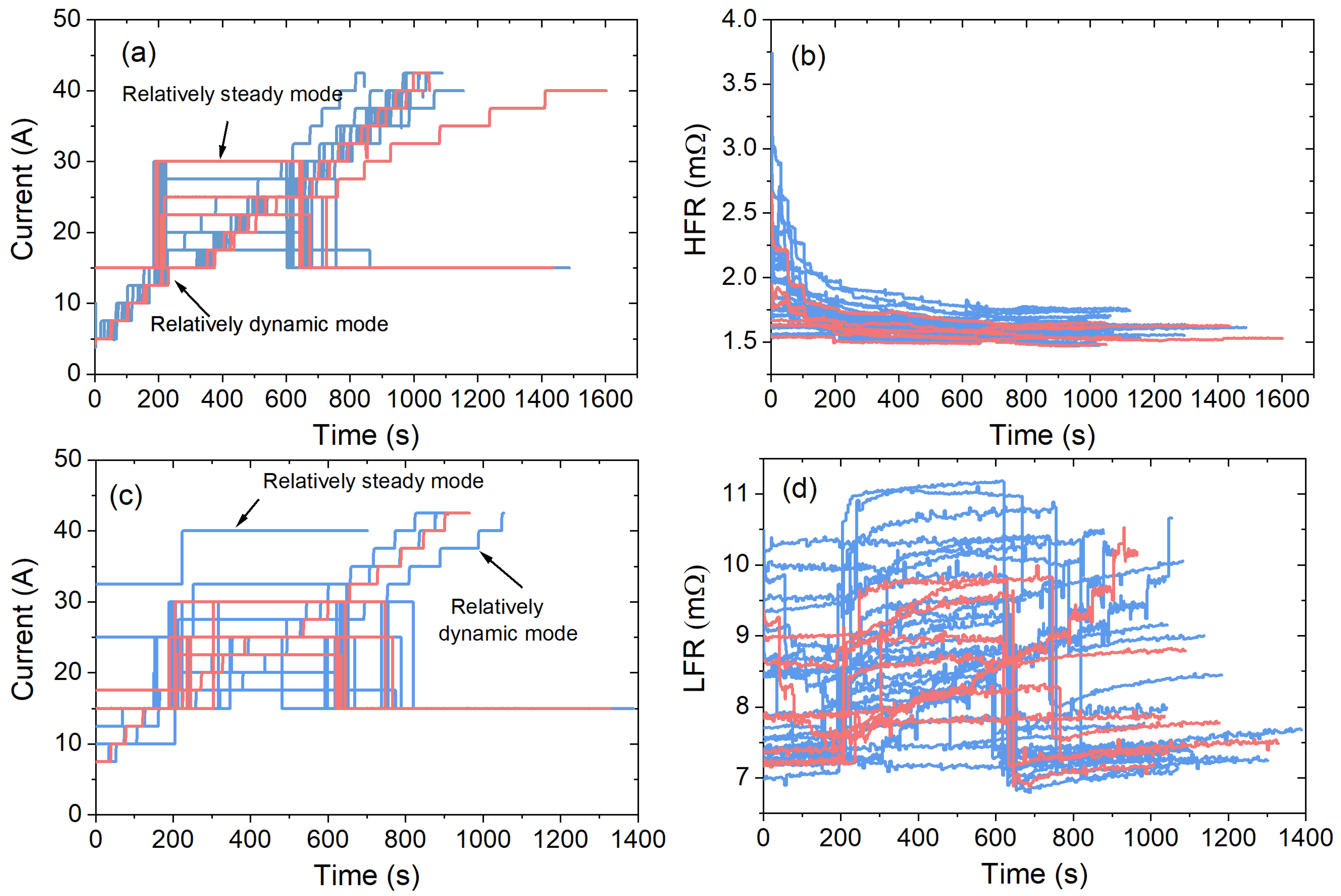
In the vehicular fuel cell system, the current is primarily determined in accordance with the power request sent by the vehicle controller, and the corresponding reactant stoichiometry, inlet pressure, and temperature requirements of the stack are determined by a look-up table. Subsequently, the objective values of these parameters are adjusted in relation to any changes in current. For example, the operating temperature and inlet pressure will increase with the current, while the air stoichiometry will typically decrease slightly due to the capacity limitation of the air compressor. Since adjusting the operating conditions of the tested PEM fuel cell based on the test bench is a slow process, so operating conditions expect the current to remain the same when running a test sequence. At the same time, the conditions of any given sequence are distinct from other operating sequences. Figure 2 illustrates corresponding characteristic frequency impedance results for given operating current settings. The HFR dataset comprises a total of 37 sequences under varying conditions, whereas the LFR dataset consists of 34 sequences in diverse conditions. A data acquisition frequency of 1 Hz was employed in order to ensure the accuracy of the recordings. Furthermore, two current modes have been deliberately designed, namely the relatively dynamic mode and the relatively steady mode. It is noteworthy that, in the relatively dynamic mode, the current changes rapidly over time and the current plateau time is short. In contrast, in the relatively steady state mode, the plateau time of the working current is extended in order to simulate the fuel cell system of a commercial vehicle in long haul. Moreover, it can be seen that the current alters rapidly during the experiment, whereas HFR and LFR are related to the equilibrium process of membrane water content and reaction concentration, reflecting the accumulation process over a much longer period. From all the measurement sequences, a randomly chosen number of sequences (marked in red) are selected for model validation, while the rest (marked in blue) are used for the training of the estimation model.

3. Impedance Estimation Framework

Having assessed the frequency of the impedance, the input signal, and the dataset, this section focuses on elucidating the preprocessing process preceding data input, the chosen model framework, and the essential details of the model implementation.

3.1. Data Processing

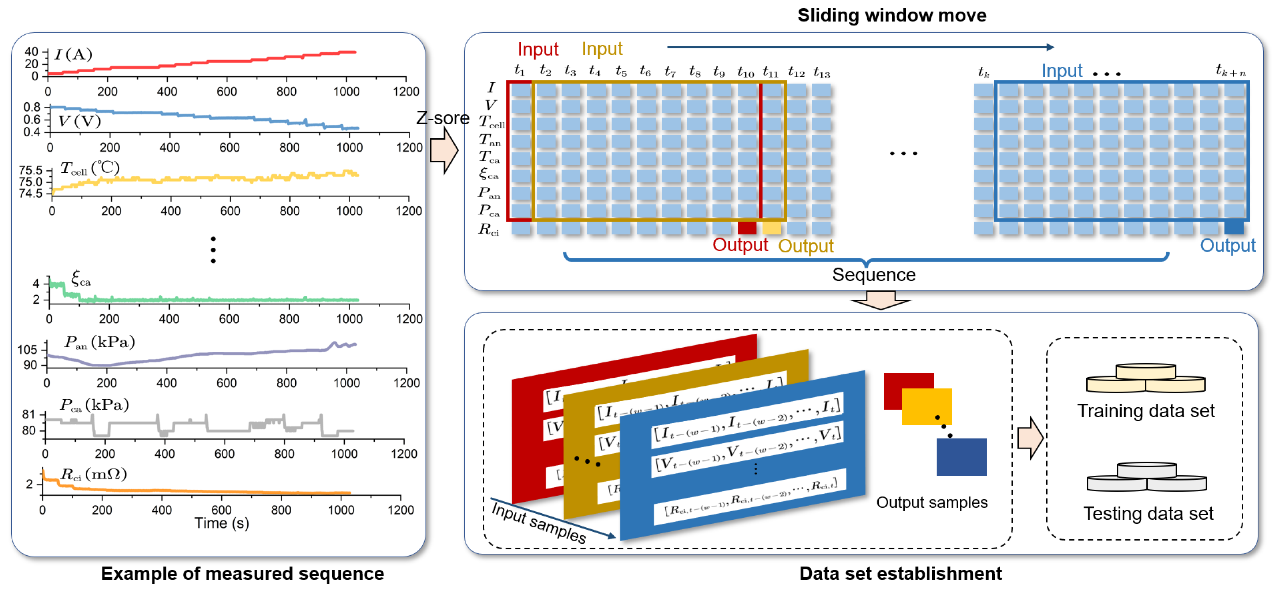
Prior to training the model, data processing is necessary in order to ensure the consistency of units and value ranges of the input signals. To facilitate the convergence of the model in the training process, the raw data is normalized using a common method of Z-score normalization. Subsequently, all the normalized input signal sequences of the predefined training and testing sequences were obtained. A sliding window was applied along with the measured sequence to cut both datasets and reorganize them as a series of limited-length two-dimensional feature maps. The specific operation of the sliding window is displayed in Figure 3, where parameter 8 × 10 × 1 represents the height, width, and channel number of the input feature map, and the width of the sliding window is set to 10 considering the appropriate size of the receptive field. In addition, the measured characteristic frequency impedance corresponding to the last moment of each sequence is used as the output. This allows the establishment of the training and testing datasets.

3.2. Model Framework

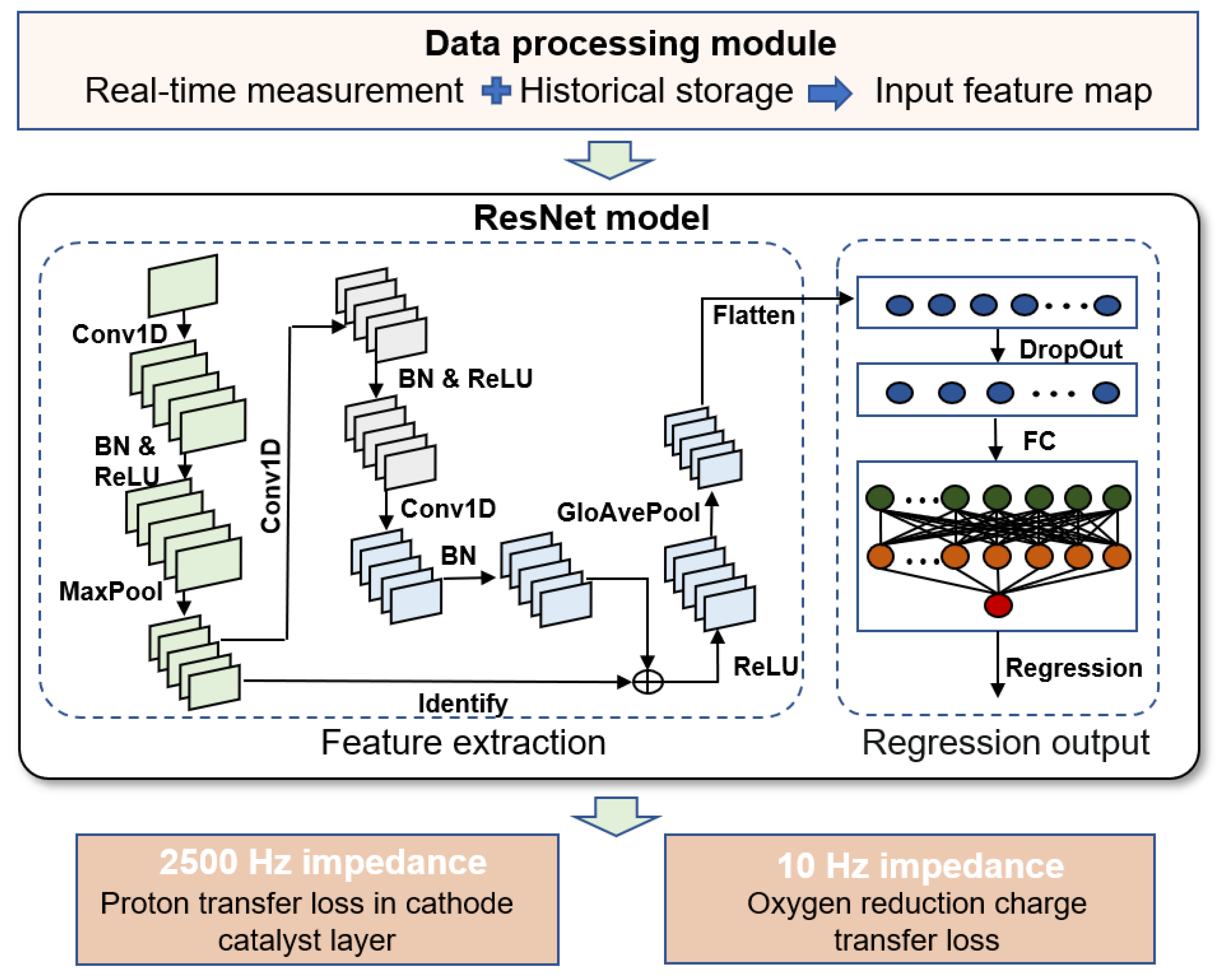
The proposed estimation framework of characteristic frequency impedance based on the residual network is illustrated in Figure 4. Initially, the signals collected by the vehicular sensor are used to form an input feature map with historical storage information, and then normalized and input into the residual network. This residual network established here comprises a multi-layer convolutional layer, batch normalization layer, activation layer, residual connection, and full connection layer. More information about ResNet can be seen in [34]. The utilization of multiple convolutional kernels and multi-layer structures in the convolutional neural network enables the automatic extraction of multi-angle and deep-level features from the original signal, thereby exhibiting improved discrimination and generalization capabilities when compared to manually implemented input features. In this paper, the convolution layers implement one-dimensional convolutional networks (Conv1D), which allows for the better extraction of local time features with fewer computations than two-dimensional convolutional operations. The general formula of the 1D convolution can be expressed as:
x j l = i = 1 n w i , j l x j l 1 + b j l
where w i , j l is the convolution kernel; b j l is the deviation from kernel; ⊗ represents the convolution operator; j is the number of kernels; l is the number of the convolution layer; and n is the channel number.
To counter the vanishing gradient issue associated with the back-propagation process, the batch normalization (BN) layer has been introduced to ensure that the activation input values fall in regions where the nonlinear function is sensitive enough to yield a relatively large gradient. The calculation procedure of the BN layer can be expressed as follows:
μ B = 1 m i = 1 m x i
σ B 2 = 1 m i = 1 m x i μ B
x ^ i = x μ B σ B 2 + ε
y i = γ x ^ i + β B N γ , β x i
where μ B and σ B 2 are the mean value and variance values, respectively; ε is the infinitesimal value; x i and y i denote the input features and output features of the BN, respectively; and m is the number of samples in the current batch.
The incorporation of the activation function serves to enable a nonlinear mapping of input data so that the model may accommodate the nonlinear relationship between input data and labels. Particularly, the ReLU function max 0 , x is adopted due to its greater stability and effectiveness with respect to gradient back propagation in neural networks. The pooling layer typically executes down-sampling operations on the feature map primarily for the integration of feature information and dimensionality reduction. The maximum pooling (MaxPool) layer and global average pooling (GloAvePool) layer are introduced. More importantly, an identity mapping, namely residual connection, is employed between the first and third convolution. Based on this, the error from the lower layer can be propagated to the upper layer via direct connection during the training process, making it possible to leverage both the objective function gradient and the residual gradient. After a series of convolutional processing, the multi-channel two-dimensional feature map is flattened and then input into the input Dropout layer, in which certain neurons are randomly disconnected with a probability, thus increasing the generalization ability of the model. Finally, it is input into three fully connected layers and the regression estimation of characteristic frequency impedance is achieved. The details of the developed ResNet are provided in Table 1.

3.3. Model Implementation

The above residual network model was established utilizing MATLAB 2022a, running on a laptop processor of 1.50 GHz and 16 GB RAM. A grid search approach was utilized to find appropriate hyperparameters, if necessary. The Adam algorithm was chosen as the training algorithm due to its high computational efficiency and low memory requirement; moreover, the parameter update was unaffected by the gradient scaling transformation. The maximum epoch was set to 80, depending on the actual convergence trend, while the minimum batch size of each training epoch was established at 2000. The dynamic learning rate was initially set to 0.001 and decreased piecewise every 5 epochs in order to prevent training loss oscillation and overfitting. After each training round, the accuracy of the current model was compared with that of the previous optimal model; if the accuracy exceeded the previous optimal model, the current model was saved. This process was repeated until the training number reached the set number of iterations. During the training process, the mean square error was selected as the loss function, with the following expression:
L o s s = 1 2 N i = 1 M y i y ^ i 2
where y ^ i is the model predicated impedance; y i is the measured impedance by the frequency response analyzer; and M is the sample number of the training dataset.

4. Results and Discussion

In this section, firstly, the trained residual network was compared with the regression models typically employed in other studies and then the robustness of the method was ascertained by applying different signal-to-noise ratio noises to the original dataset to stress the advantages of the residual network. Ultimately, the effect of various input signals on the accuracy of the impedance estimation was explored.

4.1. Accuracy Comparison of Different Models

The traditional back-propagation (BP) fully connected network, support vector regression (SVR), one-dimensional convolution neural network (CNN1d), two-dimensional convolution neural network (CNN2d), and short long-term memory (LSTM) network, were used for comparison. These models were also implemented based on MATLAB 2022a. To be specific, the BP hidden layer node was set to 128. The SVR used the Gaussian kernel function, and the hyperparameters were determined using the grid optimization method. The parameters of CNN1d were consistent with those of ResNet, which contained a three-layer convolutional structure without residual connection (kernel size: 5; channel: 128; padding; step size 1). CNN2d also had a three-layer convolution structure, but the feature graph convolution adopted a two-dimensional convolution calculation, where the convolution kernel size was 5 × 5, the convolution channel was 128, and the step size was 1. The LSTM is a three-layer stack structure, and the number of nodes was set to 128, 64, and 1, respectively.
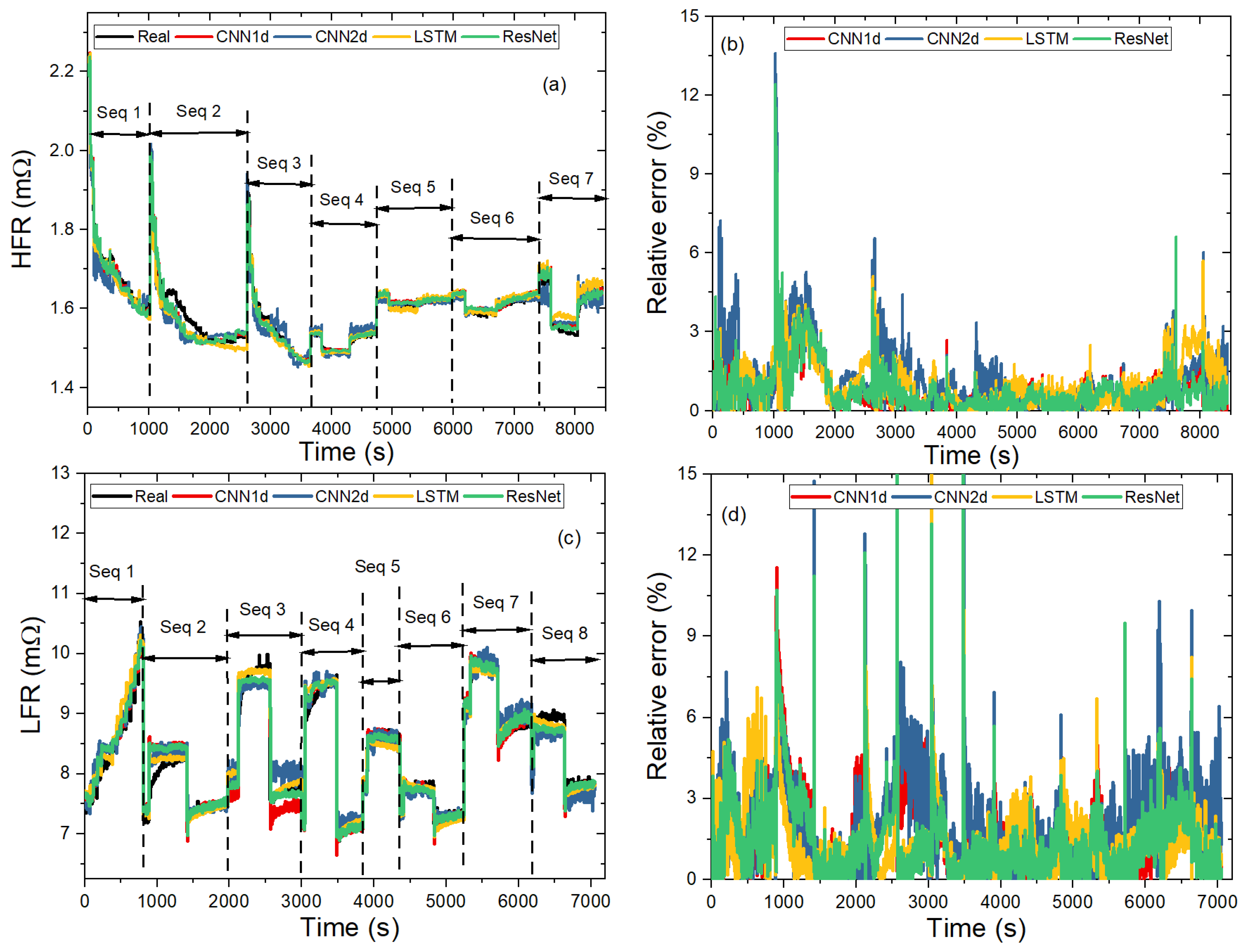
The HFR estimated results and computational time of different models are shown in Figure 5a,b and Table 2, where “Seq” represents the test sequence, and the time is recorded using tic and toc. To reflect the estimated accuracy, the relative error (RE) and mean absolute percentage error (MAPE) with the definitions of
R E = y i y ^ i y i × 100 %
M A P E = i = 1 K y i y ^ i y i × 100 %
were used, and K is the sample number of the testing dataset. Due to the significant estimation error of traditional machine learning models of BP and SVR, it is not shown in specific results to clearly display the results of deep learning models. It can be seen that all deep learning networks can accurately follow the actual value of high-frequency impedance under different test sequences, presenting a satisfactory estimation effect. In comparison, it was difficult for BP and SVR to learn the nonlinear relationship between input operating conditions and impedance with higher relative error. In addition, their training time was about 61 min and 82 min, respectively. In terms of deep learning models, large errors mainly appeared in the small current density interval of test sequence 2 because the air stoichiometry of this test sequence was 1.5, while the air stoichiometry of most training sequences in the training dataset was set to 2.0, resulting in incomplete learning of the model under low air stoichiometry. Additionally, CNN1d was found to have higher accuracy and shorter training time compared to CNN2d, suggesting its suitability for time series-related tasks. The introduction of the residual connection to the ResNet model has resulted in a 0.802% MAPE, which is 2.53% lower than that of CNN1d. With these in mind, the residual connection was found to significantly accelerate network learning and convergence while reducing the training and testing time by 29.85% and 5.34%, respectively. When compared to the LSTM employed in the preceding paper, ResNet demonstrated an impressive 23.02% decrease in the MAPE, albeit with slightly greater computational time. Consequently, the ResNet model proposed here can provide high-precision HFR estimates with reasonable computational expenditure, hence making it suitable for determining the internal membrane water content in fuel cells.
The LFR estimated results of different models are presented in Figure 5c,d and Table 2. Specific BP and SVR estimation results are not provided. As can be observed, despite the relatively large errors that appeared when the load transient changed in sequences 2 to 4, all the deep learning models could still accurately track the actual measurements of low-frequency impedance, as supported by the relative error of less than 3%. Among the models, CNN1d was found to be more accurate and computationally efficient than CNN2d. Notably, the accuracy of LSTM estimation was higher than that of CNN1d, with a reduction of 14.40% in MAPE. Furthermore, the MAPE of ResNet was found to be 1.386%, which was facilitated by 4.11% compared with LSTM. These results indicate that the proposed ResNet also has higher estimation accuracy in low-frequency impedance estimation.

4.2. Model Robustness against Different Noise Levels

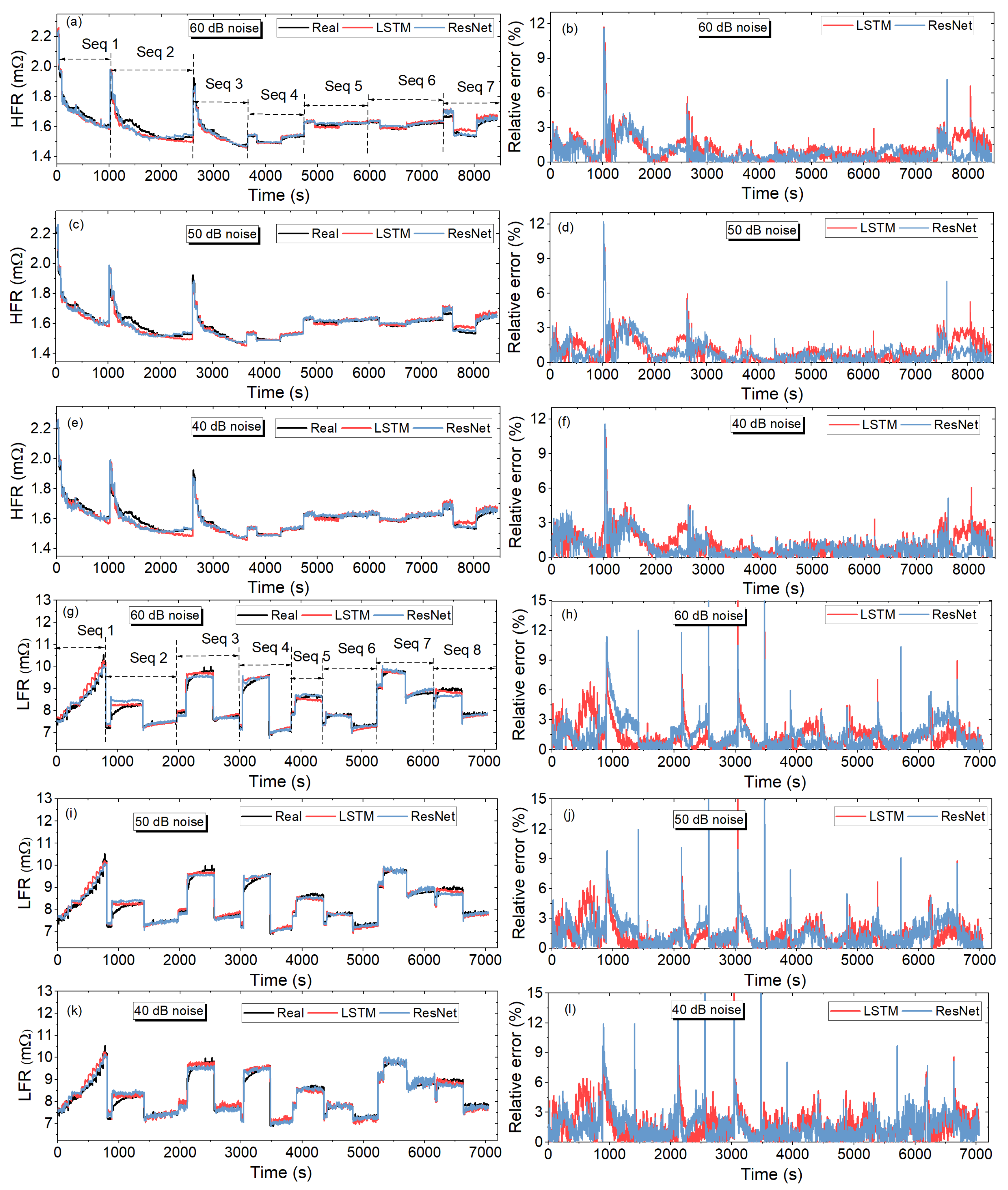
Unlike the laboratory test bench, fuel cell systems contain high-voltage components, such as air compressors, hydrogen cycle pumps, water pumps, and DC/DC converters, which may affect the acquisition of model input signals due to electromagnetic compatibility effects. To this end, Gaussian white noise of signal-to-noise ratios of 60 dB, 50 dB, and 40 dB were added to the original dataset, and the model was then retrained and tested. As LSTM and ResNet exhibited superior performance in the precision comparison, robustness tests under noise interference were conducted on these two models only. The detailed estimated results and relative errors are depicted in Figure 6. It can be seen that, despite the presence of noise in the original input signals, the estimation of HFR and LFR by both LSTM and ResNet still closely followed their measured values with an acceptable degree of accuracy. Specifically, even with a 40 dB noise on the input signal, the mean relative error of HFR and LFR was 0.911% and 1.610%, respectively, based on ResNet, which was 19.29% and 2.03% lower than that of LSTM, indicating that ResNet has better robustness to measured uncertainties.

4.3. The Effect of Input Signal on Model Accuracy

Taking into account the potential for sensor failure during the operation of the fuel cell system, the impact of different input conditions on the model accuracy needs to be explored. For this purpose, a new dataset was constructed using a sliding window to train and test the model after removing the specific input condition. The MAPE and decline rate of accuracy, excluding the corresponding input signal, are presented in Table 3 and Figure 7. The results demonstrate that the estimated accuracy of both LSTM and ResNet decreases after the elimination of the specific input condition; however, the MAPE of ResNet is still smaller, showing advances in the estimation of characteristic frequency impedance. Moreover, the three input conditions that notably influence the HFR estimation of ResNet are air stoichiometry, output voltage, and working current. Out of these, air stoichiometry directly affects the moisture taken away by convection in the cathode channel, with a MAPE growth rate exceeding 100%. Output voltage directly reflects the current performance of fuel cells and, thus, the removal of this input signal has a considerable impact on the estimation results, with a MAPE growth rate of 90%. Working current, on the other hand, directly decides the water content generated by the reaction and, therefore, has an impressive effect on the estimation of high-frequency impedance, with a MAPE growth rate of 72.03%. Similarly, for the LFR dataset, ResNet’s calculation accuracy remains higher than that of LSTM after removing the specific input signal, wherein output voltage, working current, and cathode inlet temperature had a remarkable effect. Voltage and current reflect the electrochemical reaction rate, thus directly determining the charge transfer loss and influencing the LFR estimation. The cathode intake temperature can reflect the relative humidity of the air on the test bench and the electrochemical reaction rate is also closely related to the hydration state of the catalyst ionomer, thereby having a profound impact on the estimation of LFR.

4.4. Discussion

The results of the proposed ResNet-based method demonstrate its effectiveness in real-time frequency-impedance estimation, providing a novel technology for impedance acquisition of the vehicle fuel cell system. In doing so, the internal state of the fuel cell can be identified via the estimated impedance to optimize its control. For instance, the estimated characteristic frequency impedance can be applied to diagnose fuel cell membrane drying, flooding, and air starvation faults through the establishment of appropriate thresholds or diagnostic models. Furthermore, the estimated HFR can be used to assess the membrane water content during the fuel cell outage purge, thereby enabling control of the purge flow and duration. Additionally, the estimated low-frequency impedance can be utilized for feedback control of concentration polarization degree during the cold start of the fuel cell system, ensuring that the fuel cell generates much heat while avoiding its deep concentration-induced irreversible attenuation. As the number of commercially available fuel cell vehicles increases, an abundance of vehicular data will be collected, providing the opportunity to capitalize on the potential of artificial intelligence algorithms and cloud-based platforms for fuel cell system management to achieve accurate state perception and prediction (see Figure 8). This can then be used to enable proactive management optimization. Furthermore, the use of data-driven methods can facilitate the development of material and structure designs based on digital twin models combined with intelligent optimal algorithms, such as genetic algorithms and particle swarm optimization, thus allowing for the optimization of fuel cell geometric and material parameters to achieve high performance.
The data-driven method presents certain limitations, such as a lack of evaluation under complex dynamic processes, which may lead to impedance estimation difficulties. In this regard, physics modeling that allows for the data-driven approach to be interpreted and for fewer data to be collected is worth exploring. Moreover, the model output depends on the quality of the datasets created. Data quality thus becomes even more significant than deep learning algorithms. To be more effective, the original data should include representative conditions of the vehicular fuel cell as much as possible. In this paper, the dataset was not comprehensive, failing to consider actual vehicle operating conditions (start-up, idling, variable load, shutdown) and the effect of low temperatures. Greater emphasis should be placed on the production of datasets, particularly for high-power stacks.

5. Conclusions

In this paper, a deep learning approach based on ResNet is presented for the estimation of the characteristic frequency impedance of the PEM fuel cell. The proposed model is capable of utilizing both previous and current information obtained from vehicular sensor data for a real-time prediction of HFR and LFR, where 2500 Hz impedance characterizing proton transfer loss and 10 Hz impedance depicting charge transfer loss are selected. The proposed scheme is validated and compared to other frequently used regression and deep learning models under a series of test sequences with different noise levels and input signals. The main conclusions are as follows: (1) The ResNet can achieve a high estimation accuracy for HFR and LFR under different test sequences. It has an overall mean absolute percentage error (MAPE) of 0.802% and 1.386%, respectively, which outperforms other regression and deep learning models. Specifically, ResNet was found to decrease the MAPE for HFR and LFR estimation by 23.02% and 4.11%, respectively, when compared to LSTM. (2) Despite the introduction of an additional 40 decibels of noise to the original signals, ResNet was still able to achieve accurate estimation for HFR and LFR, with MAPE of 0.911% and 1.610%, respectively, representing a 19.29% and 2.03% decrease in error rate compared to LSTM, thereby indicating that ResNet has greater robustness to measured uncertainties. (3) All input signals have an effect on impedance estimation. For HFR estimation, air stoichiometry, output voltage, and working current are the significantly influenced input signals, while, for LFR estimation, the effect of output voltage, working current, and cathode inlet temperature is remarkable.
To further enhance the performance of the proposed model, future research should focus on enriching the dataset through experiments more in line with vehicle operating conditions and environment, as well as developing more advanced algorithms such as combining the feature extraction capability of convolutional networks with the time series processing capability of recurrent neural networks. Additionally, intelligent optimization algorithms can be employed to optimize the hyperparameters of the model for optimum estimation performance. Moreover, the current model is based on an offline experimental dataset for model training and validation, which is still in the preliminary computer verification stage. For further validation, it is imperative to integrate the model with the controller or cloud platform of an actual vehicle fuel cell system in the future.

Author Contributions

Conceptualization, J.X. and H.Y. Methodology, J.X. Software, C.W. Validation, Y.W. Writing—original draft preparation, J.X. and H.Y. Writing—review and editing, J.X., H.Y., X.W. and H.D. Resources, C.W., X.W. and H.D. All authors have read and agreed to the published version of the manuscript.

Funding

This work was supported by the Program of Shanghai Academic/Technology Research Leader (22XD1423800).

Data Availability Statement

Data available on request from the authors.

Conflicts of Interest

The authors declare no conflict of interest.

References

  1. Su, D.; Zheng, J.; Ma, J.; Dong, Z.; Chen, Z.; Qin, Y. Application of Machine Learning in Fuel Cell Research. Energies 2023, 16, 4390. [Google Scholar] [CrossRef]
  2. Reithuber, P.; Poimer, F.; Brandstätter, S.; Schutting, E.; Buchberger, S.; Trattner, A.; Eichlseder, H. Experimental Investigation of the Influence of NO on a PEM Fuel Cell System and Voltage Recovery Strategies. Energies 2023, 16, 3720. [Google Scholar] [CrossRef]
  3. Jiao, J.; Chen, F. Humidity estimation of vehicle proton exchange membrane fuel cell under variable operating temperature based on adaptive sliding mode observation. Appl. Energy 2022, 313, 118779. [Google Scholar] [CrossRef]
  4. Yuan, H.; Dai, H.; Wei, X.; Ming, P. Internal polarization process revelation of electrochemical impedance spectroscopy of proton exchange membrane fuel cell by an impedance dimension model and distribution of relaxation times. Chem. Eng. J. 2021, 418, 129358. [Google Scholar] [CrossRef]
  5. Yuan, H.; Tan, D.; Wei, X.; Dai, H. Fault Diagnosis of Fuel Cells by a Hybrid Deep Learning Network Fusing Characteristic Impedance. IEEE Trans. Transp. Electrif. 2023. [Google Scholar] [CrossRef]
  6. Lin, R.; Liu, D.; Xia, S.; Ma, T.; Dutruel, B. Stack shut-down strategy optimisation of proton exchange membrane fuel cell with the segment stack technology. Int. J. Hydrogen Energy 2020, 45, 1030–1044. [Google Scholar] [CrossRef]
  7. Choi, H.; Kim, J.; Kwon, O.; Yoo, H.; Kim, H.; Cha, H.; Park, T. Observation of flooding-induced performance enhancement in PEMFCs. Int. J. Hydrogen Energy 2022, 47, 6259–6268. [Google Scholar] [CrossRef]
  8. Moçotéguy, P.; Ludwig, B.; Beretta, D.; Pedersen, T. Study of the impact of reactants utilization on the performance of PEMFC commercial stacks by impedance spectroscopy. Int. J. Hydrogen Energy 2021, 46, 7475–7488. [Google Scholar] [CrossRef]
  9. Jeppesen, C.; Araya, S.S.; Sahlin, S.L.; Andreasen, S.J.; Kær, S.K. An EIS alternative for impedance measurement of a high temperature PEM fuel cell stack based on current pulse injection. Int. J. Hydrogen Energy 2017, 42, 15851–15860. [Google Scholar] [CrossRef] [Green Version]
  10. Ritzberger, D.; Striednig, M.; Simon, C.; Hametner, C.; Jakubek, S. Online estimation of the electrochemical impedance of polymer electrolyte membrane fuel cells using broad-band current excitation. J. Power Sources 2018, 405, 150–161. [Google Scholar] [CrossRef]
  11. Yuan, H.; Dai, H.; Ming, P.; Li, S.; Wei, X. A new insight into the effects of agglomerate parameters on internal dynamics of proton exchange membrane fuel cell by an advanced impedance dimension model. Energy 2022, 253, 124202. [Google Scholar] [CrossRef]
  12. Bullecks, B.; Suresh, R.; Rengaswamy, R. Rapid impedance measurement using chirp signals for electrochemical system analysis. Comput. Chem. Eng. 2017, 106, 421–436. [Google Scholar] [CrossRef]
  13. Lu, H.; Chen, J.; Yan, C.; Liu, H. On-line fault diagnosis for proton exchange membrane fuel cells based on a fast electrochemical impedance spectroscopy measurement. J. Power Sources 2019, 430, 233–243. [Google Scholar]
  14. Debenjak, A.; Boškoski, P.; Musizza, B.; Petrovčič, J.; Juričić, D. Fast measurement of proton exchange membrane fuel cell impedance based on pseudo-random binary sequence perturbation signals and continuous wavelet transform. J. Power Sources 2014, 254, 112–118. [Google Scholar] [CrossRef]
  15. Du, R.; Wang, X.; Dai, H.; Wei, X.; Ming, P. Online impedance spectrum measurement of fuel cells based on Morlet wavelet transform. Int. J. Hydrogen Energy 2021, 46, 24339–24352. [Google Scholar] [CrossRef]
  16. Yuan, H.; Du, R.; Wang, X.; Wei, X.; Dai, H. Advanced Online Broadband Impedance Spectrum Acquisition of Fuel Cells by S-Transform. IEEE Trans. Ind. Electron. 2023, 70, 3740–3750. [Google Scholar] [CrossRef]
  17. Heinzmann, M.; Weber, A.; Ivers-Tiffée, E. Advanced impedance study of polymer electrolyte membrane single cells by means of distribution of relaxation times. J. Power Sources 2018, 402, 24–33. [Google Scholar] [CrossRef]
  18. Ren, P.; Pei, P.; Li, Y.; Wu, Z.; Chen, D.; Huang, S.; Jia, X. Diagnosis of water failures in proton exchange membrane fuel cell with zero-phase ohmic resistance and fixed-low-frequency impedance. Appl. Energy 2019, 239, 785–792. [Google Scholar]
  19. Meyer, Q.; Liu, S.; Ching, K.; Da Wang, Y.; Zhao, C. Operando monitoring of the evolution of triple-phase boundaries in proton exchange membrane fuel cells. J. Power Sources 2023, 557, 232539. [Google Scholar]
  20. Xu, X.; Li, K.; Liao, Z.; Cao, J.; Wang, R. A Closed-Loop Water Management Methodology for PEM Fuel Cell System Based on Impedance Information Feedback. Energies 2022, 15, 7561. [Google Scholar] [CrossRef]
  21. Jiang, P.; Chen, J.; Jin, L.; Kumar, L. Adaptive Condition Monitoring for Fuel Cells Based on Fast EIS and Two-Frequency Impedance Measurements. IEEE Trans. Ind. Electron. 2023, 70, 8517–8525. [Google Scholar]
  22. Choi, H.; Jang, H.; Kim, J.; Kwon, O.; Yoo, H.; Cha, H.; Jeong, S.; So, Y.; Park, T. Real-time detection of flooding in polymer electrolyte membrane fuel cells using high-frequency electrochemical impedance. J. Power Sources 2023, 580, 233311. [Google Scholar]
  23. Wang, H.; Gaillard, A.; Hissel, D. A review of DC/DC converter-based electrochemical impedance spectroscopy for fuel cell electric vehicles. Renew. Energy 2019, 141, 124–138. [Google Scholar] [CrossRef]
  24. Tian, J.; Xiong, R.; Chen, C.; Wang, C.; Shen, W.; Sun, F. Simultaneous prediction of impedance spectra and state for lithium-ion batteries from short-term pulses. Electrochim. Acta 2023, 449, 142218. [Google Scholar]
  25. Guo, J.; Che, Y.; Pedersen, K.; Stroe, D.I. Battery impedance spectrum prediction from partial charging voltage curve by machine learning. J. Energy Chem. 2023, 79, 211–221. [Google Scholar]
  26. Ma, T.; Zhang, Z.; Lin, W.; Cong, M.; Yang, Y. Impedance prediction model based on convolutional neural networks methodology for proton exchange membrane fuel cell. Int. J. Hydrogen Energy 2021, 46, 18534–18545. [Google Scholar] [CrossRef]
  27. Lin, T.; Hu, L.; Wisely, W.; Gu, X.; Cai, J.; Litster, S.; Kara, L.B. Prediction of high frequency resistance in polymer electrolyte membrane fuel cells using long short term memory based model. Energy AI 2021, 3, 100045. [Google Scholar]
  28. Yuan, H.; Dai, H.; Ming, P.; Wang, X.; Wei, X. Quantitative analysis of internal polarization dynamics for polymer electrolyte membrane fuel cell by distribution of relaxation times of impedance. Appl. Energy 2021, 303, 117640. [Google Scholar]
  29. Yuan, H.; Dai, H.; Ming, P.; Zhao, L.; Tang, W.; Wei, X. Understanding dynamic behavior of proton exchange membrane fuel cell in the view of internal dynamics based on impedance. Chem. Eng. J. 2022, 431, 134035. [Google Scholar] [CrossRef]
  30. Lee, J.; Salihi, H.; Lee, J.; Ju, H. Impedance modeling for polymer electrolyte membrane fuel cells by combining the transient two-phase fuel cell and equivalent electric circuit models. Energy 2022, 239, 122294. [Google Scholar]
  31. Liu, X.; Peng, F.; Lou, G.; Wen, Z. Liquid water transport characteristics of porous diffusion media in polymer electrolyte membrane fuel cells: A review. J. Power Sources 2015, 299, 85–96. [Google Scholar] [CrossRef]
  32. Xing, L.; Das, P.K.; Song, X.; Mamlouk, M.; Scott, K. Numerical analysis of the optimum membrane/ionomer water content of PEMFCs: The interaction of Nafion® ionomer content and cathode relative humidity. Appl. Energy 2015, 138, 242–257. [Google Scholar]
  33. Yuan, H.; Dai, H.; Ming, P.; Zhan, J.; Wang, X.; Wei, X. A fuzzy extend state observer-based cascade decoupling controller of air supply for vehicular fuel cell system. Energy Convers. Manag. 2021, 236, 114080. [Google Scholar] [CrossRef]
  34. He, K.; Zhang, X.; Ren, S.; Sun, J. Deep Residual Learning for Image Recognition. In Proceedings of the 2016 IEEE Conference on Computer Vision and Pattern Recognition (CVPR), Las Vegas, NV, USA, 27–30 June 2016; pp. 770–778. [Google Scholar]
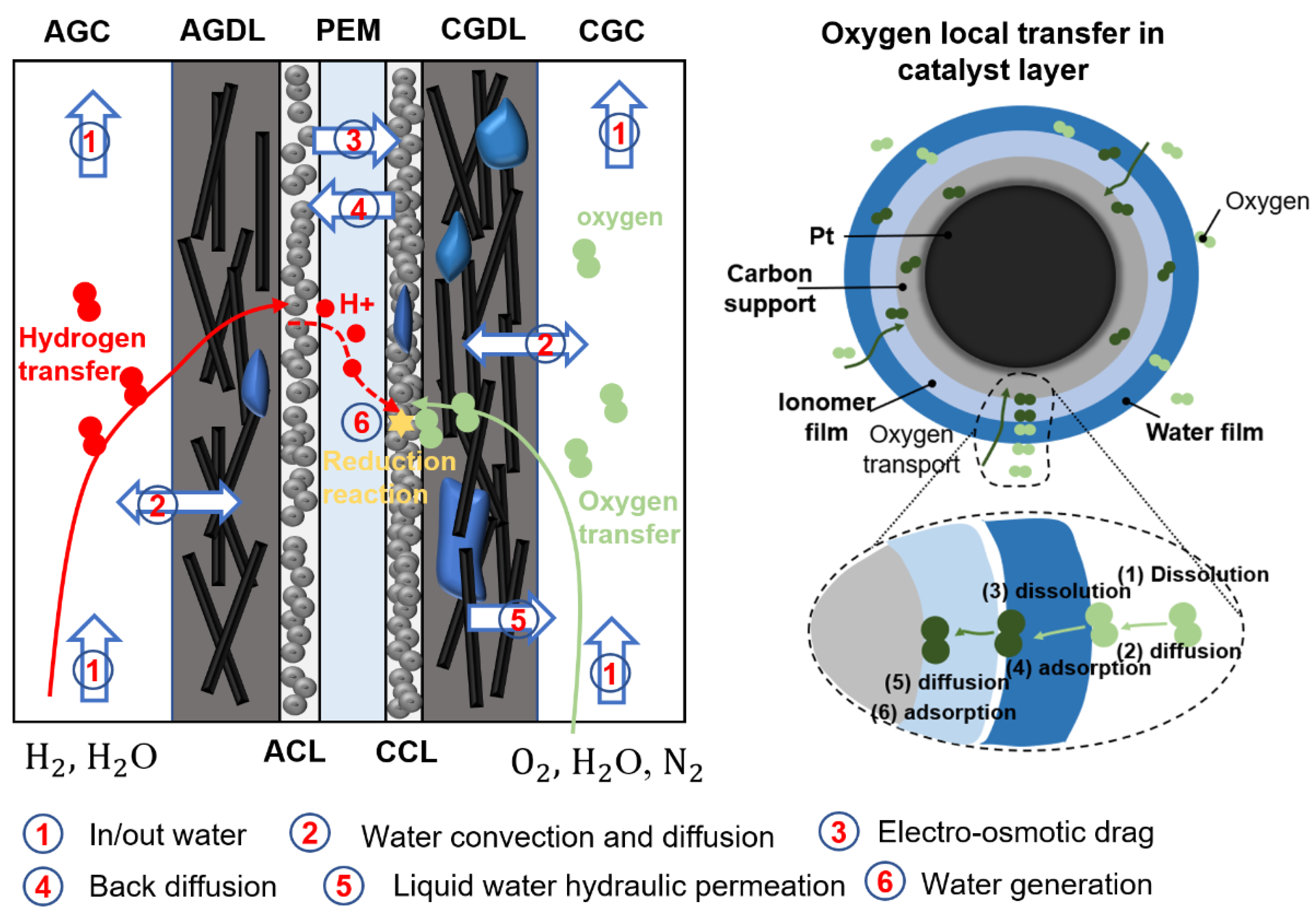
Figure 1. The water and oxygen transfer processes inside the PEM fuel cell.
Energies 16 05556 g001
Figure 2. Measured dataset for characteristic frequency impedance: (a) current and (b) corresponding HFR; (c) current and (d) corresponding LFR. The blue and red curves represent sequences in the training and testing set, respectively.
Energies 16 05556 g002
Figure 3. The process of data reconstruction using a sliding window.
Energies 16 05556 g003
Figure 4. The basic architecture of residual network model for characteristic frequency impedance estimation.
Energies 16 05556 g004
Figure 5. (a) The specific estimated results and (b) relative error for HFR; (c) the specific estimated results and (d) relative error for LFR.
Energies 16 05556 g005
Figure 6. The specific estimated results and relative error for HFR, (a,b) 60 dB, (c,d) 50 dB, (e,f) 40 dB; the specific estimated results and relative error for LFR, (g,h) 60 dB, (i,j) 50 dB, (k,l) 40 dB.
Energies 16 05556 g006
Figure 7. The increase rate in MAPE of the model after removing certain input signals for (a) HFR dataset and (b) LFR dataset.
Energies 16 05556 g007
Figure 8. The application of data technology for fuel cell system management and design.
Energies 16 05556 g008
Table 1. Configuration of the developed ResNet.
OrderDetailed Information
1Convolution layer (Kernel size: 5; Channel: 128; Padding; Step size 1)
2Batch normalization layer
3ReLU activation layer
4Maximum pooling (residual connection is performed with order 9)
5Convolution layer (Kernel size: 5; Channel: 128; Padding; Step size 1)
6Batch normalization layer
7ReLU activation layer
8Convolution layer (Kernel size: 5; Channel: 128; Padding; Step size 1)
9Batch normalization layer (residual connection is performed with order 4)
10ReLU activation layer
11Global average pooling layer
12Flatten layer
13Dropout layer (probability: 0.05)
14Fully connected layer (Dense: 128)
15Fully connected layer (Dense: 64)
16Fully connected layer (Dense: 1)
Table 2. Comparison for the estimation results and computational time.
ModelHFR Data SetLFR Data Set
Training TimeTesting TimeMAPETraining TimeTesting TimeMAPE
BP3709 s0.121 s6.984%2895 s0.200 s5.616%
SVR4970 s1.726 s4.811%1818 s0.983 s4.759%
CNN1d536 s6.478 s0.823%379 s5.126 s1.689%
CNN2d2404 s5.937 s1.193%1637 s4.934 s2.071%
LSTM288 s3.600 s1.042%161 s2.411 s1.446%
ResNet376 s6.132 s0.802%238 s4.822 s1.386%
Table 3. MAPE of LSTM and ResNet by removing specific signals.
Excluded SignalHFR Data SetLFR Data Set
LSTMResNetLSTMResNet
I1.642%1.380%2.026%1.797%
V1.573%1.545%2.862%2.299%
T cell 1.093%1.077%1.464%1.510%
T an 1.074%1.033%1.464%1.445%
T ca 1.183%1.101%2.393%1.741%
ξ ca 2.065%1.994%1.481%1.438%
P an 1.055%1.037%1.447%1.423%
P ca 1.065%1.018%1.508%1.430%
Disclaimer/Publisher’s Note: The statements, opinions and data contained in all publications are solely those of the individual author(s) and contributor(s) and not of MDPI and/or the editor(s). MDPI and/or the editor(s) disclaim responsibility for any injury to people or property resulting from any ideas, methods, instructions or products referred to in the content.