Abstract
Neural network approaches have commonly been used to solve complex mathematical equations in the literature. They have inspired the modifications of state controllers and are often implemented for electrical drives with an elastic connection. Given that the addition of a virtual signal can provide adaptive properties to classical controllers and that selected feedback signals can also be replaced with a virtual state variable from a neural network, several combinations can be considered and compared. In this paper, Radial Basis Function neural-network-based control algorithms are proposed in which online updating of the output weights is used. Analyses of simulation experiment results reveal that the proposed control algorithms significantly improve the operation of classic-state feedback controllers applied to two-mass systems in the presence of parameter uncertainty.
1. Introduction
The prevalence of electrical drives can be observed throughout industrial applications and home appliances. They are a viable choice when high precision of speed or position control is required [1]. Additionally, with current advance in electrical drives and digital signal processing, many state-of-the-art solutions can be easily implemented [2]. However, sometimes control accuracy may be affected by the mechanical structure of the device. Because of torsion, the speed of the motor does not directly transfer to the speed of the load machine [3]. Rolling mills [4], wind turbines [5], robotic manipulators [6,7,8,9], exoskeletons [10,11], electric cars [12], and countless similar mechanisms are all affected by this phenomenon, making it a crucial scientific problem to be solved.
Applications with a complex mechanical structure are affected by multiple disturbances. An increased number of elements increases the influence of friction, backlash, and other non-linearities [13]. Torsion applied to the shaft may introduce oscillations of state variables (angular speed of the motor and load machine and torsional torque), which significantly hinders the system’s control precision [14]. With heavier loads and the likelihood of an external load torque being applied, mechanical forces may cause rupture or other irreparable damage to structural components [15]. Additionally, with the limited possibility to control the speed of the motor, stability issues might occur [16].
Available methods for mitigating the effects of elastic connections can be divided into two main categories: mechanical and software solutions. Mechanical methods are focused on introducing additional elements to the structure of the drive [17]. Even though physical dampeners might appear as a promising solution, they have multiple drawbacks: they significantly increase the cost of the drive; the structure becomes even more complex; and with more elements and connections, there are more possibilities for the mechanism to malfunction (reduced reliability of the drive). One way to non-invasively reduce the impact of torsion is to implement a reference signal filter [18]. With a deliberate choice of signal limiting, the effect of torsion can be minimized. On the other hand, introducing a ramp may significantly hinder the operation of the drive in dynamic states.
The most-often selected solution for electric motor control is the PI (Proportional-Integral) control strategy [19,20,21]. The choice is motivated by the ease of practical implementation in programmable devices (such as digital signal processors and microcontrollers) and low complexity, which results in fast calculation and low memory usage. They provide satisfactory results in controlled environments with little to no change in operating conditions. In its basic form, however, this method does not take any information about the state of the load machine, making it unsuitable for applications with elastic mechanical connections [22]. To improve the performance of the structure, additional feedback from state variables can be supplied. This solution may form a PI control structure with a combination of feedback signals [23] or may be transformed into an integral state feedback controller [24,25,26]. These two solutions significantly improve the operation of the drive by suppressing the oscillations of speed and torque and limiting the occurrence of overshoots. Unfortunately, these two solutions suffer from one drawback: their sensitivity to parameter uncertainty [27]. Their gains are calculated and set once according to the identified parameters of the plant. In applications wherein the parameters of the structure may vary during their operation (e.g., change of the inertia of the load machine), constant gains do not provide any flexibility to match the needed control precision. Therefore, to tackle this issue, adaptive control structures can be considered.
The previously mentioned algorithms work under the assumption that the initial state of the plant is fully known and that its parameters do not change over time. In many industrial applications, this is not the case; therefore, for more-precise results, adaptive structures are applied. Model Reference Adaptive Systems (MRAS) are often implemented to achieve adaptive properties [28]. Their principle of operation is based on comparison between the desired operation from a reference model and the actual output of the plant. The difference between those signals is fed to an adaptation algorithm, which changes the parameters of the controller. With the gains being constantly adjusted to match the current state of the system, better results can be expected. Other strategies focus on predicting future states of the machine, which improves the calculation of the control signal for the plant. Such solutions are commonly referred to as Model Predictive Control (MPC) [29]. Those methods provide excellent results. However, they are computationally heavy and often depend on accurate estimation of load torque. Load torque must be treated as an external disturbance; therefore, establishing a tool to precisely assess its value at all times is a very difficult task [30]. Intelligent structures with neural networks are widely investigated in the modern literature [31,32,33,34,35]. Neural networks can be utilized in electric drives for multiple purposes, such as state variable estimation [36], motor condition monitoring and diagnosis [37], enabling control with damaged sensors (often referred to as Fault-Tolerant Control) [38], and adaptive control [39]. To achieve adaptive qualities, training of the network must be performed online, i.e., during the operation of the drive. Other significant aspects of designing neural control algorithms focus on the topology of the network. The number of hidden layers, number of neurons in each layer, possible recurrent connections, and activation functions all have to be predefined.
Radial Basis Function Neural Networks (RBFNNs) are widely known and used in tasks of interpolation and function approximation [40,41]. Their output can be interpreted as an expansion of a desired function into a series of radial basis functions (usually Gaussian functions), the centers of which are distributed across the input space. What speaks in favor of implementing RBFNNs over other interpolation methods is their differentiability [42], which allows gradient methods to be used for training, and their easy parametrization, which allows optimization algorithms to be used to better distribute the centers and widths of RBFs [43].
Electric drives with flexible joints, uncertain dynamics, and non-linear phenomena demand a control algorithm that takes all these features into account. With good ability to find solutions to nonlinear and partial-derivative equations, RBFNNs are a good candidate tool to improve known control algorithms by providing adaptive qualities to match the current state of the drive. The use of this structure should mitigate the effect of the undesirable circumstances that affect the operation of the mechanic structure.
Our previous considerations of the topic of neural control of electric drives with elastic connections focused on the possible use of RBFNNs in combination with classic PI control scheme. The results are summarized in [44]. Even though the structure showed adaptive properties and the overshoots resulting from parameter uncertainty were mitigated, the lack of information about the state of the load machine had a crucial effect on the obtained results. This research is the continuation of our previous studies. This time, our goal is to verify the possible use of RBFNNs with a commonly used control structure that incorporates signals from other state variables (including the state of the load machine). State Feedback Control has been selected, and the neural structure has been implemented in two scenarios: as a virtual generator of an additional signal and as a replacement of the signal from torsional torque.
In this article, the possible use of adaptive RBFNN state feedback controllers is investigated. The combination of a stable control structure with an adaptive element can provide a solution to two-mass system control that withstands parameter uncertainty. First, a mathematical description of the plant, the State Feedback Controller (SFC), the RBFNN, and the training method is given. Then, simulation studies of the proposed control algorithms are presented. The following section shows the experimental verification of the numerical tests. The test bench is composed of two 0.5 kW DC motors connected with a long, steel shaft. The control algorithms are implemented on a dSPACE DS1103 fast-prototyping board. Lastly, the results are briefly summarized and discussed.
2. Adaptive Control Structure with Virtual Signal Generator Applied for Two-Mass System
2.1. Mathematical Description of the Object and the SFC
The analyzed plant is commonly represented as two conjoined masses. The mechanical connection is established through an elastic shaft. In the literature, such a structure is often referred to as a two-mass system. Its behavior can be described with a system of differential equations [45]:
where and are the angular speeds of the motor and the load machine, respectively; , , and are the electromagnetic, torsional and load torques, respectively; , , and are the time constants of the mechanical components of the structure: the motor, load, and shaft, respectively.
A simplified visual representation of a two-mass system is shown in Figure 1.

Figure 1.
Simplified model of a two-mass system.
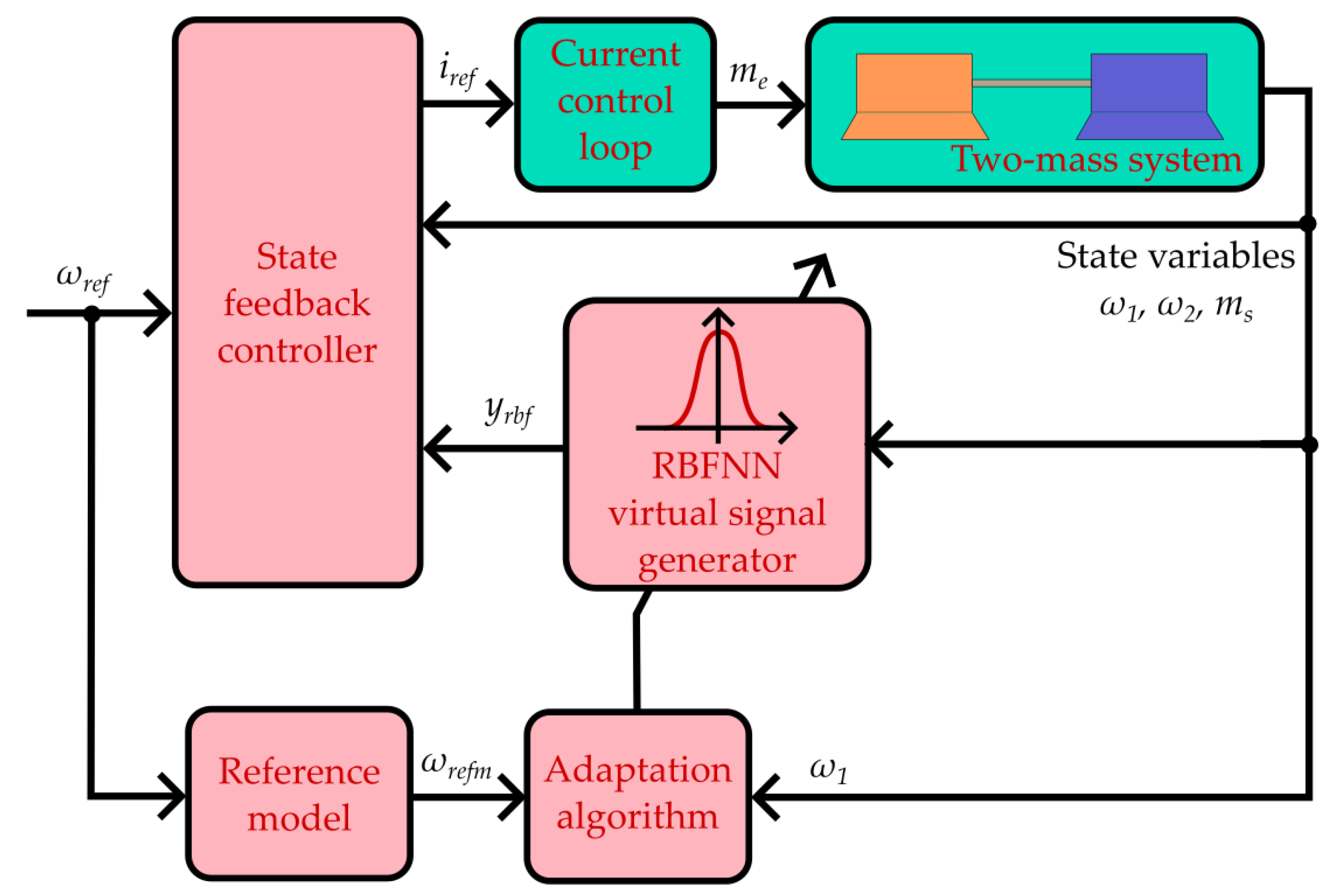
As previously discussed, PI cascade control might not provide satisfactory results for speed control. To enhance the performance of the control structure, additional feedback signals from state variables can be introduced. Examples in the literature show that state feedback control is a far-more-effective solution [46]. The cascade control scheme can be divided into sub-elements: the controlled plant, the inner torque/current control loop, and the outer speed control loop that includes feedback from the additional state variables. The idea is visually presented in Figure 2.
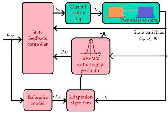
Figure 2.
General idea of the proposed State Feedback Control Algorithm.
The inner control loop consists of the electromagnetic part of the motor, power electronics, measuring devices, signal conditioners, analog-to-digital converter, and the current controller that is implemented in a programmable device. The precise description of operation of all these devices significantly complicates the analysis of the whole system. Therefore, to simplify the process, a common practice is to substitute the electromagnetic torque control loop with a corresponding transfer function with a time constant [47]:
where s is the Laplace operator.
In the classical approach to SFC, to establish the speed controller’s output , a linear combination of the selected state variables is subtracted from the speed error integral:
The values of the above-mentioned coefficients ( and ) are calculated using the root locus method with the following equations [48,49]:
where is the desired resonant frequency of the system and is the system’s desired damping coefficient.
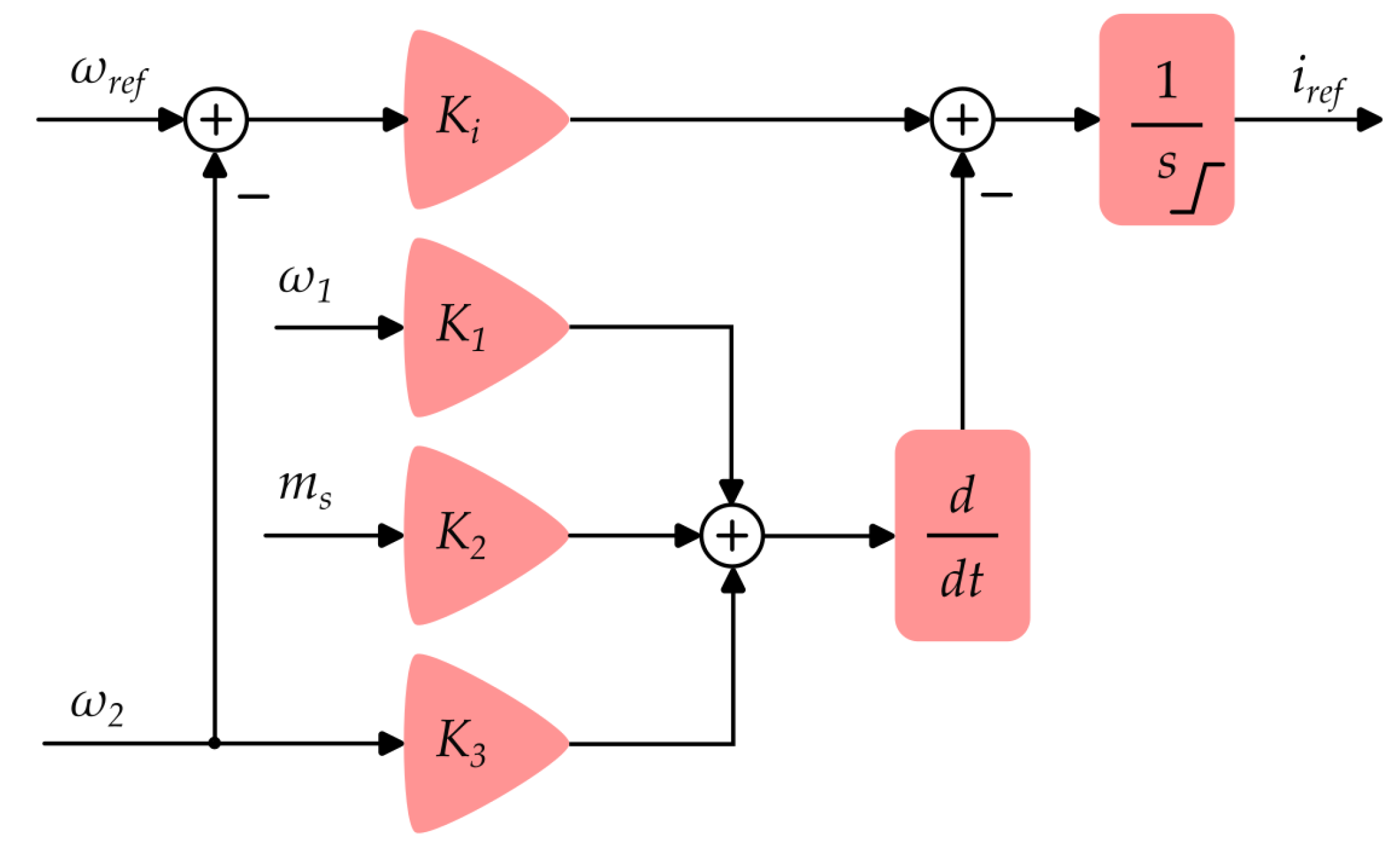
However, when calculations are performed according to Equation (5), a problem with designing a proper way of limiting the output of the controller arises. The limits for the output of the integral as well as the final output of the controller must be set either empirically or using optimization methods. A simpler solution is to move the integral past the subtraction (as shown in Figure 3), making the limit of the integral simultaneously restrain the output of the controller. Further, with this change, Equation (5) is altered and is rewritten as:

Figure 3.
A classical state feedback controller applied for two-mass system speed control.
In this manuscript, after the mathematical description of Radial Basis Function Neural Networks, applications of virtual signal generators based on neural networks in the State Feedback Controllers are presented. Two proposed structures are analyzed:
- Application of the signal from the neural generator as an additional virtual state variable;
- Replacement of one of the state variables (—shaft torque) with the neural network.
At this point in the article, an additional comment related to the function of the neural mode should be provided. The main goal is to improve the properties of the SFC controller using an adaptive element in data processing. The task of the neural network is to constantly solve the system of equations in order to search for a solution that can improve the precision of control. This should not be confused with a specific state-variable estimator.
2.2. Operating Principles of Virtual Signal Generators Based on the RBFNN
Radial Basis Function Neural Networks are a specific type of feedforward neural network. In their basic form, they always pass information from their inputs to their output. There are two distinctive features that separate this type of network from others: first, they always consist of one hidden layer; and second, the activation function of the hidden neurons is bell-shaped, meaning it monotonically decreases the further it is from the center. Usually, a Gaussian or other similar exponential function is selected. A visual representation of an RBFNN’s structure is presented in Figure 4.
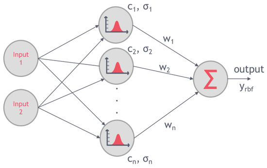
Figure 4.
Example of a Radial Basis Function Neural Network structure.
The output of each of the hidden layer neurons in the network can be calculated as [50]:
where is the input vector, is the i-th center vector, is the Euclidean norm, is the Gaussian function prescaler, and k is the iteration counter. The output of the neural network is a weighted sum of all the neurons’ outputs, given as:
The weights are updated using a gradient descent algorithm. The error function E is first defined as [51]:
where is a reference value from a model. Its value is obtained by passing the input signal through a transfer function, which can be described with the following equation:
with being the resonant frequency of the desired behavior of the reference model and being the desired damping coefficient. New values for weighted connections in the neural network are calculated as a sum of the current value of w and a correction coefficient :
The correction coefficient is defined as:
In this article, the RBFNN structure is constructed as follows: the hidden layer is comprised of five neurons, and the centers of radial basis functions are distributed equally in a range between <−1, 1>. The width of each activation function is equal to . Weights between the hidden and output layers are initiated randomly in a range between (0, 0.01). Low values of weights help mitigate the impact of a wrong starting point. Inadequate setting of weights might result in a dangerous oscillatory response during the start of the drive. The input vector is comprised of four signals: motor speed and load speed from both the current (k) and the previous () iteration.
2.3. Scenario 1—Radial Basis Function Neural Network Acting as an Additional Virtual Signal Generator
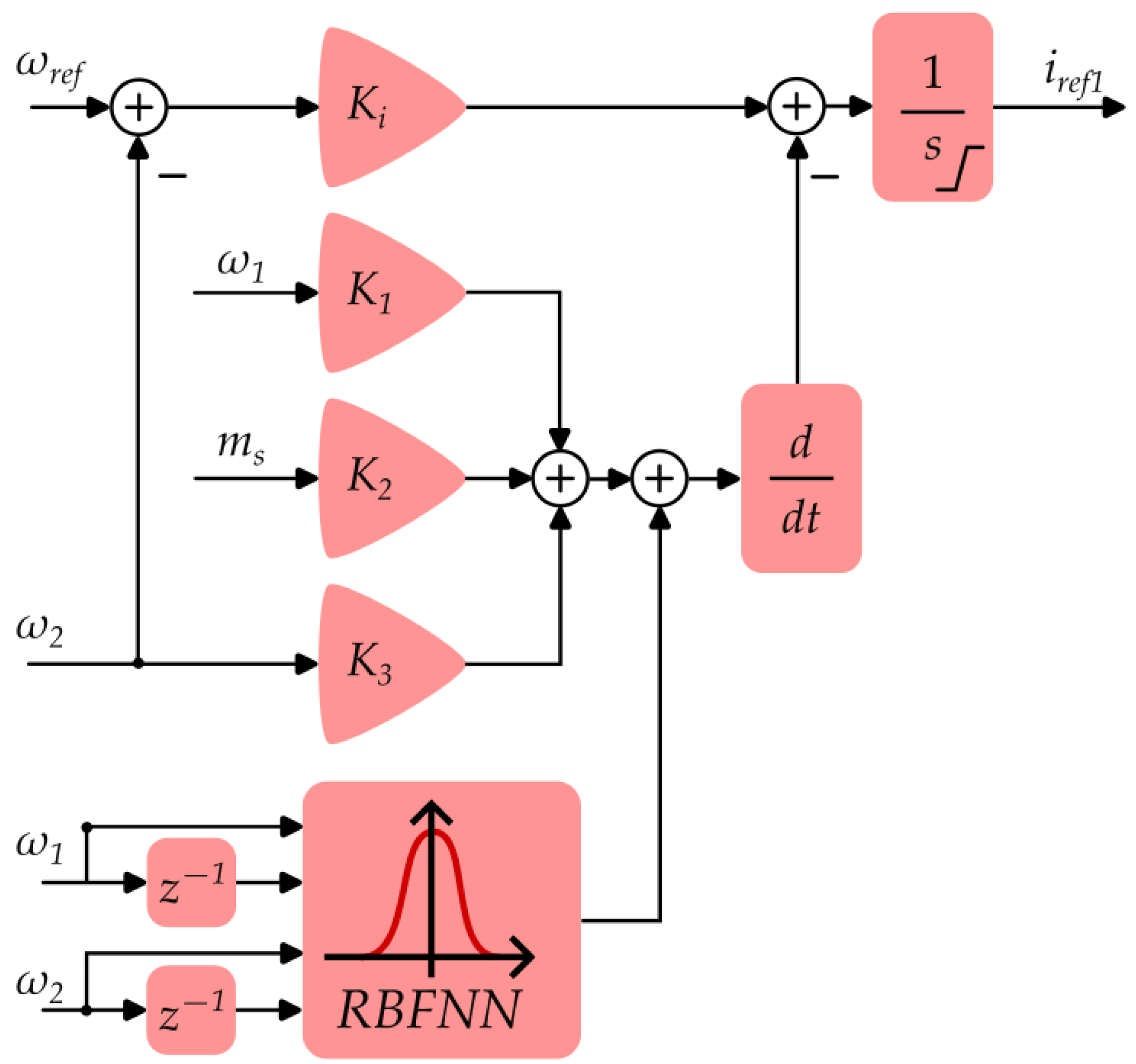
The first proposed structure introduces the RBFNN as a virtual signal generator that is complementary to all the other state variables. The addition is inspired by the Active Disturbance Rejection Control (ADRC) strategy [52]. Usually, for ADRC to be implemented, an additional extended state observer needs to be included in the control structure. In this case, the RBFNN serves as the correction mechanism to help withstand the disturbances that affect the controlled plant. The aim of the addition of the RBFNN is to generate a virtual signal that aids the control structure to mitigate the effect of parametric uncertainties (e.g., increased inertia of the load machine). The output of the controller with a parallel combination of state variables and an RBFNN output can be defined as follows:
Visual representation of this equation is shown in Figure 5. In this scenario, the RBFNN is connected in parallel with all the other state variables in the state feedback controller and acts as a compensator for any parametric uncertainties that can occur during the operation of the drive.
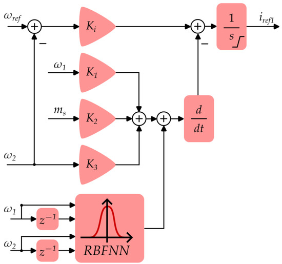
Figure 5.
The SFC with an RBFNN applied as a virtual signal generator—additional signal (related to disturbance) used in the state vector.
One of the most important stages in the design of control systems based on tunable parameters is the analysis of error behavior/changes after subsequent steps of calculations. According to such considerations, characteristic conditions are obtained that ensure the convergence of the algorithm (especially important in transient states of the control structure). For this purpose, the Lyapunov candidate function is considered as an error function and defined as:
Function V is always positive; therefore, to ensure stability and convergence of the error in the proposed control structure, the derivative , which can be also represented as a change in the error function, must always be negative:
To find the conditions for which the control structure is stable, the derivative must be solved:
with the change of error being described as:
where is the weight coefficient matrix; this can be rewritten into the following equation:
Afterwards, with the following substitution (equivalent to Equation (16)):
Equation (22) can be transformed into:
which can be further simplified into:
where:
With always being positive, the only possibility for the Lyapunov function candidate derivative to be negative is to ensure that is negative:
Therefore, to ensure stability of the system, the learning coefficient must be selected from a range between:
The lower limitation comes from the fact that needs to have a positive value. Otherwise, Equation (23) would not be fulfilled and thus stability could not be guaranteed.
2.4. Scenario 2—Radial Basis Function Neural Network Acting as a Substitute for Torsional Torque Feedback
With RBFNN used in the configuration analyzed in this subsection, numerous advantages are expected to be achieved. The inspiration for this application is taken from the fact that torsional torque is extremely difficult to measure. In typical industrial applications, there is little to no space for mounting a sensor on the flexible part of the mechanical structure. Additionally, because of rapid changes in torque behavior, obtaining a high level of precision in estimation of this signal is challenging. By substituting this signal with an RBFNN, the problem with measuring or estimating this signal is completely eliminated. The neural virtual signal generator is responsible for creating a signal suitable for the current state of the drive. It is important to highlight that in this scenario, RBFNN does not operate as a torsional torque estimator. Instead, it produces a signal that is the most suitable to achieve the desired behavior of the plant. With fewer variables and less equipment, the reliability of the control structure is increased. Furthermore, with an RBFNN, adaptive properties are expected to support the control structure when parametric uncertainties arise. For this case, the schematic for the RBFNN speed controller is shown in Figure 6. The reference signal for the torque control loop is established as:
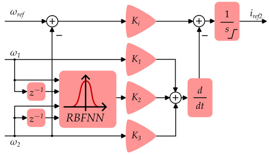
Figure 6.
The proposed state feedback controller with an RBFNN applied as virtual signal generator with elimination of the connection from the torsional torque.
Because the structures are similar, most of the derivations during the design process are identical to the ones presented for the previous case. The only difference lies in the position of the RBFNN and thus the way the derivative of the error with regard to the weight matrix changes. Thus, calculations are performed in the same manner, with the final restriction being established by Equation (29).
3. Numerical Results
The simulation tests were realized in a MATLAB/Simulink environment. Models for all the presented structures were first created. The neural network, the state feedback controller, the two-mass system, as well as the learning algorithm were all implemented using standard library blocks only. This assumption allowed us to gain full access to the parameters and signals in the control structure. The calculation step was selected as s, with Euler’s method selected as the solver.
The parameters of the drive are shown in Table 1. The drive’s mechanical time constants were identified through its step response. With this, more-accurate representation of the drive’s behavior can be expected from the simulation studies. The output of the speed controller was limited to 2.5 times the nominal current value.

Table 1.
Parameters of the analyzed two-mass system.
The following subsections focus on the analysis of the obtained results for the two tested control schemes (combinations of adaptive RBFNN and the SFC). The difference between them is the place where the output of the network is combined with the classical controller. According to the assumption that RBFNNs are tools adequate for tasks of interpolation and approximation (and therefore finding a relation between the input and the output signals), adaptive properties should be observed when parametric uncertainties are introduced. Further, the response to external disturbances is tested during numerical studies. At s, the nominal value of load torque is triggered, and later, at s, the load torque is deactivated.
The aim of the virtual signal generator is to produce a sub-control signal that is adequate for the current state of the drive. When parametric uncertainties arise, the RBFNN should produce a signal that counteracts the effect of improperly selected gains () of the state feedback controller. It is worth noting that even though the virtual signal acts as an additional state variable, it does not have any physical interpretation. Therefore, no unit can be assigned to it.
3.1. Scenario 1—Radial Basis Function Neural Network Acting as an Additional Virtual Signal Generator
The first proposed structure uses the RBFNN as an additional virtual state variable generator. The output of the network is combined with the other state variables before all of them are fed through the derivative operator. The visual representation of the proposed adaptive controller is shown in Figure 5.
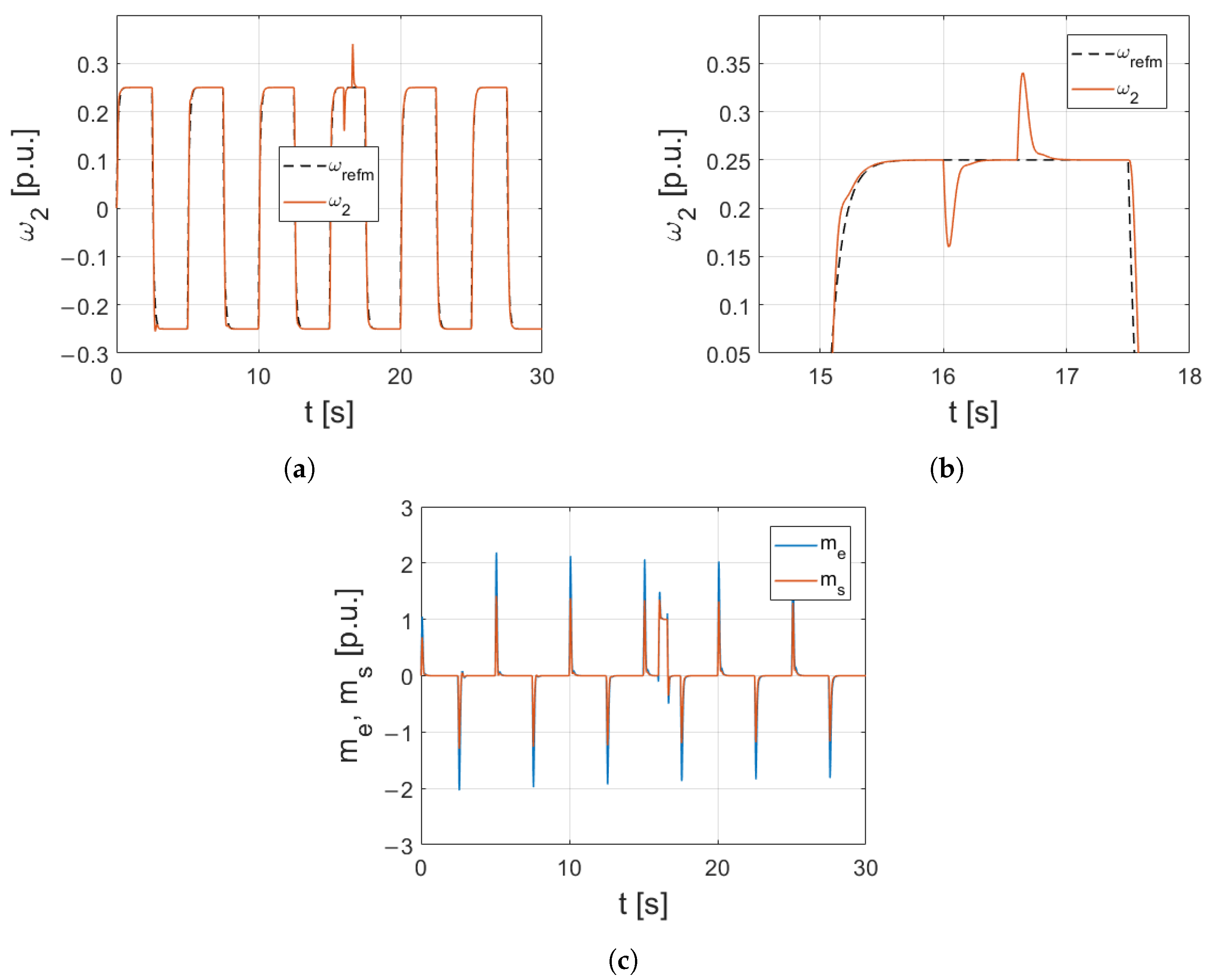
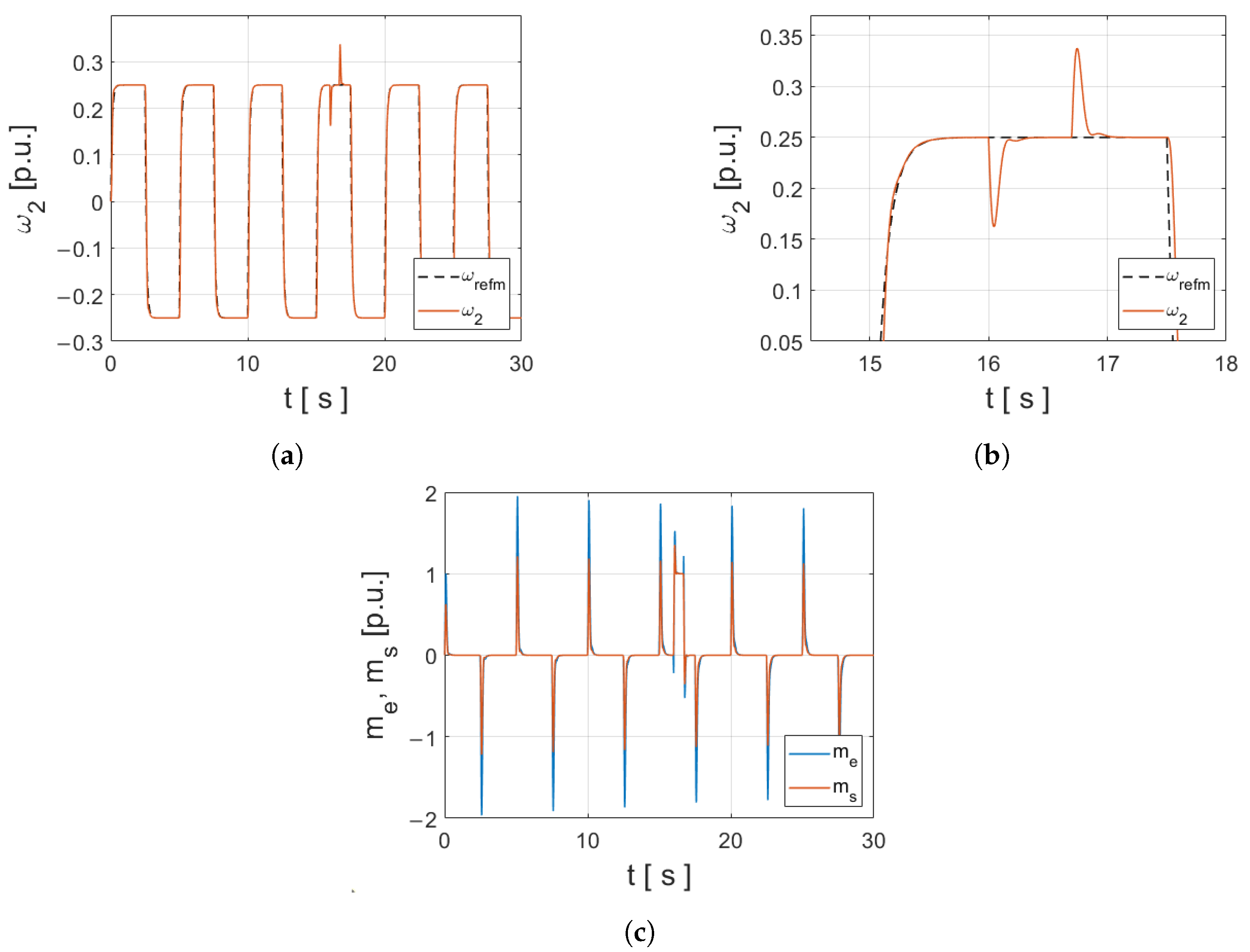
First, a general overview of the proposed structure’s operation is presented. The drive’s parameters are set to their nominal values (no parameter uncertainty is introduced). Load speed as well as electromagnetic and torsional torque transients are shown in Figure 7. The load machine follows the reference speed from the model with great precision. The response is dynamic and is not delayed. The drive’s response to external load torque (shown in Figure 7b) is also quick and does not introduce much of an overshoot. Electromagnetic torque spikes do not last long and are kept within the limit. Thanks to that, no overshoot is present. The slight mismatches between the reference and actual speed that can be observed in the initial stage of the drive’s operation are a result of randomly selected weight coefficients. That mismatch is gradually reduced thanks to the learning algorithm, which indicates that the adaptive properties are present in the analyzed structure. To facilitate smoother starts for the drive, the initial parameters of the neural network should be optimized, e.g., with nature-inspired algorithms [53].
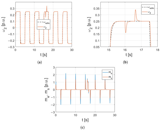
Figure 7.
Simulation results for Structure 1: (a) Load machine speed transient. (b) Close-up showing the system’s reaction to load torque. (c) Electromagnetic and torsional torque.
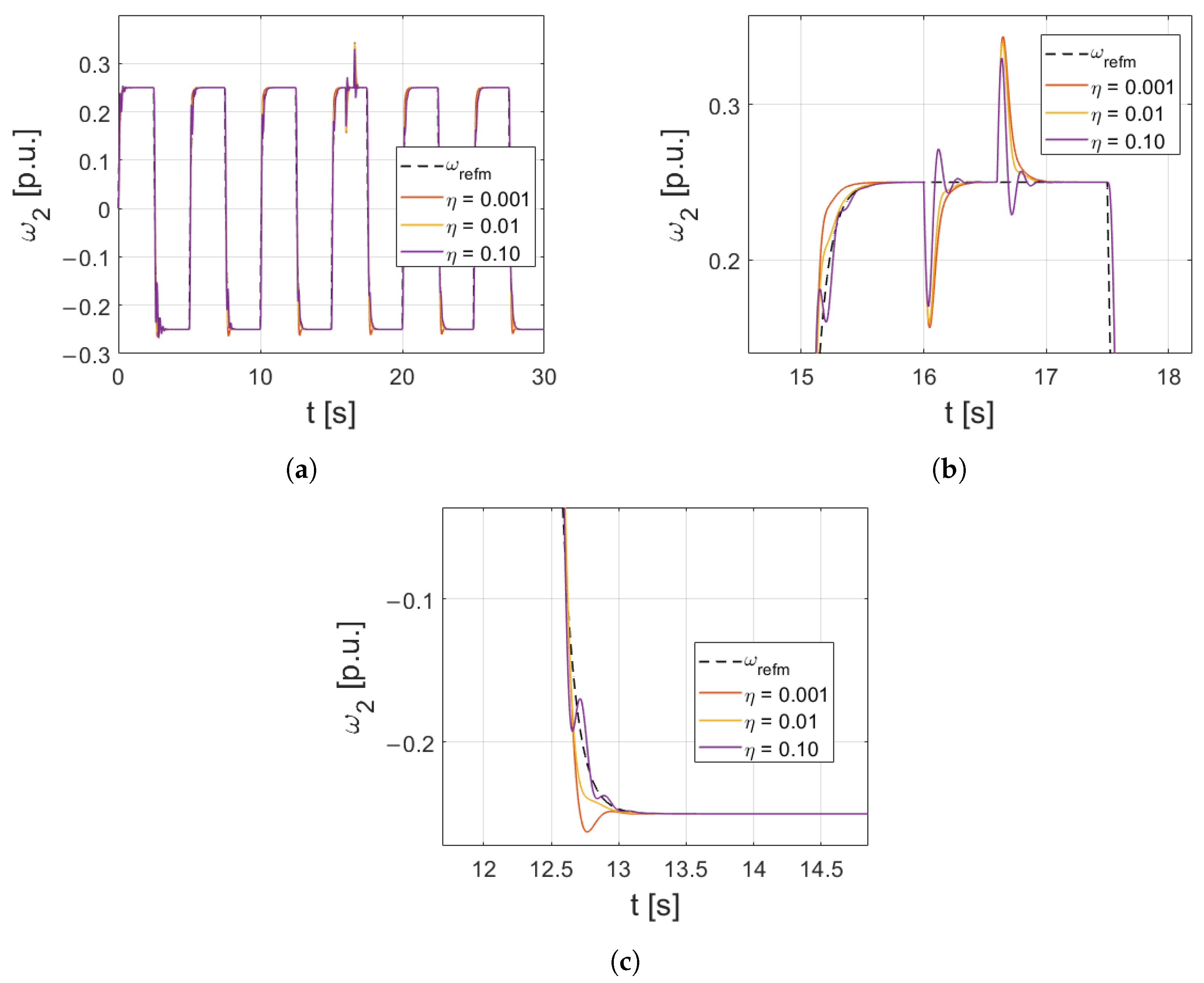
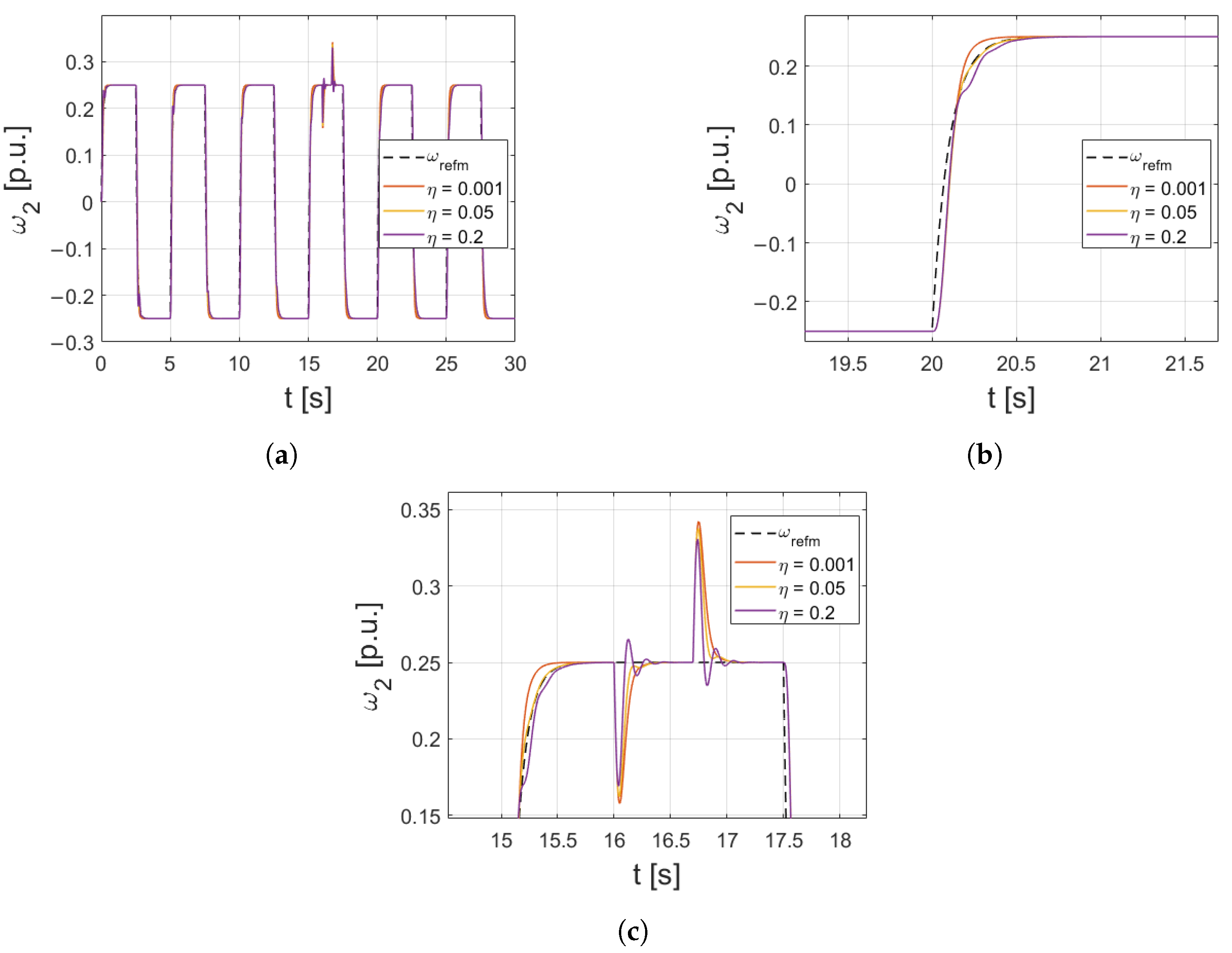
Further analysis of the control structure investigates the influence of the learning coefficient . Load speed transients are presented in Figure 8. A lower value of this parameter translates into quicker settling and smaller overshoot when the machine is turning one way (Figure 8b) but slower settling when turning the other way (Figure 8c). It is also characterized by the biggest overshoot when load torque is introduced. On the other hand, when is selected with a bigger value, load speed very precisely follows the reference value in one direction but has the most oscillatory response when turning the opposite direction. The middle value provides the best response to the load torque—it is not oscillatory (as for the bigger value) and the settling time is quicker than for the smaller one. It can be stated that for this structure, the learning rate should be either carefully selected (with regard to the application, the possible presence of intense load torques, etc.) or optimized.

Figure 8.
Comparison of the impact of different values of the learning coefficient on the performance of the drive with Structure 1: (a) Full simulation run. (b) Close-up showing the system’s response to the load torque. (c) Close-up showing one of the reversions.
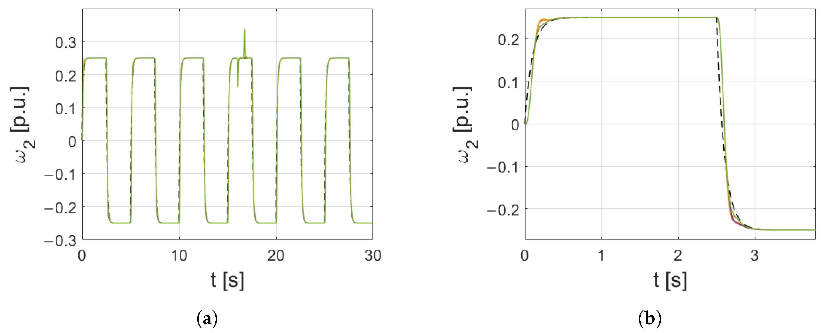
Figure 9 illustrates the effect of the initial values of the weights on the operation of the drive. The weights were randomly selected from the range between 0 and 5 to enable the possibility of starting the drive from a disadvantageous state. Random selection of weights does not heavily influence the drive’s operation. Neither oscillations nor any big overshoots can be seen. After some time, with training, the transients begin to look alike due to the weights being changed to reach a better control signal. For the initial weights, optimization or preliminary training is suggested but is not mandatory.
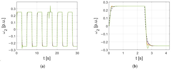
Figure 9.
Impact of different starting points for RBFNN’s weight coefficients on the performance of the drive with Structure 1: (a) Full simulation run. (b) Close-up showing the initial stage of the drive’s operation.
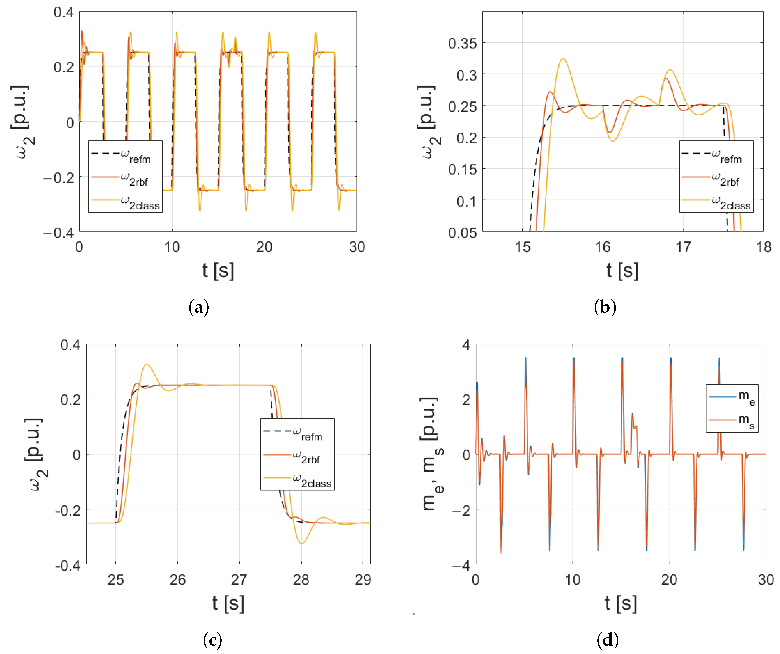
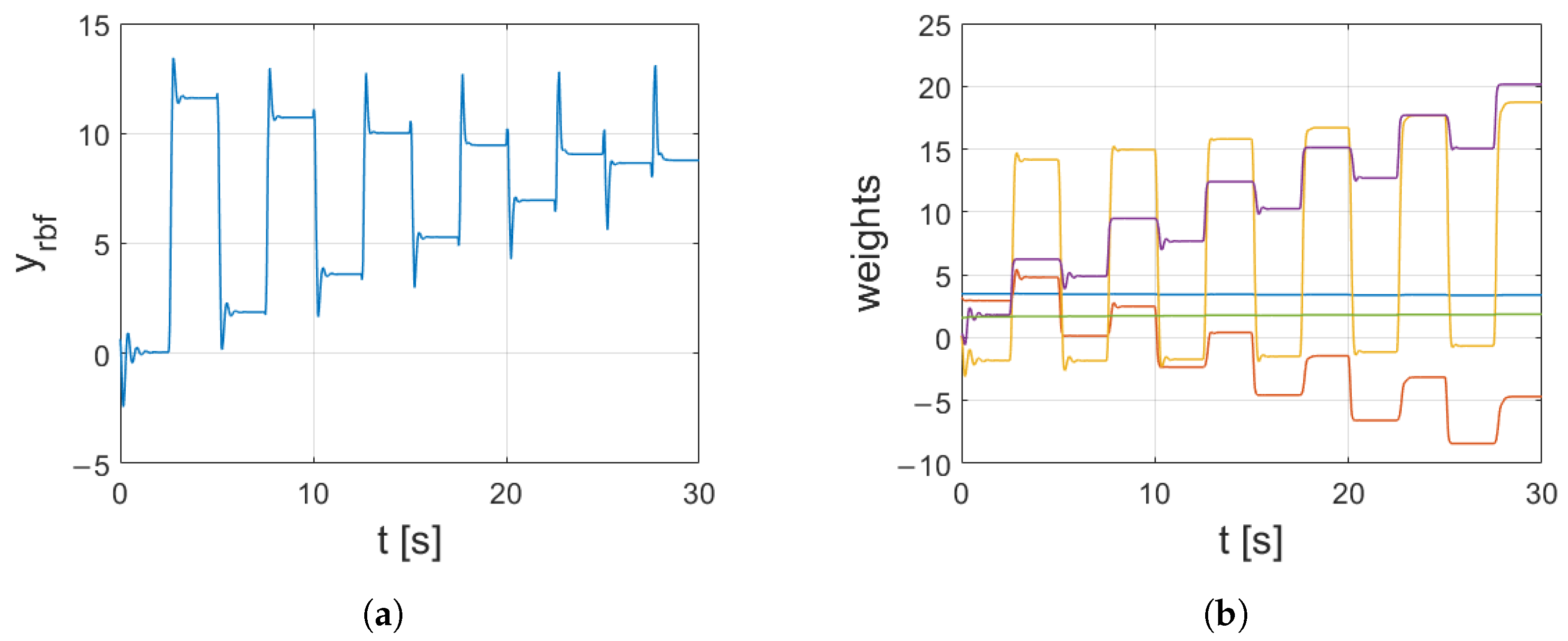
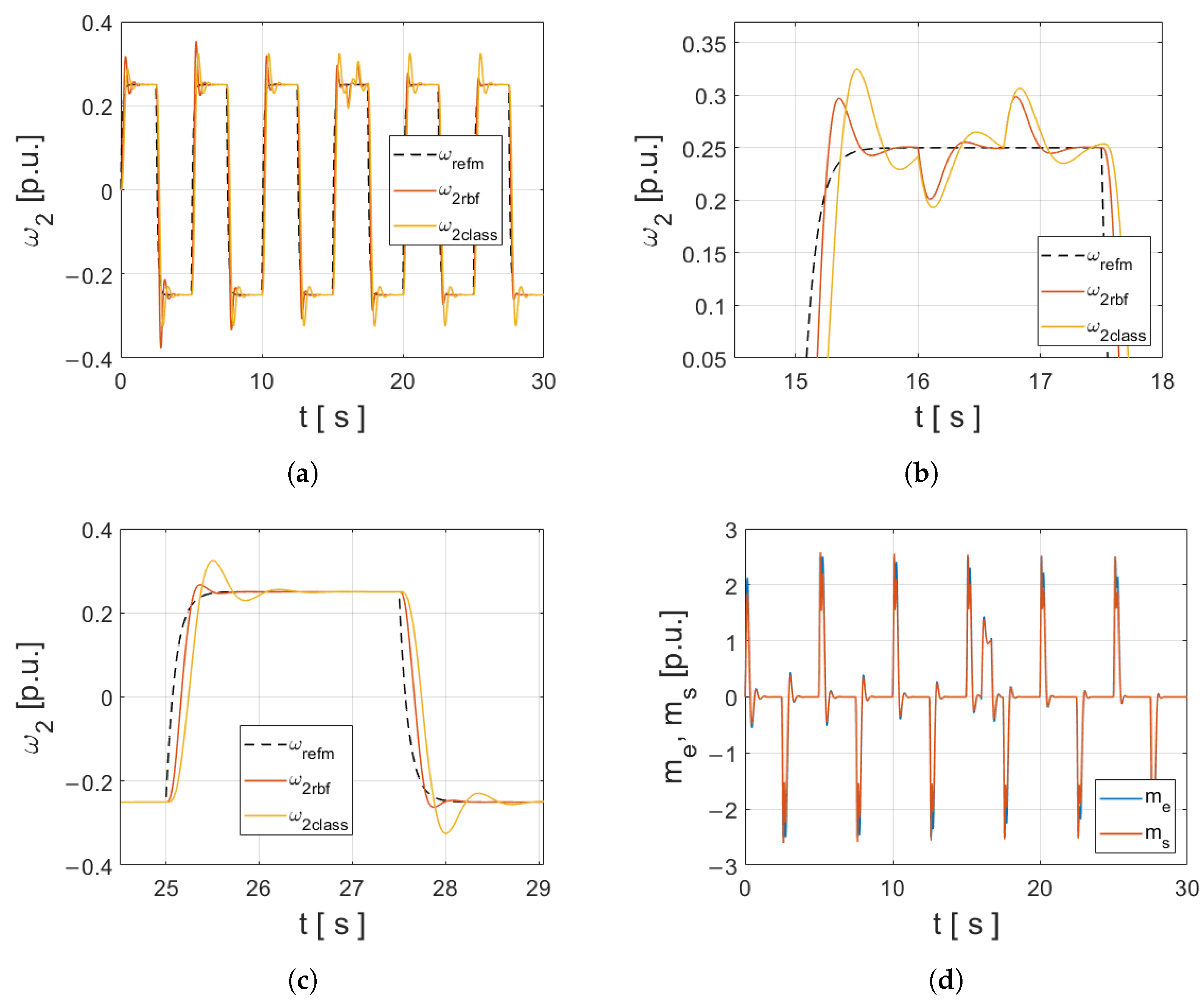
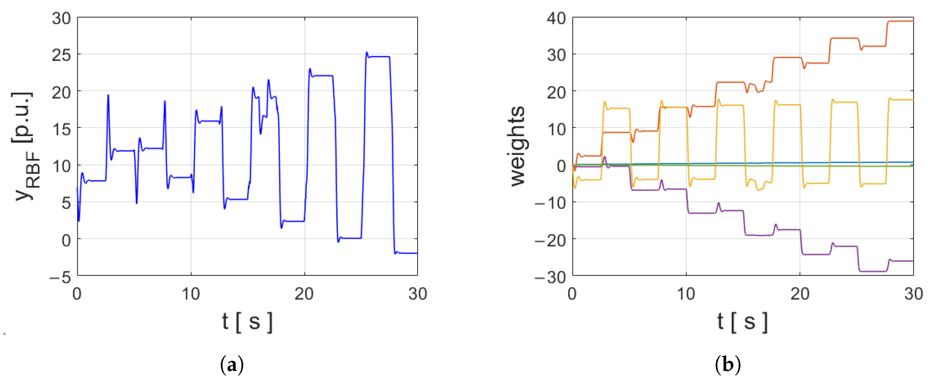
Finally, operation under parameter uncertainty is examined. The change is modeled by increasing the time constant (inertia) of the load machine four times. Figure 10 shows transients of the drive’s state variables (compared to the results obtained for a classical State Feedback Controller), while Figure 11 shows transients of the RBFNN virtual state variable generator signals: its output and weights. The results are also compared with the response of a classical State Feedback Controller to show the scale of the achieved improvement. Overshoots and oscillations, which result from the gain of the controller being set inadequately for the inertia of the load machine, are progressively suppressed. Changes in the network’s weights and outputs can also be observed. It can be stated that the addition of the neural virtual signal generator aids the process of two-mass drive control in the presence of parametric uncertainty.

Figure 10.
Simulation results for Structure 1 operating under parameter uncertainty ( increased four times): (a) Load machine speed transient. (b) Close-up showing the system’s reaction to load torque. (c) Close-up showing system’s response during last reversions. (d) Electromagnetic and torsional torque.
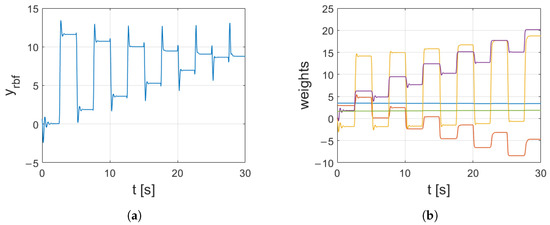
Figure 11.
Radial Basis Function Neural Network parameters during the operation of the drive under parameter uncertainty ( increased four times): (a) Output of the RBFNN. (b) Transients of weight coefficients.
3.2. Scenario 2—Radial Basis Function Neural Network Acting as a Substitute for Torsional Torque Feedback
In this scenario, the RBFNN serves as a substitute for the torsional torque. It is a promising solution mainly because torsional torque is difficult to measure. If substituting it with a virtual variable from a neural network proves to be a good alternative, the reliability of the drive can be improved. The drive’s operation is no longer dependent on the accuracy of the estimation of the torsional torque. Moreover, if the drive is equipped with torsional torque measurement devices, they can all be eliminated, lowering the cost of the drive and the necessity to perform maintenance (also, without these devices, there are fewer elements that can fail or be damaged).
Firstly, the system’s operation under nominal parameters of the drive is verified. The obtained transients of the load angular speed and electromagnetic and torsional torque are presented in Figure 12. The reference speed is followed with high precision. Moreover, no oscillations can be observed. Slight misalignment is present in the beginning stages of operation due to the weights still not being adapted to adequate values. The system’s response to load torque is non-oscillatory and rapidly returns to following the reference value without any overshoot.
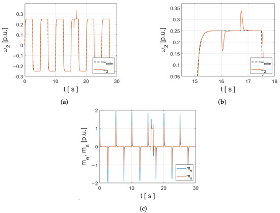
Figure 12.
Simulation results achieved for the adaptive control structure without the connection from torsional torque: (a) Load machine speed transient. (b) Close-up showing the system’s reaction to load torque. (c) Electromagnetic and torsional torque.
The following test is focused on examining the impact of the learning rate on the drive’s performance. The results shown in Figure 13 prove that the value of this parameter plays a crucial role. Bigger values cause observable oscillations, which are most prominent during the switching of the load torque. With lower values, the impact is not that significant; however, a slight delay can be observed due to the slower adaptation of the control structure. As in the previously inspected structure, it is also highly advised to optimize this parameter to the target plant in this case.
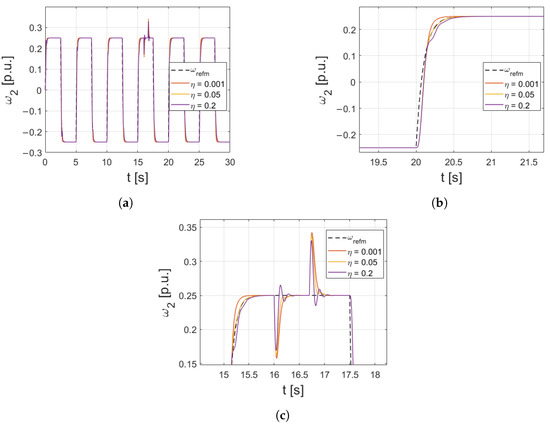
Figure 13.
Impact of different values of the learning coefficient on the performance of the drive: (a) Complete simulation run. (b) Close-up showing the initial stage of the operation of the drive. (c) Zoom showing the system’s response to the load torque.
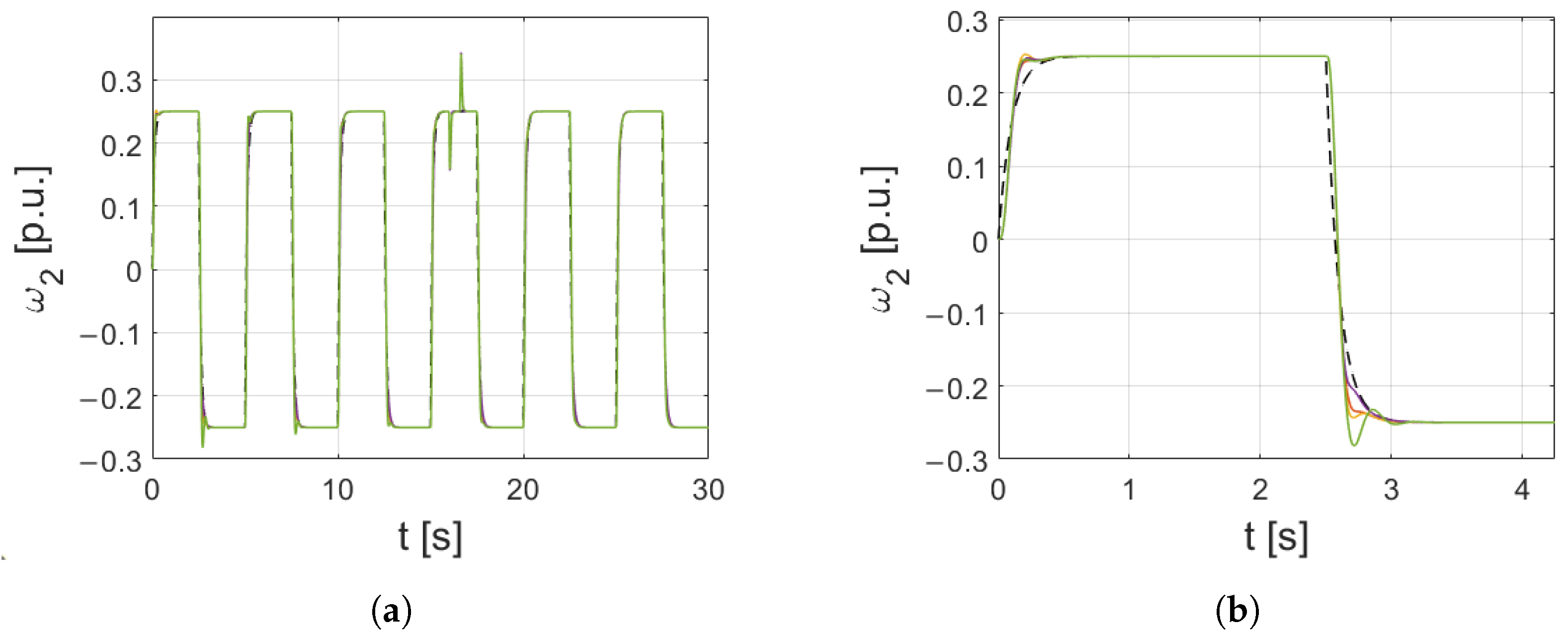
The next test was carried out to examine the impact of the initial weights of the neural network, the results of which can be observed in Figure 14. The initial weights were selected at random from a range between 0 and 10 (instead of between 0 and 0.01). The transients show that the initial weights do not significantly change the performance of the drive. Still, the initial parameters of the RBFNN can be optimized to eliminate the oscillations in the early stages of operation.
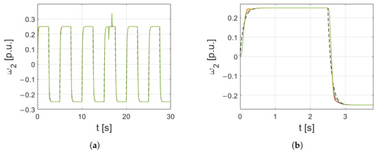
Figure 14.
Comparison of the impact of different values of the initial weights on the performance of the drive with the analyzed control structure: (a) Complete simulation run. (b) Close-up showing the initial stage of the operation of the drive.
Finally, the impact of parameter uncertainty was tested. As in the previous case, the parameter uncertainty was introduced as a quadruple increase in the load machine’s inertia. The obtained results can be seen in Figure 15. The related response of the RBFNN is shown in Figure 16. Results show great adaptation to the new working environment. The impact of the increase in inertia is almost completely mitigated by the RBFNN output. The initial oscillations are completely dampened. The operation during dynamic states is also satisfactory.
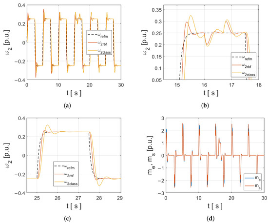
Figure 15.
Simulation results for the tested control structure: (a) Load machine speed transient. (b) Close-up showing the system’s response to load torque. (c) Close-up showing the system’s final reversions. (d) Electromagnetic and torsional torques.
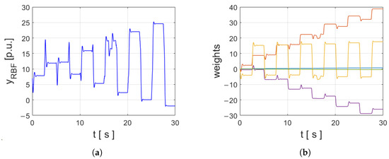
Figure 16.
Radial Basis Function Neural Network parameters during the operation of the drive under parameter uncertainty ( increased four times): (a) Output of the RBFNN. (b) Transients of weight coefficients.
4. Experimental Results
Consequently, experimental verification of the presented numerical results is carried out. The experimental bench used for this purpose is comprised of two DC machines interconnected with a 595 mm-long steel shaft, which is 6 mm in diameter. In this way, an elastic connection between the motors is established. Moreover, the inertia of the load machine can be adjusted by mounting additional weight plates on the load machine side of the shaft. The armature current is measured with an LEM current transducer. Speed of both machines is measured with 36,000 pulses-per-revolution incremental encoders. The motor is powered through an H-bridge driver. The tested control algorithms are implemented in a dSpace 1103 fast prototyping card using a MATLAB/Simulink environment. The whole laboratory setup is shown in Figure 17.
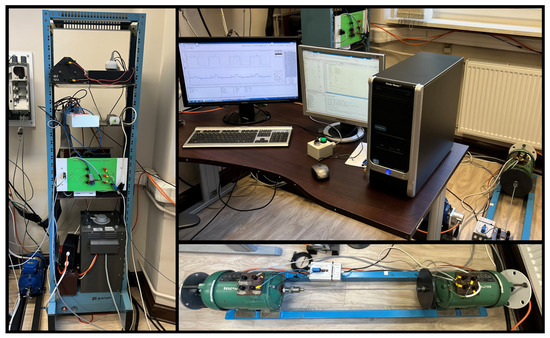
Figure 17.
The laboratory equipment.
4.1. Scenario 1—Radial Basis Function Neural Network Acting as an Additional Virtual Signal Generator
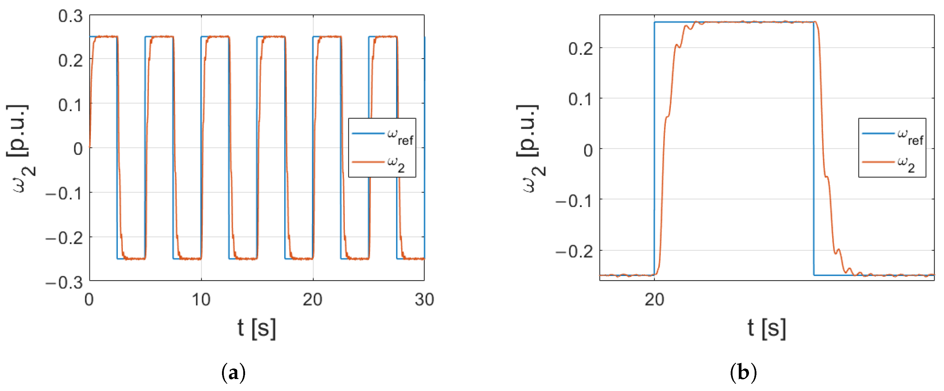
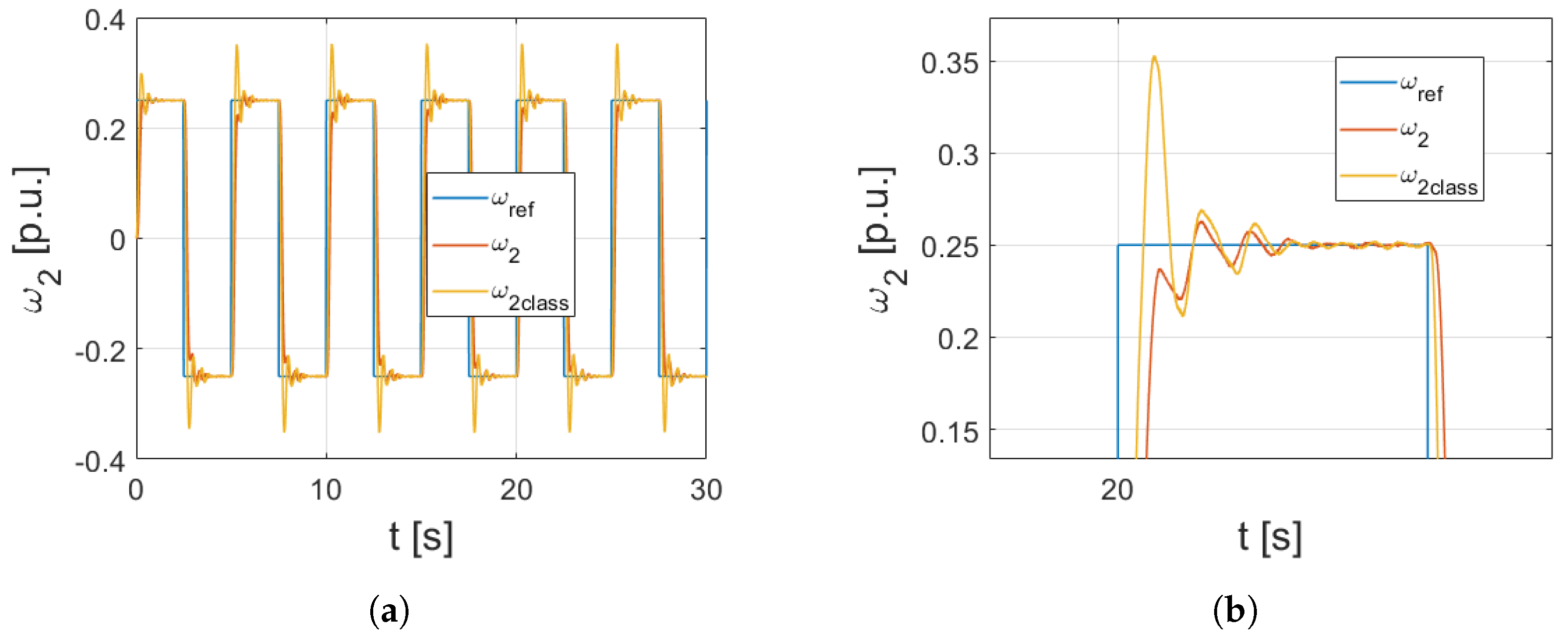
The first experimental verification was conducted for the structure with the fourth neural virtual signal. Figure 18 presents the operation of the drive with nominal parameters. Transients for this structure transpired to be quite oscillatory. Still, the response was stable and the oscillations were slowly being dampened during the operation of the drive. What showed promise, however, was the response to a structure with parametric uncertainty (increased inertia of the load machine). The results are demonstrated in Figure 19. The overshoots caused by the improper selection of the parameters of the state feedback controller were gradually minimized by the RBFNN. What can be observed is that after just 25 s of operation, the overshoot was reduced by almost 50% (Figure 19b). Moreover, with the lower overshoot, the settling time was also shortened.

Figure 18.
Experimental verification of the operation of Structure 1: (a) Full experimental transient. (b) Close-up showing a single reversion.
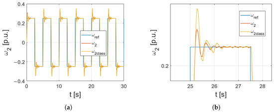
Figure 19.
Experimental verification of the operation of Structure 1 under parameter uncertainty compared to a classical state feedback controller: (a) Full experimental transient. (b) Close-up showing a single reversion.
4.2. Scenario 2—Radial Basis Function Neural Network Acting as a Substitute for Torsional Torque Feedback
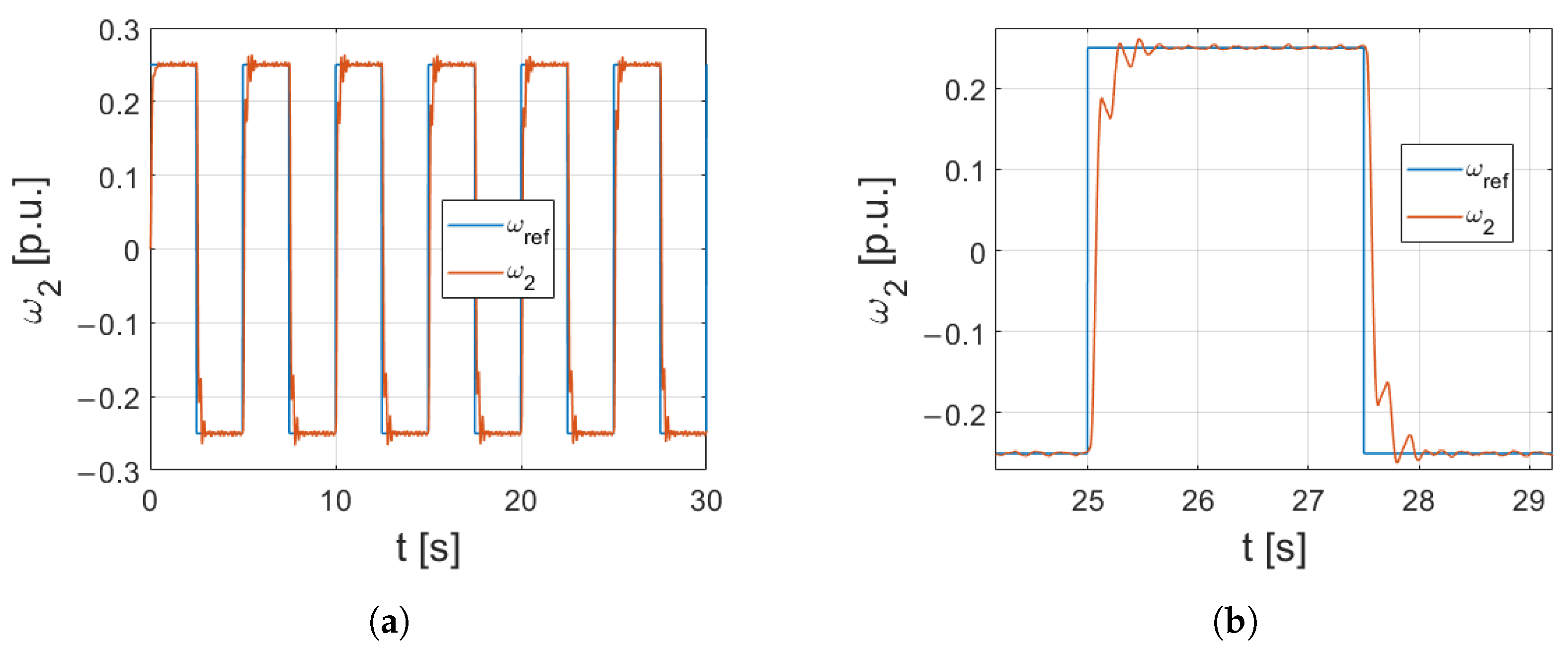
The experimental tests for the structure with the RBFNN substitute for torsional torque were next performed. The obtained transients are shown in Figure 20. The response was subtly oscillatory; however, it does not produce any overshoot and smoothly transitions to the reference value.
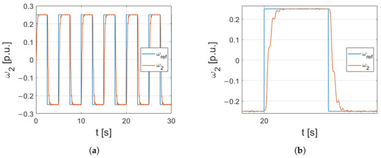
Figure 20.
Experimental verification of the operation of Structure 2: (a) Full experimental transient. (b) Close-up showing a single reversion.
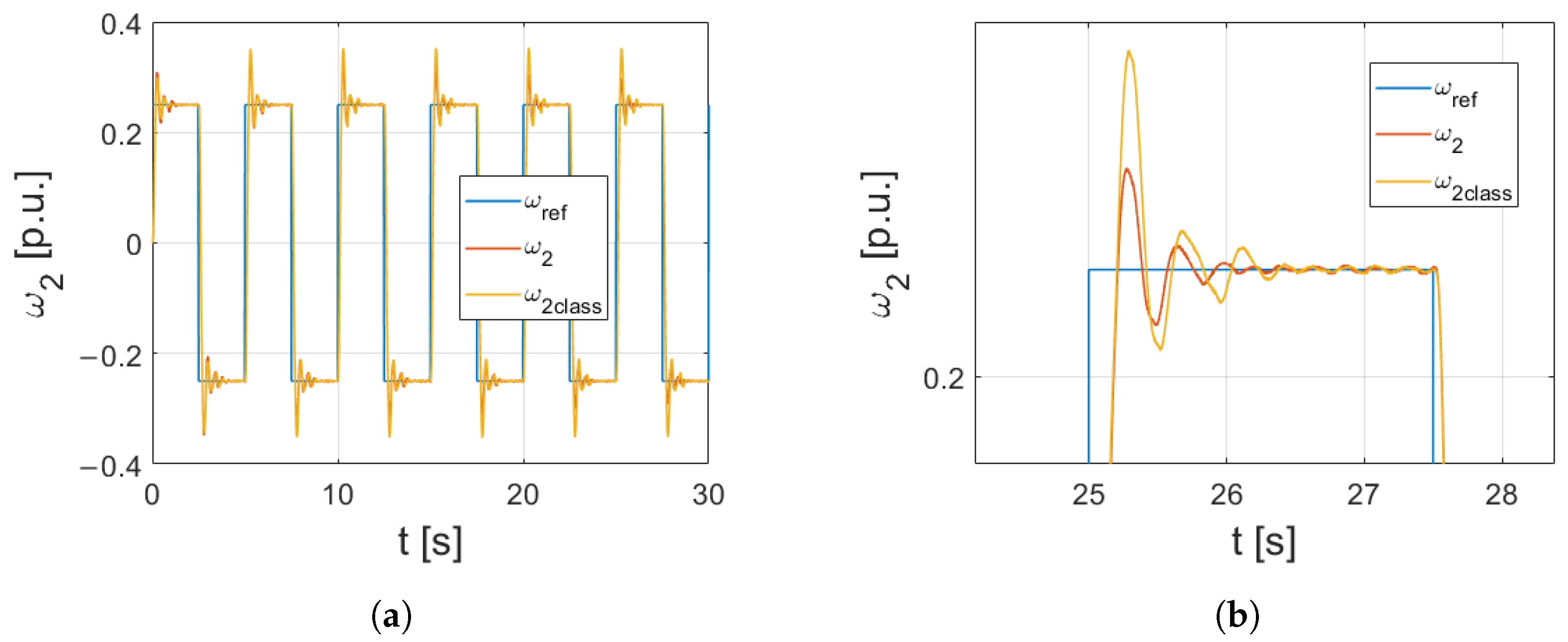
The biggest contribution of this structure is its response to parametric uncertainty. Figure 21 presents the experimental transients for this case. The first finding is that the structure almost instantly recognizes the increased inertia of the load machine. There is no overshoot from the very beginning of operation. The response is lightly oscillatory, but it still is a great improvement from the classical state feedback controller, which can be seen in the figure.
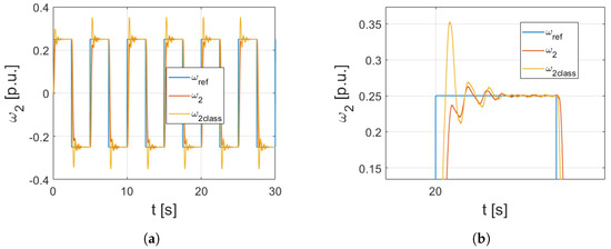
Figure 21.
Experimental verification of the operation of Structure 2 under parameter uncertainty compared to a classical state feedback controller: (a) Full experimental transient. (b) Close-up showing a single reversion.
4.3. Comparison of the Obtained Results
In order to provide a fair basis for comparison of the presented transients, an integral criterion has been calculated for each of the tested cases. The criterion selected for this study is the Integral Absolute Error (IAE) calculated as follows:
where is the duration of numerical and experimental tests ( s), and
Trapezoidal numerical integration was performed to obtain the approximate values of . Table 2 presents the results of the comparison.

Table 2.
Integral Absolute Error (IAE) values for simulation and experimental tests.
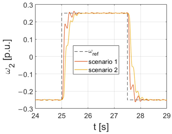
According to the IAE criterion, the control algorithm from Scenario 1 (RBFNN virtual generator providing an additional signal) outperforms the other control structure, especially in the experimental tests. The visual comparison of the obtained results is shown in Figure 22. The results obtained with the control structure shown in scenario 1 are characterized by a more-aggressive response. The angular speed of the load machine changes more quickly, and therefore, the calculated error is smaller. The control structure from Scenario 2 has a more temperate response but is not as oscillatory. In addition to the general conclusions regarding the analyzed control structures, it should be noted that the classic structure with a state controller was omitted in the comparison. This is due to the fact that the efficiency of the classical state controller with constant parameters (especially after changes in the object parameters) was significantly improved (in each case) by introducing the RBFNN (Figure 19 and Figure 21).
5. Conclusions
This article proposes two alternatives for possible use of Radial Basis Neural Networks in speed control of two-mass systems. In each of these cases, the RBFNN was used to mitigate the presence of parametric uncertainty (i.e., increased inertia of the load machine). Adaptive properties were visible and positively influenced the operation of the drive in all of the presented structures. The adaptive RBFNN state feedback control structures introduce the advantages/features described in the remarks below:
- The main contribution of this paper is the development of new control algorithms, which significantly improve operation of classic State Feedback Controllers applied to two-mass systems in the presence of parameter uncertainty. The best experimental results, considering full elimination of overshoot, were achieved for the structure with the RBFNN acting as a substitute signal for torsional torque.
- Thorough examination revealed that the presented control structures are stable and the change in weights provided by the adaptation algorithm ensures that the control error converges to zero.
- All the analyzed structures were comprehensively verified. Both numerical and experimental tests (electric drive simulating operation of real industrial applications) prove a positive impact of the analyzed control algorithms (proposed modifications).
- None of the presented cases is negatively affected by the random selection of the starting point. Still, to facilitate smooth operation in the early stages of operation, pre-optimization is recommended.
- According to the stability analysis as well as the numerical examination of the proposed control algorithms, selection of the learning coefficient is highly important. Even small changes in this parameter can produce apparent changes in the operation of the drive. It is advised to perform additional optimization of the learning rate to obtain the best result for a given application.
- Another advantage of the presented modifications used in the algorithms (based on reconfigurability) is the model-free approach. Without any state observer, no additional recalculation of the plant parameters needs to be performed to adapt to the current state of the drive.
- The structure with RBFNN acting as a substitute for the torsional torque provides one additional asset. When information about torsional torque is excluded from the control structure, there is no need for measurement (which is difficult if not impossible to implement) of this signal. Strain gauges configured in a Wheatstone bridge are most often used for torque measurement. This solution suffers from multiple drawbacks. The bridge needs to be connected to the chassis of the sensor through brushes, which are an additional source of friction (and therefore heat). Strain gauges are highly sensitive to temperature changes, making torque measurements with this method less precise. Optical torque sensors are also available; however, they are significantly more expensive and harder to maintain. Elimination of torque sensors reduces the cost of the drive and makes it more reliable. Further, substituting estimation of the torsional torque with the RBFNN additionally provides adaptive properties, making the control structure more versatile and prone to parameter changes without drastically increasing the computational complexity of the algorithm.
6. Discussion
Continuation of this research will be directed towards optimization of the parameters of the RBFNN. Meta-heuristic, nature-inspired algorithms will be considered to find an advantageous initial point for the weight coefficients and the learning rate, while gradient-based or other clustering methods can be investigated to search for the proper design of activation function parameters (distribution of the centers and selection of widths for individual neurons). Observation of the behavior of the weights in each structure shows that there is always a pair that almost do not change their values (in a mirroring fashion). This behavior may suggest that their respective neurons are not highly activated (low value of due to a considerable distance between the input and center vectors). The possibility of these weights being accurately adjusted cannot be fully excluded. Optimization of the neuron centers could, however, enhance the learning process for all the neurons and, as a result, provide even better speed transients.
Author Contributions
Conceptualization, M.K.; methodology, M.K. and R.S.; software, R.S.; validation, M.K., R.S. and J.-R.T.; formal analysis, M.K., R.S. and J.-R.T.; investigation, M.K., R.S. and J.-R.T.; data curation, R.S.; writing—original draft preparation, M.K., R.S. and J.-R.T.; writing—review and editing, M.K., R.S. and J.-R.T.; visualization, R.S.; supervision, M.K. and J.-R.T.; project administration, M.K. All authors have read and agreed to the published version of the manuscript.
Funding
This research received no external funding.
Data Availability Statement
Not applicable.
Conflicts of Interest
The authors declare no conflict of interest.
Abbreviations
The following abbreviations are used in this manuscript:
| ADRC | Active Disturbance Rejective Control |
| IAE | Integral Absolute Error |
| MPC | Model Predictive Control |
| MRAS | Model Reference Adaptive System |
| RBFNN | Radial Basis Function Neural Network |
| SFC | State Feedback Controller |
References
- Brando, G.; Piegari, L.; Spina, I. Simplified Optimum Control Method for Monoinverter Dual Parallel PMSM Drive. IEEE Trans. Ind. Electron. 2018, 65, 3763–3771. [Google Scholar] [CrossRef]
- Pan, X.; Wang, Y.; Qi, Y. Artificial Neural Network Model and Its Application in Signal Processing. Asian J. Adv. Res. Rep. 2023, 17, 1–8. [Google Scholar] [CrossRef]
- Ellis, G.; Lorenz, R.D. Resonant load control methods for industrial servo drives. IEEE Ind. Appl. Conf. 2000, 3, 1438–1445. [Google Scholar]
- Park, T.S.; Shin, E.C.; Oh, W.H.; Yoo, J.Y. Robust speed control for torsional vibration suppression of rolling mill drive system. In Proceedings of the 29th Annual Conference of the IEEE Industrial Electronics Society IECON’03, Roanoke, VA, USA, 2–6 November 2003; pp. 66–71. [Google Scholar]
- Rajendran, S.; Diaz, M.; Chavez, H.; Cruchaga, M.; Castillo, E. Terminal Synergetic Control for Variable Speed Wind Turbine Using a Two Mass Model. In Proceedings of the IEEE CHILEAN Conference on Electrical, Electronics Engineering, Information and Communication Technologies (CHILECON), Valapraiso, Chile, 6–9 December 2021; pp. 1–6. [Google Scholar]
- Shao, M.; Huang, Y.; Silberschmidt, V.V. Intelligent Manipulator with Flexible Link and Joint: Modeling and Vibration Control. Shock Vib. 2020, 2020, 4671358. [Google Scholar] [CrossRef]
- Zhang, P.; Li, Y. New Indices for Evaluating Vibration Characteristics of Flexible-Joint Robots. Appl. Sci. 2020, 10, 4895. [Google Scholar] [CrossRef]
- Elghoul, A.; Tellili, A.; Abdelkrim, M.N. Reconfigurable control of flexible joint robot with actuator fault and uncertainty. J. Electr. Eng. 2019, 70, 130–137. [Google Scholar] [CrossRef]
- Alam, W.; Mehmood, A.; Ali, K.; Javaid, U.; Alharbi, S.A.; Iqbal, J. Nonlinear Control of a Flexible Joint Robotic Manipulator with Experimental Validation. Stroj. Vestn. 2018, 64, 47–55. [Google Scholar]
- Zhang, X.; Qiu, J.; Zhu, J.; Li, S. A composite position control of flexible lower limb exoskeleton based on second-order sliding mode. Nonlinear Dyn. 2022, 111, 1657–1666. [Google Scholar] [CrossRef]
- Kong, D.; Wang, W.; Shi, Y.; Kong, L. Flexible Control Strategy for Upper-Limb Rehabilitation Exoskeleton Based on Virtual Spring Damper Hypothesis. Actuators 2022, 11, 138. [Google Scholar] [CrossRef]
- Koch, A.; Schulz, L.; Jakstas, G.; Falkenstein, J. Drivability Optimization by Reducing Oscillation of Electric Vehicle Drivetrains. World Electr. Veh. J. 2020, 11, 68. [Google Scholar] [CrossRef]
- Yang, G.; Liu, Y.; Jin, M.; Liu, H. A Robust and Adaptive Control Method for Flexible-Joint Manipulator Capturing a Tumbling Satellite. IEEE Access 2019, 7, 159971–159985. [Google Scholar] [CrossRef]
- Carabis, D.S.; Wen, J.T. Trajectory Generation for Flexible-Joint Space Manipulators. Front. Robot. AI 2022, 9, 687595. [Google Scholar] [CrossRef] [PubMed]
- Palleschi, A.; Mengacci, R.; Angelini, F.; Caporale, D.; Pallottino, L.; De Luca, A.; Garabini, M. Time-Optimal Trajectory Planning for Flexible Joint Robots. IEEE Robot. Autom. Lett. 2020, 5, 938–945. [Google Scholar] [CrossRef]
- Fu, X.; Ai, H.; Chen, L. Repetitive Learning Sliding Mode Stabilization Control for a Flexible-Base, Flexible-Link and Flexible-Joint Space Robot Capturing a Satellite. Appl. Sci. 2021, 11, 8077. [Google Scholar] [CrossRef]
- Choi, S.B.; Hong, S.R.; Sung, K.G.; Sohn, J.W. Optimal control of strucutural vibrations using a mixed-mode magnetorheological fluid mount. Int. J. Mech. Sci. 2008, 50, 559–568. [Google Scholar] [CrossRef]
- Brock, S.; Gniadek, M. Robust input shaping for two-mass system with variable parameters. Pozn. Univ. Technol. Acad. J. 2014, 77, 209–215. [Google Scholar]
- Ilchmann, A.; Schuster, H. PI-Funnel Control for Two Mass Systems. IEEE Trans. Autom. Control 2009, 54, 918–923. [Google Scholar] [CrossRef]
- Pai, N.S.; Kuo, Y.P. Speed control for a two-mass drive system using integrated fuzzy estimator and hybrid fuzzy PD/PI controller. J. Phys. 2008, 96, 012094. [Google Scholar] [CrossRef]
- Wrobel, K.; Nalepa, R.; Najdek, K.; Szabat, K. Design of the control structure for two-mass system with help of the D-decomposition technique. In Proceedings of the 2021 IEEE 19th International Power Electronics and Motion Control Conference (PEMC), Gliwice, Poland, 25–29 April 2021; pp. 711–716. [Google Scholar] [CrossRef]
- Zouari, L.; Abid, H.; Abid, M. Sliding mode and PI controllers for uncertain flexible joint manipulator. Int. J. Autom. Comput. 2015, 12, 117–124. [Google Scholar] [CrossRef]
- Szabat, K.; Orlowska-Kowalska, T. Vibration Suppression in a Two-Mass Drive System Using PI Speed Controller and Additional Feedbacks—Comparative Study. IEEE Trans. Ind. Electron. 2007, 54, 1193–1206. [Google Scholar] [CrossRef]
- Szczepanski, R.; Kaminski, M.; Tarczewski, T. Auto-Tuning Process of State Feedback Speed Controller Applied for Two-Mass System. Energies 2020, 13, 3067. [Google Scholar] [CrossRef]
- Sun, X.; Hu, C.; Lei, G.; Guo, Y.; Zhu, J. State Feedback Control for a PM Hub Motor Based on Gray Wolf Optimization Algorithm. IEEE Trans. Power Electron. 2020, 35, 1136–1146. [Google Scholar] [CrossRef]
- Al-Sereihy, M.H.; Mehedi, I.M.; Al-Saggaf, U.M.; Munawar, K.; Mansouri, R.; Bettayeb, M. Fractional data-driven control for a rotary flexible joint system. Int. J. Adv. Robot. Syst. 2021, 18, 1729881421998580. [Google Scholar] [CrossRef]
- Chaoui, H.; Gueaieb, W.; Biglarbegian, M.; Yagoub, M.C.E. Computationally Efficient Adaptive Type-2 Fuzzy Control of Flexible-Joint Manipulators. Robotics 2013, 2, 66–91. [Google Scholar] [CrossRef]
- Zhang, D.; Wei, B. A review on model reference adaptive control of robotic manipulators. Annu. Rev. Control 2017, 43, 188–198. [Google Scholar] [CrossRef]
- Vukojičić, S.; Ristić, L.; Kvaščev, G. Comparation between PI and Model Predictive Control of Two Mass Resonant Mechanical System. In Proceedings of the 7th International Conference on Environment Friendly Energies and Applications (EFEA), Bagatelle Moka MU, Mauritius, 14–16 December 2022; pp. 1–6. [Google Scholar] [CrossRef]
- Mir, T.N.; Singh, B.; Bhat, A.H. FS-MPC-Based Speed Sensorless Control of Matrix Converter Fed Induction Motor Drive with Zero Common Mode Voltage. IEEE Trans. Ind. Electron. 2021, 68, 9185–9195. [Google Scholar] [CrossRef]
- El-Sousy, F.F.M.; Amin, M.M.; Mohammed, O.A. Robust Adaptive Neural Network Tracking Control With Optimized Super-Twisting Sliding-Mode Technique for Induction Motor Drive System. IEEE Trans. Ind. Appl. 2022, 58, 4134–4157. [Google Scholar] [CrossRef]
- Sit, S.; Kilic, E.; Ozcalik, H.R.; Altun, M.; Gani, A. Model Reference Adaptive Control based on RBFNN for Speed Contorl of Induction Motors. In Proceedings of the International Conference on Natural Science and Engineering, Kilis, Turkey, 19–20 March 2016; pp. 2064–2073. [Google Scholar]
- Han, H.; Wu, X.; Zhang, L.; Tian, Y.; Qiao, J. Self-organizing RBF neural network using an adaptive gradient multiobjective particle swarm optimization. IEEE Trans. Cybern. 2019, 49, 69–82. [Google Scholar] [CrossRef]
- Pajchrowski, T.; Siwek, P.; Wójcik, A. Adaptive Neural Controller for Speed Control of PMSM with Torque Ripples. In Proceedings of the IEEE 20th International Power Electronics and Motion Control Conference (PEMC), Brasov, Romania, 25–28 September 2022; pp. 564–570. [Google Scholar] [CrossRef]
- Niewiara, L.; Tarczewski, T.; Grzesiak, L.M. Application of artificial neural network state feedback controller to torque ripple minimization of PMSM. In Proceedings of the 11th International Conference on Informatics in Control, Automation and Robotics (ICINCO), Vienna, Austria, 1–3 September 2014; pp. 363–369. [Google Scholar] [CrossRef]
- Luczak, D.; Wojcik, A. Neural State Estimator for Complex Mechanical Part of Electrical Drive: Neural Network Size and Performance of State Estimation. Power Electron. Drives 2018, 3, 205–216. [Google Scholar] [CrossRef]
- Pietrzak, P.; Wolkiewicz, M.; Orlowska-Kowalska, T. PMSM Stator Winding Fault Detection and Classification Based on Bispectrum Analysis and Convolutional Neural Network. IEEE Trans. Ind. Electron. 2023, 70, 5192–5202. [Google Scholar] [CrossRef]
- Jankowska, K.; Dybkowski, M. Experimental Analysis of the Current Sensor Fault Detection Mechanism Based on Neural Networks in the PMSM Drive System. Electronics 2023, 12, 1170. [Google Scholar] [CrossRef]
- Yang, X.; Zheng, X. Gradient descent algorithm-based adaptive NN control design for an induction motor. IEEE Trans. Syst. Man Cybern. Syst. 2021, 51, 1027–1034. [Google Scholar] [CrossRef]
- Sgarbi, M.; Colla, V.; Reyneri, L.M. A comparison Between Weighted Radial Basis Functions and Wavelet Networks. In Proceedings of the European Symposium on Artificial Neural Networks (ESANN’1998), Bruges, Belgium, 22–24 April 1998; pp. 13–20. [Google Scholar]
- Chen, C.S.; Noorizadegan, A.; Young, D.L.; Chen, C.S. On the selection of a better radial basis function and its shape parameter in interpolation problems. Appl. Math. Comput. 2023, 442, 127713. [Google Scholar] [CrossRef]
- Nong, J. Conditions for radial basis function neural networks to universal approximation and numerical experiments. In Proceedings of the 25th Chinese Control and Decision Conference (CCDC), Guiyang, China, 25–27 May 2013; pp. 2193–2197. [Google Scholar] [CrossRef]
- Feng, H.M. Self-generation RBFNs using evolutional PSO learning. Neurocomputing 2016, 70, 241–251. [Google Scholar] [CrossRef]
- Stanislawski, R.; Tapamo, J.-R.; Kaminski, M. A Hybrid Adaptive Controller Applied for Oscillating System. Energies 2022, 15, 6265. [Google Scholar] [CrossRef]
- Szabat, K.; Wrobel, K.; Sleszycki, K.; Katsura, S. States Estimation of the Two-Mass Drive System Using Multilayer Observer. In Proceedings of the 2021 IEEE 19th International Power Electronics and Motion Control Conference (PEMC), Gliwice, Poland, 25–29 April 2021; pp. 743–748. [Google Scholar] [CrossRef]
- Tarczewski, T.; Niewiara, L.J.; Grzesiak, L.M. Gain-Scheduled State Feedback Speed Control of Synchronous Reluctance Motor. In Proceedings of the 2021 IEEE 19th International Power Electronics and Motion Control Conference (PEMC), Gliwice, Poland, 25–29 April 2021; pp. 559–565. [Google Scholar] [CrossRef]
- Zychlewicz, M.; Stanislawski, R.; Kaminski, M. Grey Wolf Optimizer in Design Process of the Recurrent Wavelet Neural Controller Applied for Two-Mass System. Electronics 2022, 11, 177. [Google Scholar] [CrossRef]
- Malarczyk, M.; Zychlewicz, M.; Stanislawski, R.; Kaminski, M. Speed Control Based on State Vector Applied for Electrical Drive with Elastic Connection. Automation 2022, 3, 337–363. [Google Scholar] [CrossRef]
- Szabat, K.; Tran-Van, T.; Kaminski, M. A Modified Fuzzy Luenberger Observer for a Two-Mass Drive System. IEEE Trans. Ind. Inform. 2015, 11, 531–539. [Google Scholar] [CrossRef]
- Komijani, H.; Rezaeihassanabadi, S.; Parsaei, M.R.; Maleki, S. Radial Basis Function Neural Network for Electrochemical Impedance Prediction at Presence of Corrosion Inhibitor. Period. Polytech. Chem. Eng. 2016, 61, 128–132. [Google Scholar] [CrossRef]
- Kaminski, M. Recurrent neural controller applied for two-mass system. In Proceedings of the 2016 21st International Conference on Methods and Models in Automation and RObotics (MMAR), Miedzyzdroje, Poland, 29 August–1 September 2016. [Google Scholar]
- Herbst, G. A Simulative Study on Active Disturbance Rejection Control (ADRC) as a Control Tool for Practitioners. Electronics 2013, 2, 246–279. [Google Scholar] [CrossRef]
- Malarczyk, M.; Zychlewicz, M.; Stanislawski, R.; Kaminski, M. Electric Drive with an Adaptive Controller and Wireless Communication System. Future Internet 2023, 15, 49. [Google Scholar] [CrossRef]
Disclaimer/Publisher’s Note: The statements, opinions and data contained in all publications are solely those of the individual author(s) and contributor(s) and not of MDPI and/or the editor(s). MDPI and/or the editor(s) disclaim responsibility for any injury to people or property resulting from any ideas, methods, instructions or products referred to in the content. |
© 2023 by the authors. Licensee MDPI, Basel, Switzerland. This article is an open access article distributed under the terms and conditions of the Creative Commons Attribution (CC BY) license (https://creativecommons.org/licenses/by/4.0/).

