Model of Residence Time Distribution, Degree of Mixing and Degree of Dispersion in the Biomass Transport Process on Various Grate Systems

Abstract

Biomass includes diverse raw materials of plant or animal origin that are biodegradable. It also constitutes a significant fraction of municipal waste burned in waste incineration plants. Grate technology is one of the more commonly used technologies in the thermal conversion of biomass. The mass transport of material on the grate is a complex issue. The article presents a model for determining selected mass flow parameters on the grate, primarily the distribution of residence time, degree of mixing, and dispersion. The model is a description of mechanical mass transport on the grates of thermal waste conversion devices and represents the kinetics of the processes occurring on the grate. It allows for the design of the details of the specific movement of the material particles on the grates depending on their size and density. In addition, experimental tests of flow parameters realized on a laboratory stand simulating the operation of the grate are presented. Tests were conducted on different types of grates and with selected types of biomass materials. They included variants of the operating parameters of the grates, such as the speed and pitch of the grates an their inclination, simultaneously with the fulfillment of the 1:1 scale condition of the size of the laboratory stand to the actual size of the industrial grate (its section). A general trend can be seen in the mean residence time of the material on the grate, which is higher in the case of a reciprocating grate. The degree of dispersion is mainly influenced for moving and reciprocating grates by the inclination angle of the grate. The analysis of the test results made it possible to clarify the mechanism of material mass transport on different types of grates. It is also proposed to use the results in modeling the process of biomass combustion in grate chambers as well as their design and operation.

1. Introduction

Furnaces with grate chambers are one of the oldest combustion technologies. The main advantage of these devices is the ability to control the process of thermal conversion of fuel, which is not the case, for example, in shaft furnaces. As a mature process control technique, the ability to dispose of materials without special preparation makes these devices best suited for the incineration of municipal waste, including biomass waste [1,2,3,4]. Among the many constructions of grates, the most commonly used are moving and reciprocating [3,4]. The grate serves as a transport device and ensures proper mixing and air supply. The specificity of the construction solutions of the grates forces further in-depth analyses regarding the movement of the material on them. This is particularly important in the case of an additional phenomenon of longitudinal mixing of the material transported on the grate [4,5,6,7].

An important parameter in the design of the combustion chamber is the residence time of the material on the grate. In flow type chemical reactors, such as combustors, the residence time is somewhat of a random parameter. The residence time is related to the type of mass flow [8,9,10]. Two opposing cases can be defined, the so-called ideal mass flow models:

• ideal mixed flow,
• piston flow.

In actual reactors, the mass transport model lies between these two opposing cases. For practical reasons, it is important to assess the similarity of the actual flow to one of these ideal cases and then to estimate the convergence of experimental results with theoretical data. One possible criterion for such an assessment is the residence time function of waste particles on the grate.

The nature of the flow of waste material, including biomass, and the residence time in chambers with grate systems, defined as flow parameters, can be described by three quantities:

• residence time distribution (RTD) of a material on a grate,
• degree of mixing of a material on a grate (M),
• longitudinal dispersion coefficient (D_L).

The paper defines these quantities, presents methods for their determination, sets the system of their relationships, and discusses the possibilities of their use in the operating technology of combustion with chambers with grate systems.

Considerations regarding the motion of an input material in a grate furnace are included in refs. [11,12,13,14,15,16]. In paper [11], experimental studies of material movement on a moving grate were carried out. Among other things, the degree of mixing of biomass materials was tested. For this purpose, the imaging method was used. An experiment aimed at examining the mixing of the material on the grate was also carried out by ref. [14]. Studies similar to those presented in this article are presented in refs. [13,15]. The tracer method was adopted by refs. [12,13] to implement the tests in which the marker was a biomass particle with a chip. Authors of the study [13] tested the residence time of the material on the grates. Based on these data, they determined longitudinal diffusion coefficients. In the study [15], authors examine residence time distribution of particle on two types of grates.

The aim of the study is to present the method for the determination crucial parameter of mass flow on different types of grates. It involves an algorithm that enables an effective and functional description of the mechanical transport of material as well as an experiment. The presented solution is a novel, simplified approach to obtaining complete characteristics of the particle motion on different types of grates. The novelties include the use of the Peclet number as a convenient parameter of the flow dynamics and the introduction of new parameters for describing the movement of the material, such as the degree of mixing (M). The paper also addresses the application of extracted flow parameters in the modeling of solid waste combustion chambers equipped with different grate systems. In addition, the possibility of experimental-theoretical modeling of the combustion process in a layer on a grate and optimization of the operation of a real waste incinerator by means of the results of experimental research on a laboratory scale is verified.

The grate should provide intensive mixing to guarantee efficient combustion, hence the great interest in the possibility of optimizing the operation by better understanding the impact of the mixing process on other technological and operational parameters, such as the distribution of the residence time of the material on the grate, the distribution of the degree of mixing of the material as a function of the length of the grate, or the impact of the degree of mixing of the fuel on environmental emissions.

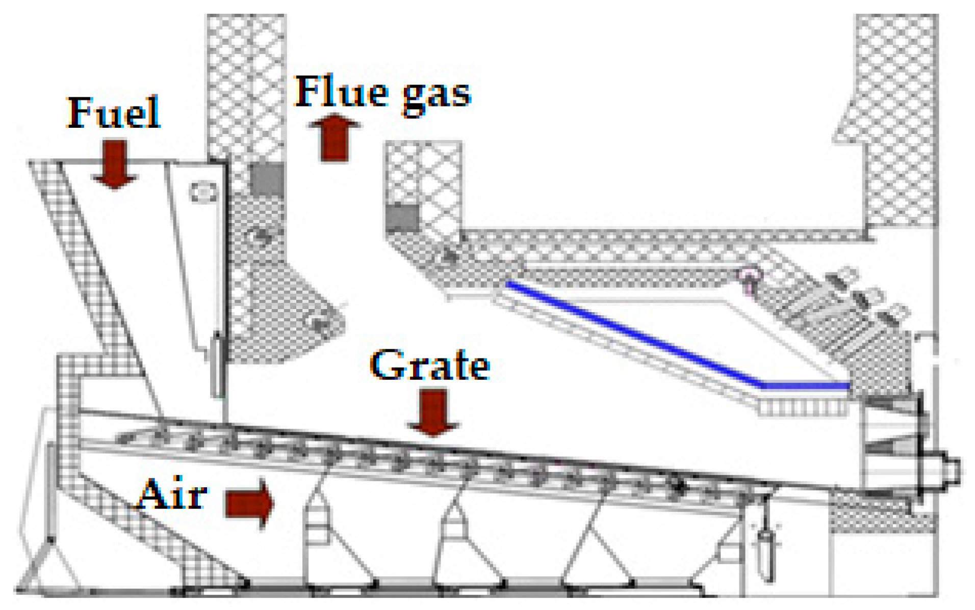
2. Grate Technology in Thermal Treatment of Waste Biomass

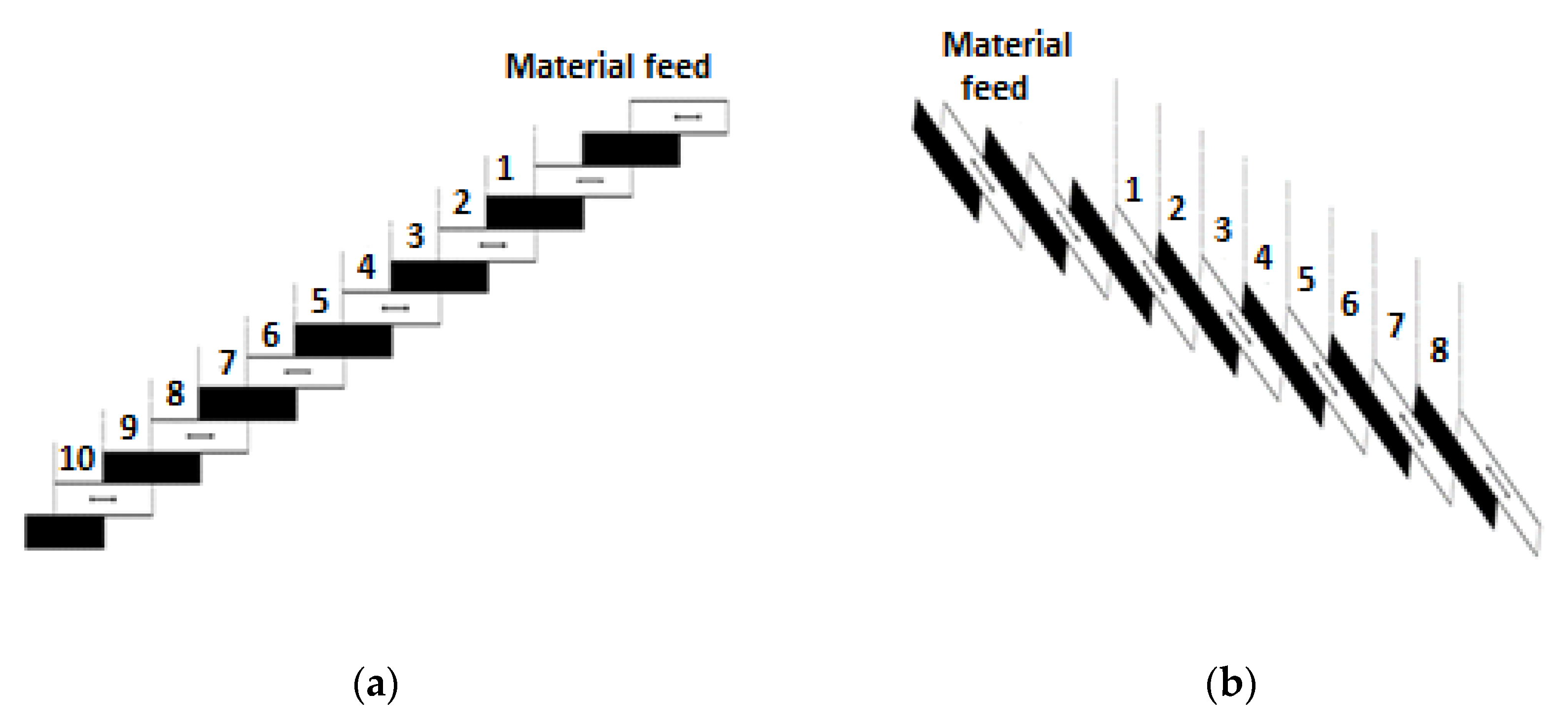
The grate technology used in waste incineration plants enables the transport of waste through the combustion zone as well as intensive mixing and aeration. Ensuring such process conditions is very important for the operation of the incineration plant, as it reduces the possibility of the formation of so-called underfires. These are combustible substances contained in slag and ash. The results of the process are mainly neutralization, a significant reduction of the initial weight and volume of waste, as well as energy recovery [8,9,10].

Figure 1 shows a cross-section through a grate chamber in a waste incinerator.

Each type of grate has to meet certain requirements regarding the supply of primary air under the grate, the possibility of additional cooling, and the speed of movement. The residence time of waste on the grate is usually no more than 60 min. Of the many grate types, the most commonly used in waste management are moving and reciprocating grates [1,17]. They are the subject of the research described in this paper.

2.1. Moving Grate

In moving grates, material is transported toward the slag hopper by the movement of alternating fixed and moving grates. At the same time, this grate can operate in a horizontal or angled arrangement. In an angled arrangement, the grate takes on a stepped form. The feed rate of the grates forces local mixing and regrinding of the material. The moving grates have varieties, which include counter-rotating, stepped, and fluidized-assisted grates. In the case of these grates, the shape of the grates and the supply of primary air should make it possible to reduce to a minimum the amount of fine fraction sifted under the grate. In addition, they should ensure not only the legally required quality of slag and bottom ash but also the regular distribution of primary air over the entire surface of the grate [18,19]. Figure 2 shows the construction of the moving grate in terms of the arrangement of the grates.

2.2. Reciprocating Grate

The reciprocating grates are similar in construction to the moving grates, with the difference consisting of the changed angle of the grates—here it is offset by 90°. The grates make a reciprocating motion in the direction opposite to the slope of the grate, allowing very intensive mixing of the waste material, and a statistical particle repeatedly makes a movement up and down the grate before it is discharged into the slag hopper. This type of grate is particularly popular because of its reliability and very good technical performance. The quality of waste firing is very high. This grate consists of stepped grates in sections spanning the width of the furnace. Appropriate movements of the grates ensure the required level of mixing of the waste and cleaning of the gaps supplying air for the combustion process (primary air, which also acts as a cooling agent for the grate). The movement of the grates in the direction opposite to the movement of the waste allows the formation of a uniform layer of waste and carries some of the incandescent mass drying and igniting the newly delivered waste to the top of the grate. There are many variations of this type of grates with additional moving sections and other combinations [1,3,17]. Figure 3 shows the construction of the reciprocating grate in terms of the arrangement of the grates.

3. Materials and Methods

The study of the movement properties of a bed-solid material on selected types of grates was performed on a laboratory stand designed using the impulse (tracer) method. Several types of solid materials with different rheological properties were selected for testing. Variants of the tests were determined. For each set of parameters, tests were carried out in at least 3 repetitions on a condition reflecting the operation of a combustion chamber equipped with moving and reciprocating grates. Only physical conversions are included in the study.

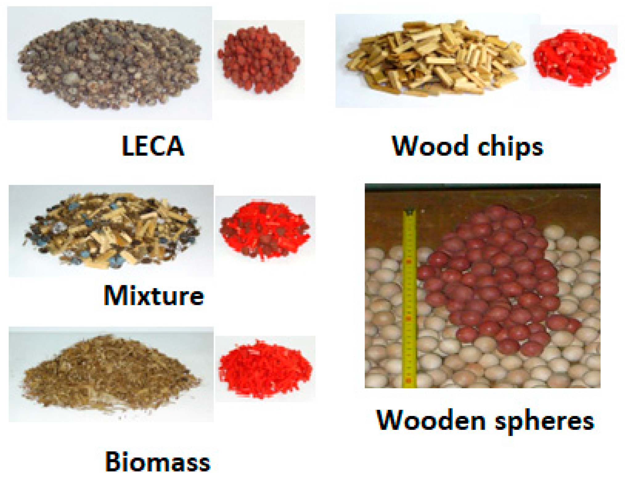
3.1. Properties of the Tested Materials

Tests were conducted for the following materials:

• LECA—lightweight expanded clay aggregate; an artificial porous aggregate obtained by firing formed from clay granules, used as an insulating fill. The study used multifractional expanded clay composed of the following fractions:
  • with a diameter of 10–13 mm—the smallest fraction (uncolored),
  • with a diameter of 13–17 mm—medium fraction (colored blue),
  • with a diameter of 17–20 mm—the largest fraction (colored white).

These fractions were mixed with a mass ratio of: 2:2:1,

• wood chips—wood waste with a length of 40 mm and a thickness of 5 mm,
• biomass-shredded and air-dried green mass (branches + grass) of 50 mm × 2 mm, the mass proportion of grass to branches was: 1:5,
• mixture-LECA + wood chips + biomass mixed in mass ratio of 5:3:1,
• wood spheres with a diameter of 20 and 32 mm.

The selection of the materials studied was not random. Selected properties of materials such as bulk density, apparent density, grain size and shape, as well as porosity, identify (to some extent) the transformation of waste material properties during its combustion on the grate. Biomass (raw waste) was chosen as the input material. The mixture simulates the waste during the process, while the output material (ash, slag) was simulated using expanded clay of varying granulometry.

The markers for the tested materials were prepared by coloring their separated portions.

Table 1. Selected properties of the tested materials.

Parameter	Unit	LECA	Wood Chips	Biomass	Mixture	Wooden Spheres 1	Wooden Spheres 2
Bulk density	kg/m3	290	214	104	208	340	300
Apparent density	kg/m3	664	630	157	549	600	600
Porosity	-	0.55	0.66	0.33	0.62	0.43	0.50
Angle of repose	°	36	43	48	35	-	-
Size	mm	10–20	40 × 5	50 × 2	-	20	32

summarizes selected physical properties of the materials used in the study.

3.2. The Laboratory Stand

The most commonly used grate systems are studied, namely:

• moving grate,
• reciprocating grate.

The tests were carried out without the participation of chemical reactions or heat and mass exchange processes. It was therefore only possible to simulate the physical properties of the tested materials. Two laboratory stands were developed: a moving grate and a reciprocating grate.

The test stand provides regulation of the grates speed and smooth feed. It consists of seven fixed and six moving grate bars. The construction and operation parameters are listed below.

Structural parameters of the grate stand:

• width of a grate: 0.8 m,
• length of a grate bar: 0.37 m,
• surface of a grate: 4144 m².

Operating parameters of the grate:

• range of the feed length: 1–230 mm,
• range of the grate bars velocity: 0–10 mm/s,
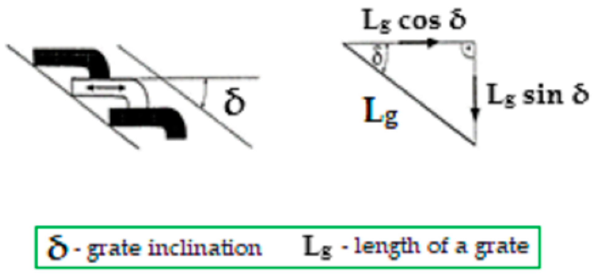
• range of the angle of inclination: 0–30°.

Figure 4 shows the laboratory stands.

Figure 5 schematically shows the places of feeding and collecting the material on the tested types of grates.

The scope of the multi-variant tests carried out included the selection of a couple process variables and their values, as well as the analysis of the impact of the changed parameters on the material flow on the grates. The following variables have been selected:

-

angle of inclination of the grate,

-

grate bars speed,

-

type of feed material (variation of rheological properties),

-

stream of the input material.

Table 2. Tests variants for the moving grate.

Material	Grate Feed Speed [mm/s]	Angle of Inclination [°]	Length of the Grate [m]
LECA	0.5–7	9–16	2.75
Wood chips	0.5–7	9–16	2.75
Biomass	0.5–7	9–16	2.75
Mixture	0.5–7	9–16	2.75
Wooden spheres	0.5–7	9–16	2.75

and

Table 3. Tests variants for the reciprocating grate.

Material	Grate Feed Speed [mm/s]	Angle of Inclination [°]	Length of the Grate [m]
LECA	0.5–7	20–30	2.75
Wood chips	0.5–7	20–30	2.75
Biomass	0.5–7	20–30	2.75
Mixture	0.5–7	20–30	2.75
Wooden spheres	0.5–7	20–30	2.75

list the values of process variables for individual test variants.

3.3. The Course of the Research with the Use of the Impulse Method

In order to determine selected material motion parameters—residence time, mixing intensity, and degree of dispersion—the experimental signal-response method, also known as the impulse method, is used. The role of a signal is usually performed by a properly selected indicator substance (also called a marker or tracer), the specified amount of which is introduced in a strictly defined manner to the stream at the inlet to the grate chamber. The tracer must not react in any way with the stream components. Registration of the concentration of this substance as a function of time at the outlet from the grate makes it possible to determine the distribution function of the residence time of the material on the grate [20,21]. Figure 6 shows the tested materials and their markers.

The determination of the residence time distribution consisted of several steps:

• loading a portion of the material onto the movable grate, stabilizing and establishing a continuous flow on the grate,
• introducing the tracer,
• continuing the introduction of material on the grate to ensure a steady flow on the grate until the last portion of the tracer is received,
• receiving subsequent portions of the material with the tracer (at fixed time intervals) at the outlet of the grate,
• weighing of the tracer in the received portions.
• At the same time, portions of material were collected at specific, fixed time intervals. The tracer was introduced in a very short time, in the entire cross-section filled along the width of the grate, in the form of an impulse signal, and its measurement was carried out in the output stream of the material. For each portion, the mass fraction of the tracer to the mass of the entire portion was determined. These data were transferred to a computational program based on the algorithm presented in the next chapter.

The study of the degree of mixing and dispersion was formulated as the implementation of the following tasks:

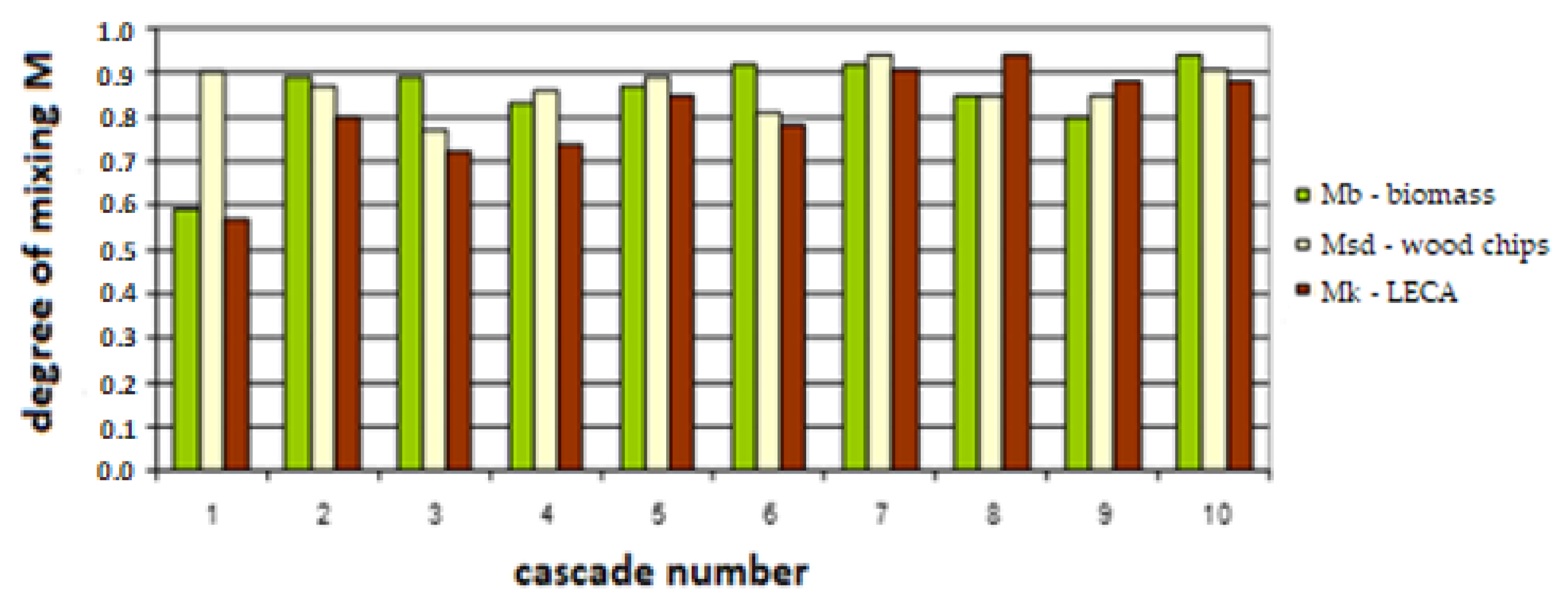
• determination of the degree of mixing materials on the grate,
• determination of the longitudinal mixing on grates,
• recognition and determination of the transverse mixing on grates,
• determination of the degree of dispersion.
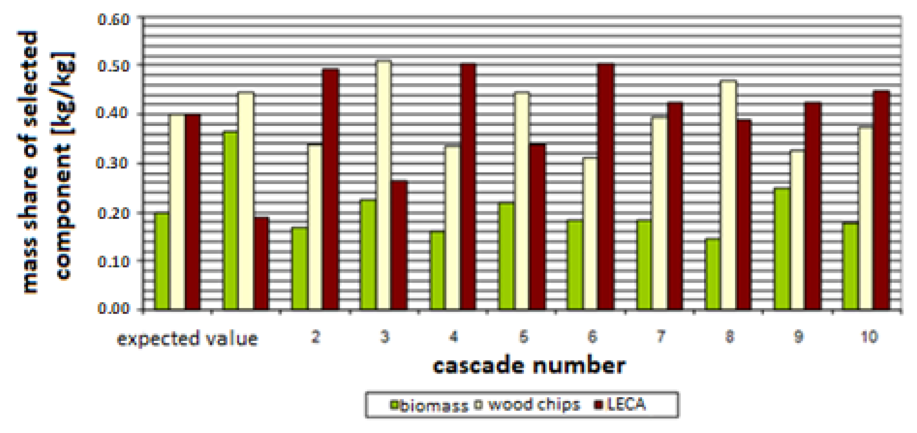
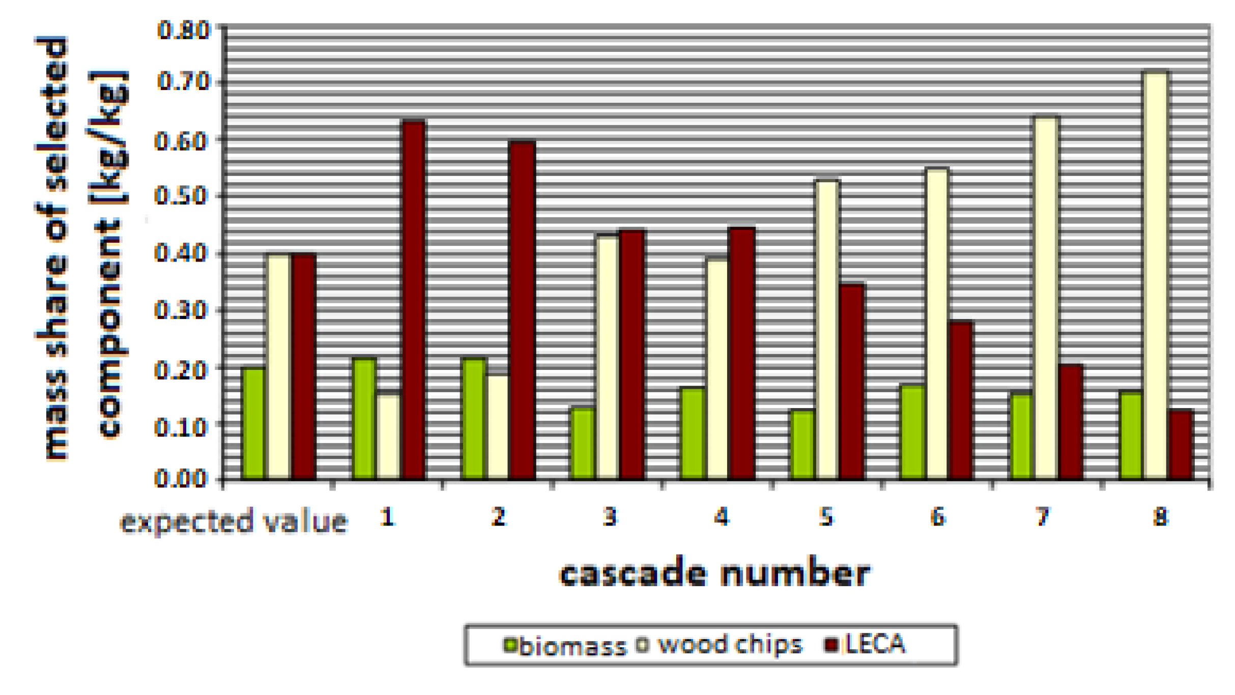
• The degree of mixing of the material on the grate was determined as follows. Each grate, along with its portion of material, was separated from the others by means of two perpendicularly introduced profiled plexiglass plates, thus obtaining the so-called cascades. Each cascade was divided into five equal parts. From each part of the cascade, the material that remained in them was selected, and the mass fractions of individual components were determined. The results were then averaged over the entire cascade. The division diagram is shown in Figure 7.

The materials were introduced in a state of complete segregation in the following order: LECA, biomass, and wood chips. The weights of the introduced portions of material were strictly defined:

• mass of LECA m_k = 2 kg (1.6 kg fraction 10–17 mm, 0.4 kg fraction 17–20 mm),
• mass of biomass m_b = 1 kg, fraction 1 do 40 mm,
• mass of wood chips m_śd = 2 kg, fraction 25 mm.

After the time, which corresponded to the average residence time of the material on the grate, the grate was stopped to collect samples for analysis. Each sample taken was separated and accurately weighed. The mass shares of individual components of the transported material in the cascades formed by grate bars were determined.

4. Model of Residence Time Distribution, Mixing, and Degree of Dispersion

4.1. Introduction to the Algorithm

Algorithms are used on a large scale in technological processes, where their application contributes, among others, to the synchronization and stabilization of the system [22,23]. In case of the modeling of material motion on grates, there are different approaches to this issue in the literature. The analysis of the essential characteristics of the movement of the material on the grates can be performed by adapting the universal theory of flows described, among others, in refs. [6,20,24]. Within the theory, two cases of flow are distinguished: with perfect mixing and piston flow.

In a grate furnace, we deal with a dispersion flow of an unspecified nature, differing to a greater or lesser extent from ideal models. For practical reasons, it is important to assess the degree of approximation to the ideal state. The criterion for such an assessment is provided by two distribution functions of the real residence time of particles:

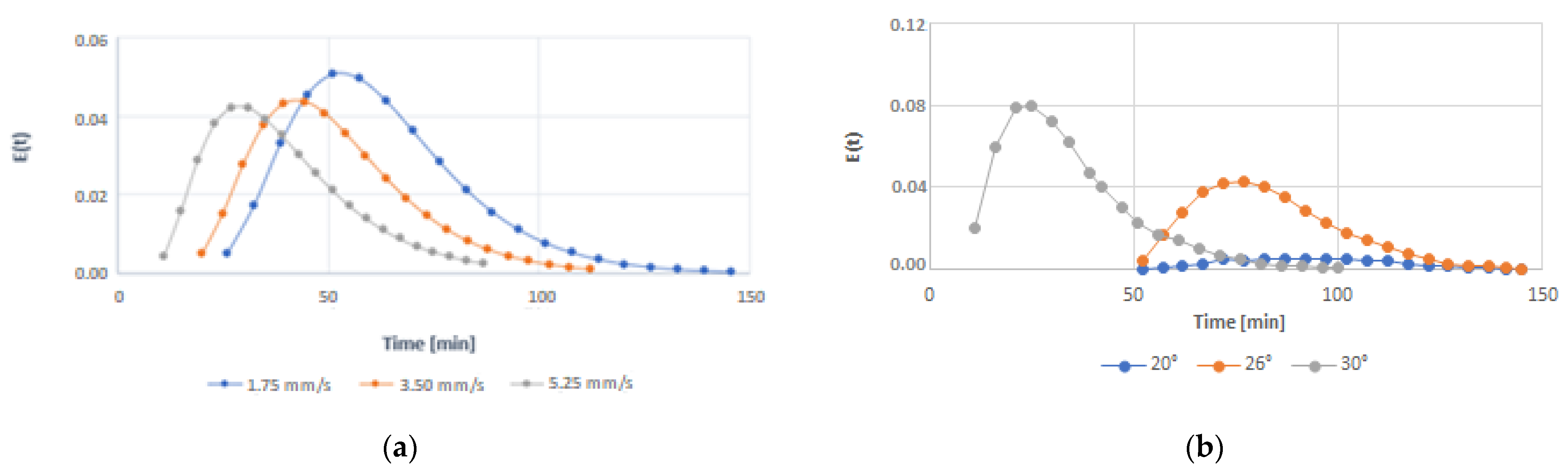
• E(t) specifying the molar (mass) fraction of particles with a residence time within a certain range in the stream leaving the device,
• F(t) the distribution function of the residence time distribution, also called the residence time distribution.

Both functions are the criteria for the previously mentioned compliance of the calculation results with the practical data. Residence time distribution curves are the only objective image of flow dynamics in real conditions.

For the residence time distribution function defined in this way, the following applies:

$${{\displaystyle \int }}_0^{\infty }E\left(t\right)dt=1$$

(1)

The value of the function F(t) for time t provides the part of the stream of particles leaving the grate with a residence time in the range from 0 to t. The relationship between the two functions, resulting from the definition, is as follows:

$$F\left(t\right)={{\displaystyle \int }}_0^{t}E\left(t\right)dt$$

(2)

It follows that:

$$\frac{dF\left(t\right)}{dt}=E\left(t\right)$$

(3)

Moments of these distributions are very helpful in characterizing and comparing residence time distributions. Typically, we use a first moment and a second central moment, called the variance, to evaluate the residence time distribution.

The first moment equals the average residence time:

$$\overline{t}={{\displaystyle \int }}_0^{\infty }tE\left(t\right)dt$$

(4)

The variance characterizes the dispersion of the residence time relative to the mean value:

$${\sigma }_t^2={{\displaystyle \int }}_0^{\infty }\left(t-\overline{t}{)}^{2}E\left(t\right)dt={{\displaystyle \int }}_0^{\infty }{t}^{2}E\left(t\right)dt-{\overline{t}}^{ 2}\right.$$

(5)

The first and second moments of the random variable t uniquely characterize the residence time distribution. In practice, they are used as convenient criteria for comparing the distribution curves. For comparative purposes, it is more advantageous to use dimensionless time, related to the average residence time of the material on grates:

$$\theta =\frac{t}{\overline{t}}$$

(6)

This parameter is called the relative residence time. It is also a random variable with the same distribution functions as t.

$$F\left(\theta \right)=F\left(t\right)$$

(7)

$$E\left(\theta \right)=\overline{t}E\left(t\right)$$

(8)

Using dimensionless time, the moments and width of the distribution curve can be represented as follows:

$$\overline{t}={{\displaystyle \int }}_0^{\infty }\theta E\left(\theta \right)d\theta =1$$

(9)

$${\sigma }_{\theta }^2=\frac{{\sigma }_t^2}{{\overline{t}}^2}={{\displaystyle \int }}_0^{\infty }\left(\theta -1{)}^{2}E\left(\theta \right)d\theta ={{\displaystyle \int }}_0^{\infty }{\theta }^{2}E\left(\theta \right)d\theta -1\right.$$

(10)

An important issue here is the interpretation of the response curves in real reactors and their connection with the Peclet number given by the formula:

$$P{e}_L=\frac{uL}{D_L}$$

(11)

where:

• L—reactor length, [m],
• u—linear speed, [m/s],
• $D_L$—longitudinal dispersion coefficient, [m²/s].

The $D_L$ coefficient is an effective substitute value (constant in the cross-section), which allows us to capture the mixing phenomena along the reactor axis in a uniform manner, regardless of their nature.

The value of $P{e}_L$ characterizes the flow dynamics and is a measure of the intensity of longitudinal mixing in the reactor. The shape of the residence time distribution curves E(t) and F(t) depends on their values. For borderline cases, it takes the following value:

$P{e}_{L }$= 0 ($D_L$ = ∞)—perfect mixing (tank reactor),

$P{e}_L$= ∞ ($D_L$ = 0)—no mixing (tube reactor).

A flow in which the mixing phenomenon can be described by the number $P{e}_L$ or the coefficient $D_L$ and there is no variation of concentrations in the cross-section of the stream is called dispersion flow.

Depending on the assumed boundary conditions in the considered case, various models of dispersion flow are obtained, binding the distribution functions E(θ) or F(θ) and their parameters ${\sigma }_{\theta }^2$, $\overline{\theta }$ with the Peclet number. Theoretically determined dependences of variance on the Peclet number are of the greatest importance. If the variance ${\sigma }_t^2$ or ${\sigma }_{\theta }^2$ is determined from the experimental curves E(θ), then using the appropriate equation of boundary conditions, it is possible to estimate the value of the number $P{e}_L$. The Peclet number found in this way is a measure of the average dispersion in the working zone of the device (between the signal input and output points).

With regard to the grate reactor, in which the flow is dispersive D/uL > 0.01, and for the boundary conditions of the “open vessel”, the residence time spectrum in the mathematical notation is expressed by the equation:

$$E\left(t\right)=\frac{u}{\sqrt{4\pi tD}}exp\left[-\frac{{(L-ut)}^2}{4tD}\right]$$

(12)

or in dimensionless form:

$$E\left(\theta \right)=\frac{1}{\sqrt{\left(4\pi \Theta P{e}_L^{-1}\right)}}exp\left[-\frac{{(1-\Theta )}^2}{4\Theta P{e}_L^{-1}}\right]$$

(13)

On the basis of the above general relationships, an algorithm dedicated to determining the residence time distribution (RTD), mixing, and degree of dispersion is developed.

4.2. Algorithm for the RTD, Mixing, and Degree of Dispersion Calculation

Bearing in mind the lack of knowledge of the values that allow the calculation of the $P{e}_L$, the analytical form of the above equation can be presented (by introducing independent parameters: “α” i “b”) in the form:

$$E\left(\theta \right)=\mathsf{\alpha }{\theta }^{-0.5}exp\left[b\frac{{(1-\Theta )}^2}{\Theta }\right]$$

(14)

The regression function is used to develop the results of the measurement of the RTD. In this case, to estimate the structural parameters of the regression curve, as reported in refs. [5,21], the least squares method can be used if the function is reduced as follows:

$$\ln E\left(\theta \right)=\ln \alpha -0.5\ln \Theta +b\frac{{(1-\Theta )}^2}{\Theta }$$

(15)

In addition, by introducing simplifying notations:

$$z=\ln E\left(\theta \right)$$

(16)

$$x=\ln \theta$$

(17)

$$y=\frac{{(1-\Theta )}^2}{\Theta }$$

(18)

$$z=\alpha -0.5x+by$$

(19)

Estimating the structural parameters of the regression function is achieved by finding the minimum expression:

$$W=\sum {(z_i-\ln M_i)}^2$$

(20)

$$W=\sum {(\alpha -0.5x_i+b{y}_i-\ln M_i)}^2$$

(21)

For data from the “m” sample, values ($M_i, {\theta }_i$), i = 1, …, m, where: m—number of measurement, $M_i$—relative mass of the received tracer (calculated relative to the initial mass of the inserted tracer $m_o$), expressed by the equation:

$$M_i=\frac{m_i}{m_0}$$

(22)

Since the equation is a function of two variables α i b, the issue comes down to finding the minimum of a quadratic function of two variables. A necessary condition for the existence of an extremum is the zeroing of partial derivatives.

$$\frac{\delta W}{\delta \alpha }=0$$

(23)

$$\frac{\delta W}{\delta b}=0$$

(24)

As a result of the differentiation of the function defined by the equation by variables α and b, a system of two linear equations is obtained. Since time here is dimensionless with respect to the average residence time $t_m$, it is necessary to find a third equation that is a function of only three parameters: α, b oraz $t_m$. This is achieved by assuming an additional condition that determines how the solution is obtained, thus:

• Variant 1: Assumes that the sum of the relative measured masses $M_i$ is equal to the sum of the values determined by the regression function E(${\theta }_i$), which is expressed by the following equation:

  $$\sum M_i=\sum E\left({\theta }_i\right)\hspace{1em}\hspace{1em}\mathrm{for}i=1,\dots ,m$$

  (25)

• Variant 2: Assumption that the sum of the values determined by the regression function E(${\Theta }_j$) is a consequence of the relative notation: mass of the received tracer and residence time. Therefore, this algorithm takes into account the following condition:

  $$E\left({\theta }_j\right)=1\hspace{1em}\hspace{1em}\mathrm{for}i=1,\dots ,n,$$

  (26)

  where: n—the number of values of E(θ_j) determined by the regression function.

• Variant 3: The combination of the conditions presented above is the assumption.

Calculations of numerical values of unknown parameters (α, b oraz $t_m$) are made by the program taking into account the following three conditions:

$$\frac{\delta W}{\delta \alpha }=0 \Rightarrow t_m$$

(27)

$$\frac{\delta W}{\delta b}=0 \Rightarrow b$$

(28)

And

-

for the variant 1 ⇒ α (a)

$$a=\frac{\sum M_i}{\sum {\Theta }_i^{-0.5}{e}^{b{y}_i}}$$

(29)

-

for the variant 2 ⇒ α (a)

$$a=\frac{1}{\sum {\Theta }_i^{-0.5}+e^{b{y}_i}}$$

(30)

-

for the variant 3 ⇒ α (a)

$$a=\frac{1+\sum M_i}{\sum {\Theta }_i^{-0.5}{e}^{b{y}_i}+\sum {\Theta }_i^{-0.5}{e}^{b{y}_i}}$$

(31)

To calculate the value of the average residence time of the materials in the rotating cylinder, the computer program uses the iteration method, for which it sets the parameters: the maximum number of iterations and the maximum change to 500 and 10⁻⁶, respectively. This makes it possible to achieve high accuracy in the solution generated by the program in a relatively short time.

The expression of the dispersion of the residence time of the material on the grate systems in relation to its average value is the variance. In the case of an impulse stimulus, the formula in which the variance is defined as:

$${\sigma }_t^2=\frac{\sum t_i^{2}E\left(t_i\right)\Delta t_i}{\sum E\left(t_i\right)\Delta t_i}+t_m^2$$

(32)

Also considering that for an open system, the equality is true:

$$\frac{{\sigma }_t^2}{t_m^2}=\frac{2}{P{e}_L^2}\left(P{e}_L+4\right)$$

(33)

the value of the Peclet number can be determined, which, being a description of the degree of mixing intensity, will classify the tested flow as a flow with low, medium, or high mixing, and thus decide on the correctness of the calculations. If the condition $P{e}_L^{-1}$ > 0.01 is not met (this will happen when the mixing of the material in the rotary kiln is small), the average residence time of the material in the kiln can be calculated, according to Levenspiel in ref. [6], straight from the equation:

$$t_m=\frac{\sum t_i{c}_i\Delta t_i}{\sum c_i\Delta t_i}$$

(34)

where:

$t_i$—the time from when the tracer is inserted to when it is received, [s],

$\Delta t_i$—the time interval for the collection of individual portions of the material, [s],

$c_i$—tracer concentration (the share of tracer weight in a given portion to the weight of the entire tracer), [kg/kg].

The determination of the diffusion value of the Peclet number is, in the case of a large mixing of the material in the furnace, the last operation performed by the developed algorithm.

The degree of mixing has been specified in relation to the key component. It is the component whose share determines the quality of the mixture. The remaining components are considered together as the “second component”. It was assumed that the expected mixture should correspond to the condition that, after mixing, the mass fractions of individual components will correspond to the ratio in which they were introduced in the state of segregation. In the conducted tests, the values of the degree of mixing were calculated for three variants of key components, respectively:

• key component—wood chips—expected value p = 0.4,
• key component—LECA—expected value p = 0.4,
• key component—biomass—expected value p = 0.2.

The value of the degree of mixing on individual grate bars is calculated using the Rose formula [2,3]:

$$M=1-\frac{\sigma }{{\sigma }_0}$$

(35)

The standard deviation in the state of primary segregation is calculated from the equation:

$${\sigma }_0={\left[p_0\left(1-p_0\right)\right]}^2$$

(36)

The standard deviation of the tests is expressed by the formula:

$$\sigma =\sqrt{\frac{{{\displaystyle \sum }}_{i=1}^n{(x_i-p)}^2}{n}}$$

(37)

where: x_i—mass fraction of the key component in the sample taken,

p—expected value of the key component,

n—number of samples taken (n = 5 for each cascade).

Dispersive mass transport on the analyzed grates can be described by equations that allow to determine the concentration field in a one-dimensional (x) or two-dimensional (x,y) coordinate system depending on time (t):

$$\frac{\partial c\left(x,t\right)}{\partial t}=D_L\frac{{\partial }^{2}c\left(x,t\right)}{\partial x^2}-u\left(x,t\right)\frac{\partial c\left(x,t\right)}{\partial x}$$

(38)

$$\frac{\partial c\left(x,y,t\right)}{\partial t}=D_L\frac{{\partial }^{2}c\left(x,y,t\right)}{\partial x^2}+D_p\frac{{\partial }^{2}c\left(x,y,t\right)}{\partial y^2}$$

(39)

The choice of the equation depends on the assumption of the presence or absence of transport in the direction transverse to the main direction. The diffusion coefficients in the longitudinal D_L and transverse D_P directions contained in the equations in the conditions of waste mass flow, not liquids, on the analyzed grate systems are determined as longitudinal and transverse dispersion coefficients.

In order to determine the dependencies allowing the calculation of the longitudinal and transverse dispersion coefficients on the analyzed grate systems, a dimensional analysis is used [25,26]. Previously, the dependence of these coefficients on various parameters and quantities, which then formed the basis for the dimensional analysis, was checked.

In order to determine the longitudinal dispersion coefficient D_L the formula defining the Peclet number Pe_L was used.

$$D_{LR}=\frac{u_m{L}_R}{P{e}_L}$$

(40)

where:

L_R—length of the grate [m],

u_m—average speed of the waste material on the grate [m/s],

$$u_m=\frac{L_R}{t_{śr}}$$

(41)

To facilitate the calculation of the longitudinal dispersion coefficient of the material on the grate, a formula was developed to calculate the so-called theoretical longitudinal dispersion coefficient D_LT based on dimensional analysis. It is assumed that D_LT depends on the following parameters: grate velocity (u_R), particle diameter (d_p), material bulk density (ρ_n) on the grate, mass flow rate (m):

$$D_{LT}=f\left(u_R,d_p,{\rho }_n,m\right)$$

(42)

In the first step, an equation connecting these quantities is created:

$$D_{LT}=C{u}_R^A d_p^{B }{\rho }_n^D m^E$$

(43)

This equation is written in accordance with the principles of dimensional analysis, i.e., according to units. It is also assumed that the longitudinal dispersion coefficient decreases with an increase in grain diameter. The equation obtained is:

$$D_{LT}=C{u}_R^0 d_p^{-1} {\rho }_n^{-1} m^1$$

(44)

Eventually, this equation took the form:

$$D_{LT}=C\frac{m}{d_{p }{\rho }_n}$$

(45)

The following forms of equations for longitudinal dispersion coefficients have been proposed for layers:

(a)

monodisperse

$$D_{LT}=C\frac{m}{d_{p }{\rho }_n}$$

(46)

(b)

polydisperse:

$$D_{LT}=C\dot{m}{\displaystyle \sum }_i\frac{1}{d_{pi} {\rho }_{ni}}$$

(47)

where:

D_LT—theoretical longitudinal dispersion coefficient on the grate [m²/s],

d_p—equivalent diameter of the waste material [m],

ρ_n—bulk density of the waste material [kg/m³],

m—mass flow rate of the waste material [kg/s],

C—constant in equations.

The term $\frac{m}{d_{p }{\rho }_n}$ has been replaced with “W”:

$$\frac{m}{d_{p }{\rho }_n}=W$$

(48)

$$D_{LR}=CW$$

(49)

From the equation above, one can obtain:

$$C=\frac{D_{LR}}{\mathrm{W}}$$

(50)

Furthermore, in order to obtain the average value of the constant C, on the basis of the test results and the values obtained using the program, trend lines (regression) were developed for a specific grate inclination angle.

5. Results and Discussion

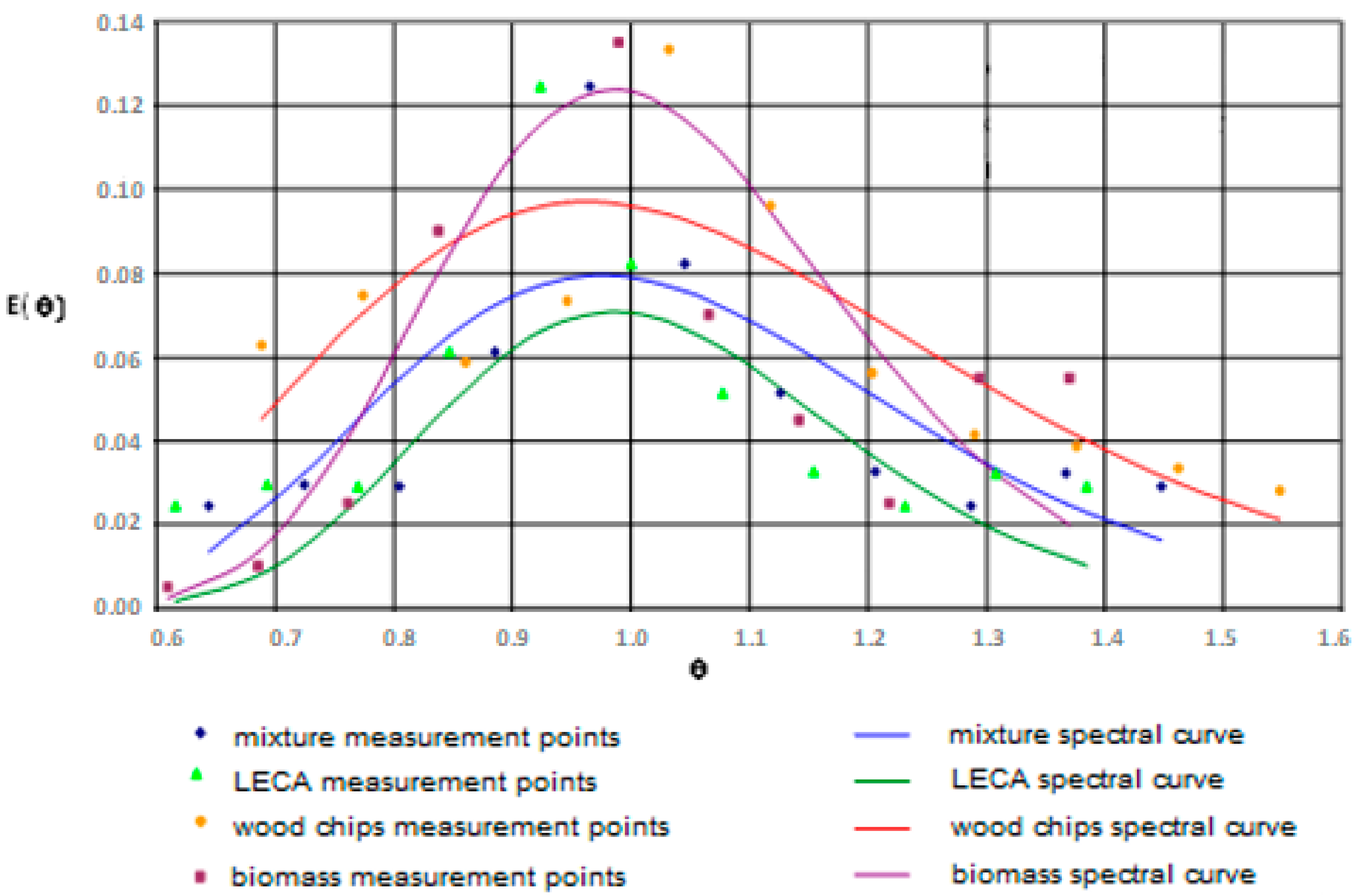
5.1. Residence Time Distribution

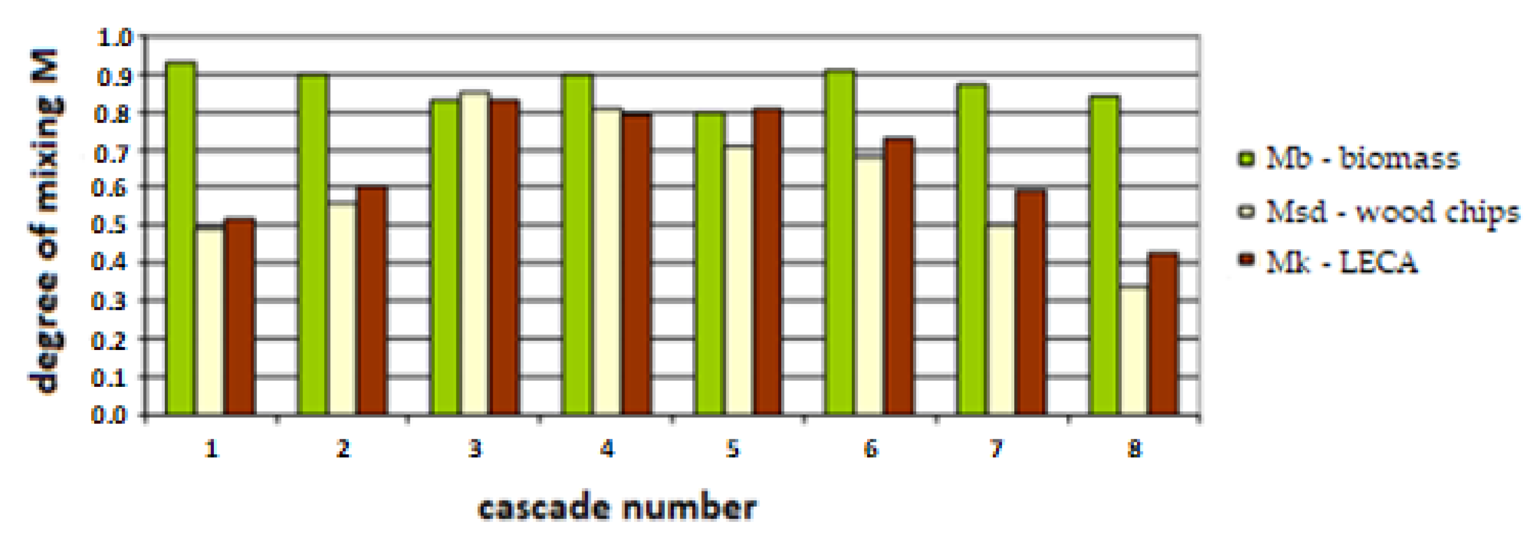
The influence of individual variables on the residence time distribution of the material on the grate is shown in Figure 8, Figure 9, Figure 10 and Figure 11.

The influence of the velocity of the grate bars and the angle of inclination of the grate on the average residence time of the material on the grate can be noticed. This influence is visible to the smallest extent in the case of changes in the angle of inclination of the grate in the case of a moving grate. A general relationship observed is that for angles smaller than 20°, the transport of all tested materials (regardless of the velocity of the grate bars) was only up the grate, so it had no practical significance. At an inclination angle of 30°, very short residence times were obtained, as can be seen in the example of the reciprocating grate. In this case, the angle of natural repose of the material (close to the angle of inclination of the grate) had a larger impact on the velocity of transport than the mechanisms of forced transport on the grate.

In the case of the sliding grate, the distribution of the marker material was U-shaped. A small effect of the grate inclination angle on the average time of material residence on the grate can be noticed, the velocity of the grate bars has a greater impact.

The residence time distribution of the tested materials on the reciprocating grate is shown in Figure 11.

The graph in Figure 10 for material with different granulation (but with the same density) shows the tendency for the largest grains to leave the grate faster (shorter RTD and higher values of the E($\theta$) function). The increase in the velocity of the grate bars maintains this tendency. The graph shows the effect of material particle size on residence time: larger particles have shorter average residence times. Granular material with a constant apparent density but with different granulation, in the case of the reciprocating grate, also tends to have shorter residence times of the largest grains; however, the distribution function E($\theta$) representing the mass fraction of the material collected in the average residence time is many times smaller than it was in the case of a moving grate.

For all the tested materials, the polydisperse material was separated on the grate in a characteristic way. The fine fraction was located in the upper part of the grate and the coarse fraction in the lower part. Shorter residence times of fractions with a larger grain size were found. The rule was to push the coarse fraction onto the surface of the layer before the fine fraction. For all combinations of grate inclination angle and grate velocity, the biomass tended to pile up and “wave”. There were “hinges” and free spaces.

The average residence time, determined according to the algorithm presented in the study on the basis of the experimental results, shows that in both cases of moving and reciprocating grates, the material stays on the grate for a shorter period with increasing velocity of the grate bars.

5.2. Mixing

The obtained values of the degree of mixing M for selected variants of the key component for the moving and reciprocating grate are summarized in

Table 4. Values of the degree of mixing for the moving grate.

Cascade Number	Degree of Mixing Relative to the Selected Key Component M
	Wood Chips Msd	LECA, Mk	Biomass, Mb
1	0.90	0.57	0.59
2	0.87	0.80	0.89
3	0.77	0.72	0.89
4	0.86	0.74	0.83
5	0.89	0.85	0.87
6	0.81	0.78	0.92
7	0.94	0.91	0.92
8	0.85	0.94	0.85
9	0.85	0.88	0.80
10	0.91	0.88	0.94

and

Table 5. Values of the degree of mixing for the reciprocating grate.

Cascade Number	Degree of Mixing Relative to the Selected Key Component M
	Wood Chips Mśd	Keramzyt, Mk	Biomasa, Mb
1	0.49	0.52	0.93
2	0.56	0.60	0.90
3	0.85	0.83	0.83
4	0.81	0.79	0.90
5	0.71	0.81	0.80
6	0.68	0.73	0.91
7	0.50	0.59	0.87
8	0.34	0.43	0.84

.

For the moving grate, the values of the degree of mixing M in individual cascades were similar and reached high values.

A graphic interpretation of the mixing degree of successive cascades for selected grate types is shown in Figure 12 and Figure 13.

For the moving grate, the mixture along the entire length of the grate has a similar composition (flow similar to piston flow). The values of the degree of mixing M in individual cascades are close to each other. The obtained values are related to the method of loading in the state of segregation-successively individual components with a piston flow character (Pe = 300). Mixing takes place over a short distance between the transported components; hence, the mixture along the entire length of the grate has a similar composition.

The values of the degree of mixing M in individual cascades for the reciprocating grate are listed in Table 5.

Graphical interpretation of the mixing degree of successive cascades for selected grate types is shown in Figure 14 and Figure 15.

For the reciprocating grate, the mixing degree values vary over a wide range. High values were obtained for the transported material located in the middle of the length of the grate. At the inlet and outlet of the grate, the mixing ratios are low due to the segregation of the components that accompanies the transport of the material. Smaller particles are transported up the grate, while larger particles tend to be transported faster. Hence, the size of the particles determines the speed of transport more than the difference in their density.

In the case of the reciprocating grate, the values of the degree of mixing vary over a wide range. Only from the point of view of biomass as a key ingredient, the discrepancy ranges from 0.84 to 0.93. In the case of wood chips, the value of Msd varies from 0.49 for 1 cascade and then reaches high values for 3 and 4 cascades, 0.85 and 0.81, respectively. However, for successive cascades, it assumes lower and lower values. The situation is similar for the LECA component. This is due to the segregation of components along the length of the grate, which is accompanied by intensive longitudinal mixing, which is shown in the graph of mass shares in the cascades. LECA grains are transported up the grate, while wood chips tend to be transported faster along the length. The numerical value M itself does not capture this phenomenon. It only specifies a deviation from the expected composition but does not specify the cause—whether it is caused by an excess or deficiency of the selected component. A perfect example of the discussed phenomenon is the comparison of the Mk values for cascade numbers 2 and 7. The Mk values are Mk = 0.60 and Mk = 0.59, respectively, while the shares of expanded clay are 0.60 and 0.21.

5.3. Degree of Dispersion

Table 6. Moving grate, LECA 10–20 mm.

Angle of Inclination	Grate Bar Velocity	Mean Residence Time	Mean Material Velocity	Pe	W	C	Mean C	DLR	DLT	Relative Error
[°]	[mm/s]	[min]	[m/s]	[-]	[m2/s] ∙103	[-]	[-]	[m2/s] ∙103	[m2/s] ∙103	[%]
9	1.5	53.29	0.0009	46	1.726	0.030	0.036	0.0525	0.0621	18.2
9	3.5	30.14	0.0015	40	2.416	0.044		0.1068	0.0870	18.6
9	7.0	20.00	0.0023	40	4.629	0.035		0.1610	0.1666	3.5
13	1.5	50.29	0.0012	34	1.874	0.052	0.046	0.0965	0.0862	10.7
13	3.5	26.34	0.0018	39	3.093	0.041		0.1254	0.1423	13.5
13	7.0	16.21	0.0029	37	4.584	0.047		0.2148	0.2108	1.8
16	1.5	39.24	0.0009	18	1.893	0.071	0.085	0.1343	0.1609	19.8
16	3.5	25.00	0.0019	19	3.132	0.087		0.2712	0.2663	1.8
16	7.0	15.38	0.0030	20	4.882	0.086		0.4187	0.4150	0.9

,

Table 7. Moving grate, wood spheres 20 mm.

Angle of Inclination	Grate Bar Velocity	Mean Residence Time	Mean Material Velocity	Pe	W	C	Mean C	DLR	DLT	Relative Error
[°]	[mm/s]	[min]	[m/s]	[-]	[m2/s] ∙103	[-]	[-]	[m2/s] ∙103	[m2/s] ∙103	[%]
4	3	84.47	0.0005	36.97	0.283	0.15	0.14	0.0412	0.0396	4.1
4	6	35.21	0.0013	35.77	0.782	0.13		0.1023	0.1094	7.0
4	9	22.96	0.0020	34.60	1.199	0.14		0.1621	0.1678	3.5
8	3	79.97	0.0006	27.93	0.328	0.18	0.24	0.0577	0.0787	36.6
8	6	34.83	0.0013	20.35	0.788	0.23		0.1818	0.1890	4.0
8	9	19.85	0.0023	22.32	1.184	0.25		0.2908	0.2840	2.3
12	3	63.39	0.0007	17.23	0.318	0.37	0.39	0.1179	0.1239	5.1
12	6	26.97	0.0017	15.06	0.735	0.43		0.3170	0.2868	9.5
12	9	17.16	0.0027	17.41	1.159	0.37		0.4312	0.4519	4.8

,

Table 8. Reciprocating grate, LECA 10–20 mm.

Angle of Inclination	Grate Bar Velocity	Mean Residence Time	Mean Material Velocity	Pe	W	C	Mean C	DLR	DLT	Relative Error
[°]	[mm/s]	[min]	[m/s]	[-]	[m2/s] ∙103	[-]	[-]	[m2/s] ∙103	[m2/s] ∙103	[%]
22	3	63.98	0.0007	10.80	0.720	0.23	0.27	0.1967	0.1944	1.2
22	6	32.67	0.0013	13.70	0.960	0.25		0.2870	0.2592	9.7
22	9	24.52	0.0017	11.20	1.410	0.34		0.4120	0.3807	7.6

and

Table 9. Reciprocating grate, wood spheres 20 mm.

Angle of Inclination	Grate Bar Velocity	Mean Residence Time	Mean Material Velocity	Pe	W	C	Mean C	DLR	DLT	Relative Error
[°]	[mm/s]	[min]	[m/s]	[-]	[m2/s] ∙103	[-]	[-]	[m2/s] ∙103	[m2/s] ∙103	[%]
22	3	83.93	0.0006	6.62	0.238	0.97	1.07	0.2319	0.2550	10.0
22	6	44.57	0.0010	7.12	0.401	1.01		0.406	0.4286	5.6
22	9	27.32	0.0017	6.27	0.684	1.10		0.7526	0.7314	2.8
26	3	61.60	0.0008	8.19	0.251	1.02	1.09	0.2553	0.2731	7.0
26	6	34.32	0.0014	9.20	0.430	0.95		0.4081	0.4688	14.9
26	9	21.01	0.0022	7.76	0.685	1.15		0.7899	0.7466	5.5

summarize selected variants of the experimental tests carried out and present a comparative analysis with the results of the calculated longitudinal dispersion coefficients, both real and theoretical. The value of the relative error between these values has been shown. The value of the constant C has also been compiled.

The average value of the relative error determined based on the comparison of the theoretical longitudinal dispersion coefficient to the actual longitudinal dispersion coefficient showed a satisfactory value of 8.26% for the moving grate (error range from 0.9% to 36.6%) and 7.63% for the reciprocating grate (error range from 2.8% to 14.9%).

Knowledge of the value of the constant C provides the possibility to quickly determine the dispersion coefficient without the need to use the RTD program and perform laboratory tests. The given method of determining the constant C for other materials in a variant with operating data will expand the range of possibilities for D_L determination and use in calculations of mass transport on grates in incineration plants.

6. Conclusions

Mass transport of material on moving and reciprocating grates is undoubtedly a complex issue, both from the cognitive side of the physical and chemical phenomena taking place and in terms of mathematical description.

In summary, the following characteristics of the process of material transport on the selected types of grates can be distinguished.

Moving grates:

• low backward mixing,
• short average residence times of materials,
• low layer heights of material on the grate,
• formation of the velocity profile in the form of a “U” (top view).
• Reciprocating grates:
• high degree of mixing of material on the grate,
• long average residence times of the material,
• the material transport mechanism (for grate inclination angle >30°) is more affected by the natural angle of repose of the material than by the movement caused by the mechanical feed of the grate bars,
• for 30°, rapid surface sloughing was observed, without mixing,
• when transporting polydisperse material (different size fractions), separation of small fractions in the upper part of the grate, large fractions in the lower part of the grate was observed.

In modeling the transport of material on the grate, the above information is of great importance in selecting the optimal grate slope, velocity of grate bars, and other parameters in the process of designing or operating the grate. Knowledge enriched by the analysis of the movement and behavior of different fractions of solid material will be invaluable and helpful in modeling the process of combustion of waste materials.

One of the novelties introduced to the modeling of mass flow on grates is the Peclet number parameter. Analyzing the values of this parameter, it can be noticed that the degree of dispersion is mainly influenced for moving and reciprocating grates by the inclination angle of the grate:

• for a moving grate, as the grate inclination angle increases by several degrees, the Peclet number decreases and the dispersion intensity increases,
• for a reciprocating grate, the Peclet number increases with an increase in the angle of inclination; this is due to excessive inclination, when part of the material falls from the grate mainly by gravity (the angle of natural repose of the material is exceeded).

For a moving grate, the degree of mixing M in individual cascades reaches similarly high values. This parameter, introduced by the authors to the methodology of determining the mass flow on different types of grates, increases the possibility of describing the mixing of the material. For a reciprocating grate, the mixing degree values vary over a wide range. High values were obtained for the transported material that stayed in the middle of the grate length. At the inlet and outlet of the grate, the mixing degree values are low due to the segregation of components accompanying the transport of material. Smaller particles are carried up the grate, while larger particles tend to be transported faster. Particle size determines faster transport more than the difference in their density.

Granular material with constant apparent density but varying granularity also shows a tendency for shorter transit times of the largest grains in the case of the reciprocating grate, but the distribution function E($\theta$) representing the mass share of the material received in the average residence time takes on smaller values than it did in the case of the moving grate. Similar tendencies were also noticed by refs. [13,15,27]. In the case of mixing and dispersion, it is possible to compare the longitudinal diffusion coefficient, the value of which was also determined by refs. [13,14,28]. The range of values for stands simulating the operation of real industrial grates is: 18.5–61.5 cm²min⁻¹ [13], 27–109 cm²min⁻¹ [14] and 0.09–24,000 cm²min⁻¹ [28]. The results obtained in this study are in the range of 22–474 cm²min⁻¹. They are in a wide range from the study [28], and in the vast majority, they are consistent with the results [13,14].

References

1. Kozioł, M.; Kozioł, J. Impact of Primary Air Separation in a Grate Furnace on the Resulting Combustion Products. Energies 2023, 16, 1647. [Google Scholar] [CrossRef]
2. Zhuang, J.; Tang, J.; Aljerf, L. Comprehensive review on mechanism analysis and numerical simulation of municipal solid waste incineration process based on mechanical grate. Fuel 2022, 320, 123826. [Google Scholar] [CrossRef]
3. Leckner, B.; Lind, F. Combustion of municipal solid waste in fluidized bed or on grate—A comparison. Waste Manag. 2020, 109, 94–108. [Google Scholar] [CrossRef]
4. Jaworski, T. Investigation on Physicochemical Variations of Waste Substances Properties During Combustion Process in Grate Fired Experimental Incineration System. Waste to Energy and Environment; Helion: Gliwice, Poland, 2010; pp. 127–140. [Google Scholar]
5. Burghardt, A.; Bartelmus, G. Chemical Reaction Engineering. Reactors for Homogeneous Systems; PWN: Warsaw, Poland, 2001. [Google Scholar]
6. Levenspiel, O. Chemical Reaction Engineering, 3rd ed.; John Wiley & Sons: Berlin/Heidelberg, Germany, 1991. [Google Scholar]
7. Jiang, M.; Lai, A.; Law, A. Solid Waste Incineration Modelling for Advanced Moving Grate Incinerators. Sustainability 2020, 12, 8007. [Google Scholar] [CrossRef]
8. Poranek, N.; Łaźniewska-Piekarczyk, B.; Lombardi, L.; Czajkowski, A.; Bogacka, M.; Pikoń, K. Green Deal and Circular Economy of Bottom Ash Waste Management in Building Industry—Alkali (NaOH) Pre-Treatment. Materials 2022, 15, 3487. [Google Scholar] [CrossRef] [PubMed]
9. De Greef, J.; Hoang, Q.N.; Vandevelde, R.; Meynendonckx, W.; Bouchaar, Z.; Granata, G.; Verbeke, M.; Ishteva, M.; Seljak, T.; Van Caneghem, J.; et al. Towards Waste-to-Energy-and-Materials Processes with Advanced Thermochemical Combustion Intelligence in the Circular Economy. Energies 2023, 16, 1644. [Google Scholar] [CrossRef]
10. Poranek, N.; Łaźniewska-Piekarczyk, B.; Czajkowski, A.; Pikoń, K. MSWIBA Formation and Geopolymerisation to Meet the United Nations Sustainable Development Goals (SDGs) and Climate Mitigation. Buildings 2022, 12, 1083. [Google Scholar] [CrossRef]
11. Kruggel-Emden, H.; Kacianauskas, R. Discrete element analysis of experiments on mixing and bulk transport of wood pellets on a forward acting grate in discontinuous operation. Chem. Eng. Sci. 2013, 92, 105–117. [Google Scholar] [CrossRef]
12. El Korchi, K.; Alami, R.; Saadaoui, A.; Mimount, S.; Chaouch, A. Residence time distribution studies using radiotracers in a lab-scale distillation column: Experiments and modeling. Appl. Radiat. Isot. 2019, 154, 108889. [Google Scholar] [CrossRef]
13. Kruggel-Emden, H.; Wirtz, S. Analysis of Residence Time Distributions of Different Solid Biomass Fuels by using Radio Frequency Identification (RFID). Energy Technol. 2014, 2, 498–505. [Google Scholar] [CrossRef]
14. Yang, Y.B.; Lim, C.N.; Goodfellow, J.; Sharifi, V.N.; Swithenbank, J. A diffusion model for particle mixing in a pecked bed of burning solids. Fuel 2005, 84, 213–225. [Google Scholar] [CrossRef]
15. Samiei, K.; Peters, B. Experimental and numerical investigation into the residence time distribution of granular particles on forward and reverse acting grates. Chem. Eng. Sci. 2013, 87, 234–245. [Google Scholar] [CrossRef]
16. Simsek, E.; Sudbrock, F.; Wirtz, S.; Scherer, V. Influence of particle diameter and material properties on mixing of monodisperse spheres on a grate: Experiments and discrete element simulation. Powder Technol. 2012, 221, 144–154. [Google Scholar] [CrossRef]
17. Jaworski, T. Modelowanie Procesu Transportu Masy Na Rusztach Urządzeń Do Termicznego Przekształcania Odpadów Stałych; Wydawnictwo Politechniki Śląskiej: Gliwice, Poland, 2012. [Google Scholar]
18. Nakamura, M.R.; Castaldi, M.J.; Themelis, N.J. Stochastic and physical modeling of motion of municipal solid waste (MSW) particles on a waste-to-energy (WTE) moving grate. Int. J. Therm. Sci. 2010, 49, 984–992. [Google Scholar] [CrossRef]
19. Zhang, X.; Chen, Q.; Bradford, R.; Sharifi, V.; Swithenbank, J. Experimental investigation and mathematical modelling of wood combustion in a moving grate boiler. Fuel Process. Technol. 2010, 91, 1491–1499. [Google Scholar] [CrossRef]
20. Stegowski, Z. Badania Znacznikowe i Modelowanie Komputerowe Wybranych Układów Przepływowych; Wydawnicwto Wydział Fizyki i Informatyki Stosowanej AGH: Kraków, Poland, 2010. [Google Scholar]
21. Mieszkowski, H. Pomiary Cieplne i Energetyczne; WNT: Warsaw, Poland, 1981. [Google Scholar]
22. Brociek, R.; Słota, D. Application of real ant colony optimization algorithm to solve space and time fractional heat conduction inverse problem. Inf. Technol. Control 2017, 46, 5–16. [Google Scholar] [CrossRef] [Green Version]
23. Brociek, R.; Słota, D. Application of intelligent algorithm to solve the fractional heat conduction inverse problem. In Proceedings of the 21st International Conference on Information and Software Technologies, ICIST 2015, Druskininkai, Lithuania, 15–16 October 2015; Volume 538, pp. 356–365, Part of the Communications in Computer and Information Science Book Series; code 153159. [Google Scholar]
24. Szarawara, J.; Skrzypek, J.; Gawdzik, A. Podstawy Inżynierii Reaktorów Chemicznych, 2nd ed.; Wydawnictwo Naukowo-Techniczne: Warsaw, Poland, 1991. [Google Scholar]
25. Kasprzak, W.; Lysik, B. Analiza Wymiarowa; WNT: Warsaw, Poland, 1988. [Google Scholar]
26. Siedow, L.I. Analiza Wymiarowa i Teoria Podobieństwa; WNT: Warsaw, Poland, 1968. [Google Scholar]
27. Beckmann, M.; Scholz, R. Residence time behaviour of solid material in grate systems. In Proceedings of the 5th European Conference, Espinho-Porto, Portugal, 11–14 April 2000. [Google Scholar]
28. Sabelstrom, H. Diffusion of Solid Fuel on a Vibrating Grate. Ph.D. Thesis, Aalborg University, Aalborg, Denmark, 2007. [Google Scholar]
Figure 1. Grate furnace in a waste incineration plant.
Energies 16 05672 g001
Figure 2. Construction of the moving grate in terms of the arrangement of the grates.
Energies 16 05672 g002
Figure 3. Construction of the reciprocating grate in terms of the arrangement of the grates.
Energies 16 05672 g003
Figure 4. Laboratory stands: (a) moving grate; (b) reciprocating grate.
Energies 16 05672 g004
Figure 5. Places of application and collection of the material for the tested types of grates.
Energies 16 05672 g005
Figure 6. Tested materials and their markers.
Energies 16 05672 g006
Figure 7. Division of the grate into cascades: (a) moving grate; (b) reciprocating grate.
Energies 16 05672 g007
Figure 8. Influence of variables on RTD for the moving grate (material-wood chips): (a) velocity of the grate bars; (b) inclination angle of the grate.
Energies 16 05672 g008
Figure 9. Influence of variables on RTD for reciprocating grate (material-wood chips): (a) grate velocity; (b) grate angle.
Energies 16 05672 g009
Figure 10. Residence time distribution of different fractions of LECA on the moving grate, angle of inclination 13°, grate bars velocity 3.5 mm/s.
Energies 16 05672 g010
Figure 11. Residence time distribution of selected materials on the reciprocating grate, angle of inclination 26°, grate bars velocity 3.5 mm/s.
Energies 16 05672 g011
Figure 12. Mixture component shares in successive cascades for the moving grate.
Energies 16 05672 g012
Figure 13. Degree of mixing of the components for the moving grate.
Energies 16 05672 g013
Figure 14. Mixture component shares in successive cascades for the reciprocating grate.
Energies 16 05672 g014
Figure 15. Degree of mixing of the components for the reciprocating grate.
Energies 16 05672 g015