Proximal Policy Optimization for Energy Management of Electric Vehicles and PV Storage Units

Abstract

Connected autonomous electric vehicles (CAEVs) are essential actors in the decarbonization process of the transport sector and a key aspect of home energy management systems (HEMSs) along with PV units, CAEVs and battery energy storage systems. However, there are associated uncertainties which present new challenges to HEMSs, such as aleatory EV arrival and departure times, unknown EV battery states of charge at the connection time, and stochastic PV production due to weather and passing cloud conditions. The proposed HEMS is based on proximal policy optimization (PPO), which is a deep reinforcement learning algorithm suitable for continuous complex environments. The optimal solution for HEMS is a tradeoff between CAEV driver’s range anxiety, batteries degradation, and energy consumption, which is solved by means of incentives/penalties in the reinforcement learning formulation. The proposed PPO algorithm was compared to conventional methods such as business-as-usual (BAU) and value iteration (VI) solutions based on dynamic programming. Simulation results indicate that the proposed PPO’s performance showed a daily energy cost reduction of 54% and 27% compared to BAU and VI, respectively. Finally, the developed PPO algorithm is suitable for real-time operations due to its fast execution and good convergence to the optimal solution.

1. Introduction

The consumption of fossil fuels in the transportation sector is one of the main factors affecting the growth of greenhouse gas emissions and environmental pollution in cities [1]. The use of electric vehicles (EVs) is, therefore, an essential factor in the process of the decarbonization of the transport sector. Furthermore, EVs offer benefits in the management of the electricity grid, providing ancillary services to the grid, storing intermittently generated renewable energy and providing energy to the grid during vehicle-to-grid services (V2G). Moreover, EVs can participate in the electrical energy market through demand response programs or contribute to peak-shaving solutions [2]. However, there are still some barriers affecting EVs’ large-scale deployment, such as distribution network congestion (line overloading or undervoltage) or drivers’ range anxiety.

Connected vehicles have been improved in telecommunication infrastructures through vehicle-to-everything (V2X) technologies. Combining V2X with autonomous vehicles and electric vehicles leads to connected autonomous electric vehicles (CAEVs), which have arisen as one of the best solutions for problems in the transportation sector, regarding not only traffic congestion but also climate change objectives [3].

Considering the role of EVs as decarbonization actors, most studies treat them as mobile loads consuming electrical energy while they are parked. Moreover, EVs can be controlled to provide energy to the power network (vehicle-to-grid operation, V2G) [4]. V2G implementation provides benefits not only to EV owners by reducing their energy bills but also to power grid operators [2]. Despite the benefits of V2G technology, V2G projects are still in their pilot stage [5,6,7,8,9,10].

With the increasing integration of EVs and smart meter deployment, home energy management systems (HEMSs) have received widespread attention. The main objective of an HEMS is to optimize a house’s energy demand, combining energy sources available at installation with demand response programs. Traditional residential demand response focused on load control, which can be classified into non-controllable, deferrable, and controllable comfort-based loads and controllable energy-based loads [11,12]. In our paper, the total load demand of the house is supposed to be non-controllable, and our demand-side management process focuses mainly on the charging/discharging of the EV battery because it is the biggest consumer in the smart house and can be easily controlled depending on the electricity prices and the conditions of the renewable generation. It should also be noted that charging several electric vehicles in a residential area during peak hours increases the risk of overloads in both distribution power lines and secondary substation transformers. For this reason, EVs have become a key aspect of HEMSs, changing the customers’ role to that of prosumers that can sell energy to the distribution network [13]. Additionally, solar photovoltaic (PV) installation and their associated battery energy storage systems (BESSs) have been subject to great promotion in the last few decades, mainly due to the continuously decreasing costs of these technologies and have an important role in demand response.

However, HEMSs with EVs are characterized by many uncertainties that can be categorized into two groups: (i) uncertainties regarding EVs, such as G2V or V2G capabilities, the battery SoC requirement before starting the next journey and the final EV battery SoC, aleatory arrival and departure times, and unknown EV battery SoC at the arrival time; and (ii) uncertainties related to PV production due to weather variability, shading, and moving cloud conditions. Due to these situations, energy management of HEMS with EV and PV generation can become a challenging task.

Many published studies have focused on the design of optimization algorithms for the charging/discharging operations of EVs [14,15,16]. The authors of [17] developed a real-time charging scheme based on linear programming techniques where the charging scheme was modeled as a binary optimization problem. In [18], mixed-integer linear programming techniques were used to deal with the optimization of real-time BESSs and with the charging/discharging processes of plug-in electrical buses. Stochastic optimization was used to solve the bidding optimization problem of an EV aggregator in the daily market [19], and EV charging under dynamic prices was considered in [20]. In [21], the charging problem of EVs was solved using dynamic programming to reduce the charging cost, penalizing incomplete charging before the deadline request. The deterministic and stochastic strategies employed in the previous research papers require high computation costs and accurate models, respectively.

In the last decade, artificial intelligence techniques, such as reinforcement learning (RL), have demonstrated their ability to deal with optimization problems, such as EV charging/discharging scheduling [22], providing better results than probabilistic methods [23]. The problem of decision-making in large system spaces and large dimensions can be solved by applying algorithms based on reinforcement learning (RL), which offers the benefit of not being based on specific models or rules. RL algorithms study the relationship between an agent and its environment where the agent interacts with the environment via iterative trial and error actions ($a_k$) moving from one state to a new one ($s_k\to s_{k+1}$). The agent brain is the policy, and it drives the actor learning process. The sequence of states and actions is the trajectory ($\tau$) or episodes. The agent is rewarded or punished depending on the effects of the selected action, so that it repeats or foregoes these actions in the future. The objective of RL is to select a sequence of policies (${\pi }^{*}$) that maximize the cumulative agent reward, which is the return. Lastly, RL algorithms have been applied to the energy management of electric vehicle batteries, mainly focusing on pricing mechanisms [24,25,26]. The authors of [27] proposed the participation of EV battery swap stations in frequency regulation by means of V2G technology. In [28], deep learning models were applied to solve EV demand forecasting. A real-time HEMS with an EV charging/discharging model was proposed in [29] and was solved by means of a deep reinforcement learning algorithm. The objective of the optimization problem was to improve the EV customer’s reward. The authors of [2] introduced EV customers’ range anxiety and V2G battery aging into the energy management of a microgrid. Reference [30] proposed a model-free soft actor–critic algorithm for the charging of a large set of vehicles; however, the vehicle-to-grid capability was not studied. It must be highlighted that the application of RL algorithms is a complex process because there are a great variety of different algorithms (SARSA, Q-Learning, DQN, PPO, SAC, etc.), and the reward and state or action spaces have to be defined for each particular situation, as shown in Figure 1 [22].

In this study, we propose a HEMS to optimize the energy demand of a detached residential house in combination with CAEVs (which offer G2V and V2G capabilities) and a rooftop PV installation with a BESS unit. The optimization process relies on a proximal policy optimization (PPO) algorithm based on an actor–critic framework, providing the best results through continuous space exploration and continuous control-state inputs [31]. Furthermore, CAEV mobility behavior and PV production uncertainties are included in the RL formulation based on the Markov decision process (MDP). Moreover, battery degradation and anxiety costs related to not having the CAEV battery fully charged at departure time were included in the formulation problem as reward and punishment terms.

Table 1. Comparison of the representative literature related to our proposal.

Category	[2]	[17]	[18]	[20]	[24]	[27]	[28]	[29]	[30]	Our Study
Energy management	✓	✓	✓	✓	✓	✓	✗	✓	✓	✓
Distributed energy resources	✓	✗	✗	✗	✓	✗	✗	✓	✓	✓
V2G–G2V operation	✓	✗	✗	✗	✗	✗	✗	✗	✗	✓
Uncertainties	✗	✗	✗	✗	✓	✗	✗	✓	✓	✓
Range anxiety	✓	✗	✗	✓	✓	✗	✗	✗	✓	✓
RL method	✗	✗	✗	✗	✓	✓	✓	✓	✓	✓

highlights the novelty of our study in comparison with a representative number of published studies.

The main contributions of the proposed HEMS formulation are summarized below:

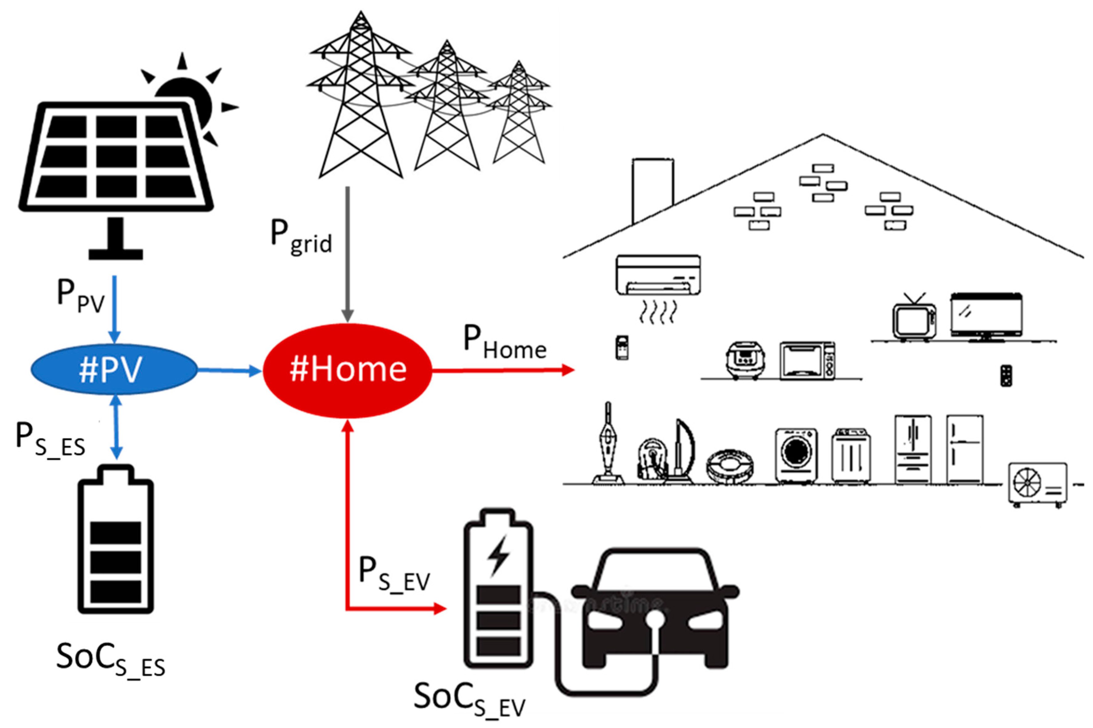
• This paper presents a formulation for the energy management of a detached residential house with CAEVs (G2V and V2G), PV generation and BESS units. Uncertainties regarding PV generation and CAEV mobility are incorporated into the optimization problem. The objective of the HEMS proposed is to manage the controllable energy resources: CAEV battery and BESS energy management to reduce the residential power grid demand from the grid and, consequently, the installation electricity bill.
• CAEV drivers’ range anxiety is incorporated as a reward term into the HEMS RL problem. This term penalizes the possibility of not having fully charged CAEV batteries at departure time. To the best of the authors’ knowledge, CAEV customers’ range anxiety is rarely incorporated into the HEMS RL problem.
• To optimize the CAEV charging/discharging improving the battery life, a punishment term regarding battery aging due to cycling operation is included in the RL formulation. This term penalizes repetitive charging/discharging operations during G2V and V2G processes, and it is considered a key aspect of HEMS.
• The RL rewards among energy consumption from the grid, range anxiety and battery aging are considered in the HEMS formulation based on a PPO algorithm that considers a tradeoff among the three individuals reward/punishment terms. To the best of the authors’ knowledge, range anxiety, combined with battery aging and G2V–V2G flexibility services, has scarcely been studied in HEMS research.
• A comparison with non-optimized and deterministic solutions was conducted to highlight the superiority of the proposed PPO-based HEMS system in terms of energy cost reduction. The results show the superiority of the PPO over the non-optimized and deterministic methods on the relative daily energy cost.

The rest of this paper is organized as follows: Section 2 presents the HEMS problem definition. Section 3 is devoted to Markov decision problem formulation. In Section 4, the PPO optimization is presented. Section 5 shows the results of the proposed HEMS via PPO implementation. The conclusions of the paper are summarized in Section 6.

2. Residential EV Management with PV Energy Sources and EV

2.1. Problem Definition

In this paper, an HEMS was developed to optimally integrate the energy management of CAEVs with V2G capabilities. The detached residential house installation includes photovoltaic generators (PV panels and a BESS unit) and a bidirectional wall box for the CAEV.

Figure 2 shows the energy scheme for the HEMS, with two main electrical nodes: the “HOME node” and the “PV node”. The HOME node represents the connection point of the detached residential house to the grid, where the power demand of the house (P_Home) could be supplied not only by the grid (P_grid) but also by the energy stored in the CAEV batteries (P_{S_EV}) and PV-BESS storage units ($P_{S\_ES})$. In the PV node, PV panels ($P_{PV}$) were installed to provide power to the house ($P_{PV-Home}$) and to the CAEV ($P_{S\_EV}$); moreover, the excess PV energy could be stored in the BESS unit ($P_{S\_ES}$).

In Figure 2, at the HOME and PV nodes, the energy balance set out in Equations (1) and (2) must be met:

$$P_{S\_EV}+P_{Home}=P_{grid}+P_{PV-Home}$$

(1)

$$P_{PV}=P_{S\_ES}+P_{PV-Home}$$

(2)

In Equation (2), at the PV node, the PV panels provide energy to the residential house ($P_{PV-Home}$) when there is sunlight ($P_{PV}$). The excess PV produced is stored in the BESS ($P_{S\_ES}$) and can be used to provide energy to the house for hours without PV production.

According to Figure 2, it was considered that the battery of the photovoltaic system can only be charged through the photovoltaic panel (PV node), reflected in (3), and so it is considered that the PV BESS unit cannot be charged through the grid or though the EV.

$$P_{PV-Home}\left(t\right)\ge 0$$

(3)

According to (1), the CAEV can be fed by the grid in the charging mode (G2V) or inject power into the grid (V2G) during discharging. The CAEV charging station is responsible for the bidirectional energy flow between the grid and the vehicle, which are limited by the charging station power limits ($P_{EV\_station,min}$, $P_{EV\_station,max}$) (4).

$$P_{EV\_station,min}\le P_{EV}\left(t\right)\le P_{EV\_station,max}$$

(4)

Traditional CAEV manufacturers recommend preserving the battery operation SoC between a minimum ${SoC}_{S\_EV,min}(10–20\%)$ and a maximum ${SoC}_{S\_EV,max}(80–100\%)$ (5) in order to avoid battery degradation due to thermal runaways and dissolution of active materials during discharging, and also to prevent overcharging and explosions during charging.

$${SoC}_{S\_EV,min}\le {SoC}_{S\_EV}\left(\mathit{t}\right)\le {SoC}_{S\_EV,max}$$

(5)

The BESS unit is charged via the PV’s surplus generation considering the BESS power socket’s limits ($P_{S\_ES,min}$, $P_{S\_ES,max}$) (6)

$$P_{S\_ES,min}\le P_{S\_ES}\left(\mathit{t}\right)\le P_{S\_ES,max}$$

(6)

Equation (7) represents the BESS state of charge constraints (${SoC}_{S\_ES,min}$,${SoC}_{S\_ES,max}$) associated with the PV generation unit. To protect the PV storage unit, the BESS state of charge (${SoC}_{S\_ES})$ must be kept over the ${SoC}_{S\_ES,min}$ and under the ${SoC}_{S\_ES,max}$ limits to avoid harmful and dangerous operation.

$${SoC}_{S\_ES,min}\le {SoC}_{S\_ES}\left(\mathit{t}\right)\le {SoC}_{S\_ES,max}$$

(7)

2.2. Home Energy Management

In this paper, three different objectives are considered in the RL process: the first is based on the minimization of the purchased electricity from the grid at the installation connection point ($C_{grid}$); the second objective penalizes EV departure with an empty battery or without a sufficient amount of stored energy for the daily trip, and is referred to as the battery fear cost or range anxiety cost ($C_{anx}$); and the third objective is based on battery degradation due to the cycling process ($C_{aging}$). The objective function is a balanced tradeoff among the three objectives (8).

$${C_{total}=C_{grid}+C_{anx}+C}_{aging}$$

(8)

It has to be noted that if the range anxiety ($C_{anx}$) is prioritized, the process of discharging (selling the stored energy to the grid) when electricity prices are high and charging (buying energy from the grid when electricity prices are low) could be limited. On the contrary, if the minimization of the purchased electricity from the grid is prioritized, the CAEV battery could not be fully charged at departure time. Similarly, if battery degradation cost is prioritized, then the battery cycling process is reduced, affecting both the total electricity cost and anxiety cost.

2.2.1. Energy Cost

The HEMS works for N_s time slots. The electric energy cost for a time slot, Δt, is a function of the power imported from the grid ($P_{grid}$) and the electricity cost (λ_eg) in each time slot (9):

$$C_{grid}={\sum }_{\begin{array}{c}k=0\\ t=t_0+k∆t\end{array}}^{k=N_s}{P}_{grid}{\lambda }_{eg}\left(t\right)\mathsf{\Delta }t$$

(9)

where t₀ is considered the beginning of the day.

2.2.2. Battery Fear Cost

The battery fear (anxiety) cost is an attempt to penalize the difference between the battery SoC at the departure time (${SoC}_{S\_EV(t=t_{dep})}$) and the driver’s required battery SoC (${SOC}_{EV,max}$) at the beginning of the day (10).

$$C_{anx}=K_1\left(1-\frac{{SoC}_{S\_EV\left(t=t_{dep}\right)}}{{SoC}_{S\_EV,max}}\right)$$

(10)

2.2.3. Battery Degradation Cost

The battery degradation cost is an attempt to penalize the batteries’ repetitive charge/discharge cycles during consecutive periods of time, which increase battery aging. This cost applies both to the battery of the CAEV, $C_{env-S\_EV}$, and to the battery of the PV installation, $C_{env-S\_ES}$ (11).

$$C_{aging}={\sum }_{\begin{array}{c}k=0\\ t=t_0+k∆t\end{array}}^{k=N_s}\left(C_{env-S\_EV}\left|P_{S\_EV}\left(t\right)\right|+C_{env-S\_ES}\left|P_{S\_ES}\left(t\right)\right|\right)\mathsf{\Delta }t$$

(11)

3. Markov Decision Process Formulation

In this paper, the HEMS problem is formulated as a Markov decision process (MDP) for sequential decision problems where the effects of the selected actions are unknown. A MDP is characterized by a tuple of four elements, {$S,a,T,R$}, where $S$ is the finite set of state space, $a$ is the set of actions, $T$ is the transition function and $R$ is the reward. The process evolution starts with an action ($a_k$), based on the observed state ($s_k$), which moves to the next state ($s_{k+1}$) through the transition function obtaining the corresponding reward ($r_k$).

3.1. State Space

The state space comprises the observations $s_kϵS$ that define the current situation in the environment at instant time $t$. For the HEMS defined in this paper (Figure 2), the environment is composed of: a detached house, a PV generation unit installed in the rooftop of the house, a BESS unit that stores the surplus energy provided by the PV installation, and a CAEV with a battery able to provide G2V and V2G services. The environment is defined by the power balanced equation at the HOME and PV nodes (1)–(3). According to this, the HEMS state space $S$ is a real-valued vector formed from:

-

the SoCs of the EVs batteries and PV units storage units (SoC_{S_EV,k}, SoC_{S_ES,k});

-

the EV departure time and plugged availability (t_s,dep, Plugged_EV,k);

-

the energy demand of the detached house (P_home);

-

PV production and information regarding the time slot (P_PV, t_s);

-

the electricity price (λ_eg).

Table 2. States/observations.

States	Description	Range
ts	Daily time	[t0: t0 + Ns Δt]
SoCS_ES,k	BESS storage SoC	[SoCS_ES,min: SoCS_ES,max]
SoCS_EV,k	CAEV Battery SoC	[SoCS_EV,min: SoCS_EV,max]
PluggedEV,k	Flag EV plugged into the grid	[0 (disconnected): 1 (connected)]
ts,dep	Time slot departure	[t0: t0 + Ns Δt]
λeg	Energy price	EUR/kWh
Phome	Residential demand	kWh
PPV	PV generation	kWh

shows the state space for the HEMS defined in this paper, with the states, definitions and range.

3.2. Action Space

The space action $A$ represents all valid actions for a given environment in each time slot, $a_kϵA$. In this paper, the HEMS action space $A$ is composed of two actions:

• The action regarding the charging/discharging orders of the PV-associated storage unit (BESS) ($a_{S\_ES}$),
• The action regarding the charging/discharging orders of the CAEV battery ($a_{S\_EV}$).
• The charge/discharge action $a_{S\_ES}$ determines, for each time slot, the amount of bidirectional energy flow between the PV generation and its associated storage unit (BESS). For the case of CAEV, the charging/discharge action $a_{S\_EV}$ for EV batteries is limited by the maximum charging/discharging power that could flow through the EV battery socket. When the action’s value is zero, there is no power flow between the charging socket and the battery. Both actions ($a_{S\_ES},a_{S\_EV}$) are continuous and are measured in kW.

3.3. Transition Function

In an MDP, the movement from state $s_k$ to the next state $s_{k+1}$ is driven by an action, $a_k$. The transition function provides information about the probability of reaching state $s_{k+1}$ from state $s_k$—that is, the probability of apply a trajectory $\tau$. For the HEMS proposed in this paper, the transition function drives the charging/discharging process of the available storage units:

• The transition function associated with the energy management of CAEVs: the charging/discharging of EV batteries.
• The transition function associated with the energy management of PV storage units: the charging/discharging of BESS batteries.

3.3.1. The Transition Function of CAEV Energy Management

The transition function of a CAEV’s battery is responsible for the charging/discharging of the EV battery through the action $a_{S\_EV}$. It must be highlighted that the charging/discharging of the EV will only be possible when the CAEV is connected to the grid (flag “Plugged_EV,k” = 1).

Equation (12) represents the transition function of EV energy management for the HEMS. The objective of (12) is to determine the new SoC of EV battery at instant $k+1$ after the application of action $a_{S\_EV,k}$ at instant $k$. In (12) for a given instant in time $k$, the value of the EV battery’s SoC in the following time instant, $k+1$ (${SoC}_{S\_EV,k+1}$), is given by the EV battery’s SoC at instant $k$ (${SoC}_{S\_EV,k}$) and the charge/discharge action ($a_{S\_EV}$) for the time slot Δt.

$${SoC}_{S\_EV,k+1}={SoC}_{S\_EV,k}+a_{S\_EV}\mathsf{\Delta }t$$

(12)

The EV battery’s SoC for a given instant k is limited by the maximum and minimum SoC constraints (5)—that is, it must be between ${SoC}_{S\_EV,min}($%) and ${SoC}_{S\_EV,min}($%) in order not to damage the battery.

CAEVs have two operation modes: G2V for the battery charging and V2G for the discharging. Charging or discharging action at instant $k$ is selected according to the current state or observation of the environment, the learning process regarding previous states, the selected action and the rewards.

• CAEV charging:

If the vehicle is connected to the electricity grid, it can be charged until the CAEV state of charge, ${SoC}_{S\_EV,k+1}$, reaches the maximum permitted value ${SoC}_{S\_EV,max}$ (13):

$${SoC}_{S\_EV,k+1}\le {SoC}_{S\_EV,max}$$

(13)

The charging power process in the V2G mode is shown in (14):

$$P_{S\_EV,k}=\min \left(P_{S\_EV,max},\frac{{SoC}_{S\_EV,max}-{SoC}_{S\_EV,k+1}}{∆t}\right)$$

(14)

Once the CAEV charging action ($P_{S\_EV,k}$) is obtained from (14), the EV battery SoC (${SoC}_{S\_EV,k+1})$ is updated in each iteration $k$ by (15):

$${SoC}_{S\_EV,k+1}={SoC}_{S\_EV,k}+\frac{\left(P_{S\_EV,k}∆t\right)}{{S\_EV\_bat}_{capacity}}$$

(15)

where ${SoC}_{S\_EV,k}$ is the EV battery SoC in the previous state $k$, ${S\_EV\_bat}_{capacity}$ is the CAEV battery capacity, and the term $\frac{\left(P_{S\_EV,k}∆t\right)}{{S\_EV\_bat}_{capacity}}$ represents the increase in the EV battery SoC as a consequence of action $a_{S\_EV,k}$ at instant $k$.

• CAEV discharging:

In the discharging mode (V2G), the CAEV SoC decreases until it reaches a minimum admissible value, ${SoC}_{S\_EV,min}$, through applying (16):

$${SoC}_{S\_EV,min}\le {SoC}_{S\_EV,k+1}$$

(16)

$$P_{S\_EV,k}=\max \left(P_{S\_EV,min},\frac{-{SoC}_{S\_EV,k+1}-{SoC}_{S\_EV,min}}{∆t}\right)$$

(17)

During discharging, the EV state of charge ${SoC}_{S\_EV,k+1}$ is updated in each iteration with (15).

3.3.2. PV Storage Energy Management Transition function

The transition function for the BESS storage unit (associated with the PV installation) during the charging/discharging process is driven by (18) and (19), respectively:

$$P_{S\_ES,k}=\min \left(P_{S\_ES,max},P_{S\_ES},\frac{{SoC}_{S\_ES,max}-{SoC}_{S\_ES,k+1}}{∆t}\right)$$

(18)

$$P_{S\_ES,k}=\max \left(P_{S\_ES,min},\frac{-{SoC}_{S\_ES,k+1}-{SoC}_{S\_ES,min}}{∆t}\right)$$

(19)

In order to determine the BESS transition charging function (18), the following items must be considered: the maximum energy that could flow between the PV generation unit and its associated BESS ($P_{S\_ES,max}$), the PV production at instant $k$ ($P_{S\_ES}$), and the increment in the BESS SoC as a consequence of action $a_{S_{ES}}$. The final transition charging action is the minimum value of these three items.

For the BESS transition discharging function (19), only two items are considered: the minimum energy flow between the PV generation unit and its associated BESS ($P_{S\_ES,min}$), and the decrement in the BESS SoC as a consequence of action $a_{S_{ES}}\mathrm{a}\mathrm{t}\mathrm{i}\mathrm{n}\mathrm{s}\mathrm{t}\mathrm{a}\mathrm{n}\mathrm{t}k$. The final transition discharging action is the maximum between these two items.

In each iteration step, $∆t$, the PV storage SoC, ${SoC}_{S\_ES,k+1}$, is updated with (20):

$${SoC}_{S\_ES,k+1}={SoC}_{S\_ES,k}+\frac{\left(P_{S\_ES,k}∆t\right)}{{S\_ES\_bat}_{capacity}}$$

(20)

where ${SoC}_{S\_ES,k}$ is the BESS SoC at instant $k$, ${S\_ES\_bat}_{capacity}$ is the battery capacity of the PV storage unit, and the term $\frac{\left(P_{S\_ES,k}∆t\right)}{{S\_ES\_bat}_{capacity}}$ represents the BESS SoC modification as a consequence of action $a_{\mathrm{S}\_\mathrm{E}\mathrm{S},k}$ at instant $k$.

3.4. Reward

In an MDP, the agent executes an action ($a_{S\_EV}$) that transitions to the next state ($s_{k+1}$) and calculates the reward $r_k$ of state $s_k$. In this HEMS problem formulation, the reward $r_k$ is determined by the following terms:

• The revenues/expenses due to the consumption or injection of electrical energy at the connection point of the residential house (21) which depend on the energy purchased from the grid ($P_{grid}$) and the price of the energy (${\lambda }_{eg,k}$) at instant time $k$.

$$r_{k,ele}=P_{grid}{\lambda }_{eg,k},\mathsf{\Delta }t$$

(21)

• The expenses incurred due to batteries’ degradation (CAEV, PV storage), which are shown in (22), depend on the amount of charged or discharged power on these units ($P_{S\_EV,k}$, $P_{S\_ES,k}$) multiplied by the weight factors of EV battery degradation ($C_{env-S\_EV})$ and BESS storage degradation and ($C_{env-S\_ES}$).

$$r_{k,aging}=(C_{env-S\_EV}\left|P_{S\_EV,k}\right|+C_{env-S\_ES}\left|P_{S\_ES,k}\right|)\mathsf{\Delta }t$$

(22)

• The range anxiety expense is associated with the uncompleted SoC of the EV at the departure instant. At this instant, ($t=t_{dep}$), the range anxiety reward calculates the difference between the maximum SoC of the electric vehicle battery and the current SoC at departure time, as shown in (23).

$$r_{k,fear}=\left\{\begin{array}{cc}{K}_1\left(1-\frac{{SoC}_{S\_EV,k}}{{SoC}_{S\_EV,max}}\right)& ift=t_{dep}\\ o& else\end{array}\right.$$

(23)

Finally, the total reward for a slot time, $k$, is composed of the combined rewards of each individual component (24).

$$r_k=r_{k,ele}+r_{k,fear}+r_{k,aging}$$

(24)

4. Proximal Policy Optimization

Proximal policy optimization (PPO) belongs to the family of value-based and policy gradient algorithms. PPO is a model-free RL algorithm focused on policy gradient optimization where the policy is updated in each iteration using the clipping and subrogate function. One of the advantages of the PPO is that its formulation helps to maximize exploration in the learning process without increasing the computational complexity of the algorithm. The policy is updated by the policy gradient theorem to increase the expected reward. In PPO, the agent is composed of critic and actor modules (actor–critic). The actor’s objective is to determine the optimal policy, considering the environment, to maximize the reward. Therefore, the actor module is responsible for generating the action of the system, $a_k$, represented by the policy ${\pi }_{\theta }$, and parameterized by $\theta$. The critic module estimates the value function of the state of the system ($V_{\mu }\left(s_k\right)$) (Figure 3)—that is, the critic module evaluates the agent action by means of the value function $V_{\mu }$ parametrized by $\mu$. To estimate the expected cumulative reward, the critic module uses the Q-value function. The critic’s output value is used by the actor to adjust policy decisions, leading to a better return.

As can be seen in Figure 3, the input of both modules is the state space at time k. Moreover, the critic module has the reward as a second input. The output values of the critic module are the input of the actor module to adjust the policy. The actor module’s output is the action over the time, $k$, according to policy ${\pi }_{\theta }$.

PPO uses an extended function to iteratively enhance the target function ($L^{clip}$) by clipping the objective function to keep the new policy close to the old one. These updates are limited in order to prevent large policy variations and to improve training stability. Equation (25) shows PPO-clip update policies.

$${\theta }_{k+1}=\arg \underset{\theta }{\max }{\mathbb{E}}_{s,a~{\pi }_{{\theta }_k}}\left[L^{clip}\left(s,a,{\theta }_k,\theta \right)\right]$$

(25)

where $L^{clip}\left(s,a,{\theta }_k,\theta \right)$ (26) is the surrogate advantage function [32]. The surrogate advantage function measures the performance of the new policy ${\pi }_{\theta }$ according to the old policy ${\pi }_{{\theta }_k}$.

$$L^{clip}\left(s,a,{\theta }_k,\theta \right)=\left(\min (\frac{{\pi }_{{\theta }_k}\left(\left.s\right|a\right)}{{\pi }_{\theta }\left(\left.s\right|a\right)}{\widehat{A}}_{\theta }\left(s,a\right),clip\left(\frac{{\pi }_{{\theta }_k}\left(\left.s\right|a\right)}{{\pi }_{\theta }\left(\left.s\right|a\right)},1-ϵ,1+ϵ\right){\widehat{A}}_{\theta }\left(s,a\right)\right)$$

(26)

where $ϵ$ is a hyperparameter used for reducing the policy variations. ${\widehat{A}}_{\theta }\left(s,a\right)$ (27) is an advantage function used to measure the difference between the expected reward provided by the Q-function and the average reward provided by the value function $V\left(s\right)$, of a policy ${\pi }_{\theta }\left(\left.s\right|a\right)$. The objective of the advantage function is to give a relative measure (average) of the goodness of an action, instead of an absolute value.

$${\widehat{A}}_{\theta }\left(s,a\right)=Q\left(s,a\right)-V\left(s\right)$$

(27)

A simplified version of (26) can be find in (28):

$$L^{clip}\left(s,a,{\theta }_k,\theta \right)=\left(\min (\frac{{\pi }_{{\theta }_k}\left(\left.s\right|a\right)}{{\pi }_{\theta }\left(\left.s\right|a\right)}{\widehat{A}}_{\theta }\left(s,a\right),g\left(ϵ,{\widehat{A}}_{\theta }\left(s,a\right)\right)\right)$$

(28)

where $g\left(ϵ,{\widehat{A}}_{\theta }\left(s,a\right)\right)$ is defined in (29):

$$g\left(ϵ,{\widehat{A}}_{\theta }\left(s,a\right)\right)=\left\{\begin{array}{cc}(1+ϵ){\widehat{A}}_{\theta }& {\widehat{A}}_{\theta }\ge 0\\ (1-ϵ){\widehat{A}}_{\theta }& {\widehat{A}}_{\theta }<0\end{array}\right.$$

(29)

In (29), a positive advantage function relies on a better outcome. On the contrary, a negative advantage function value feedback indicates that the actor needs to explore new actions to improve the policy performance.

The implementation of the algorithm is shown in Algorithm 1

Algorithm 1. PPO, Actor-Critic pseudocode
Require: Initialize actor-critic network with parameter θ, μ, clipping threshold ∊, and a storage buffer D for trajectory memory
1	for each step of an episode do
2	for  k = 1…T do
3	get initial state s
4	select the action $a_k$ from actor network, ${\pi }_{\theta }\left(s\right)$
5	run the action $a_k$ through the environment obtain the reward $r_k$ from the critic network, and next state s’
6	Update the actor-critic network parameters
7	store the tuple {S, a, T, R} in the replay buffer D
8	$s\leftarrow s^{\prime }$
9	end for
10	end for

5. Practical Implementation

In this section, a HEMS composed of a single CAEV and a solar installation with a storage unit is solved with a PPO algorithm. The HEMS’s objectives are threefold: (i) to reduce the house’s power demand for electricity from the grid; (ii) to improve battery life (CAES, BESS); and (iii) to minimize CAEV drivers’ anxiety.

5.1. Dataset Description

In this paper, we adopted real data for the home electricity demand of a typical Spanish detached house. The house’s daily energy demand was fixed at 11.4 kWh. The dataset used for training and testing comprised a range of data from January 2021 to June 2021, with a 10 min time resolution [33], which were used directly in the process without performing any preprocessing of data.

The detached house had a PV rooftop installation of 3 kW with a battery storage unit of 10 kWh. The storage unit had a bidirectional socket of 3 kW for the charging/discharging process. The PV data was obtained from [33] with a 10 min resolution.

Moreover, a CAEV (24 kWh) was available in the installation and could charge/discharge its battery with a maximum charging/discharging power of 7.5 kW. The CAEV was able to provide energy to the grid in the V2G mode. The CAEV departure time, the CAEV arrival hours and the SoC at arrival (in p.u. values) each followed a normal distribution: N(08, 1.0), N(19, 1.5) and N(0.5, 0.2), respectively (Figure 4).

Storage units (EV battery and BESS) where considered to have SoC operation limits of ${SoC}_{min}=20\%$ and ${SoC}_{max}=100\%$, which are the typical limits recommended by batteries manufacturers.

Finally, the day-ahead electricity prices of the Iberian market were obtained from [33].

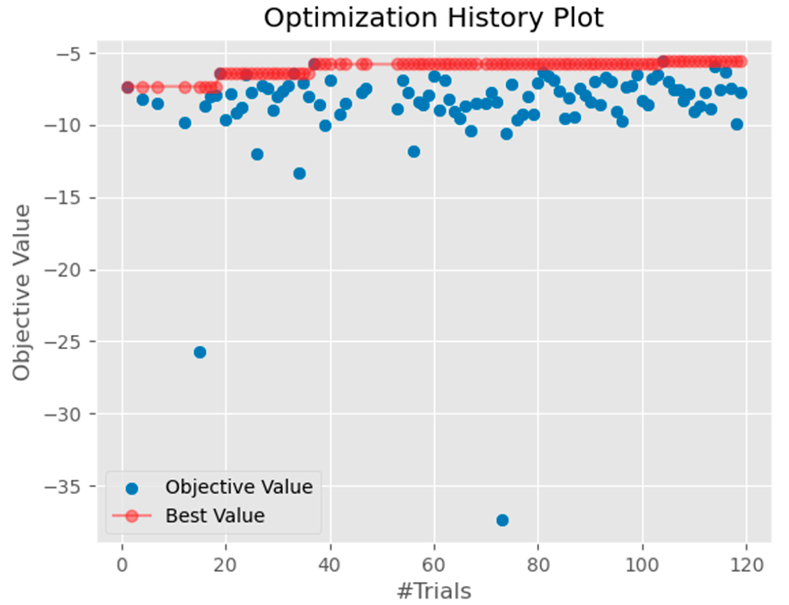
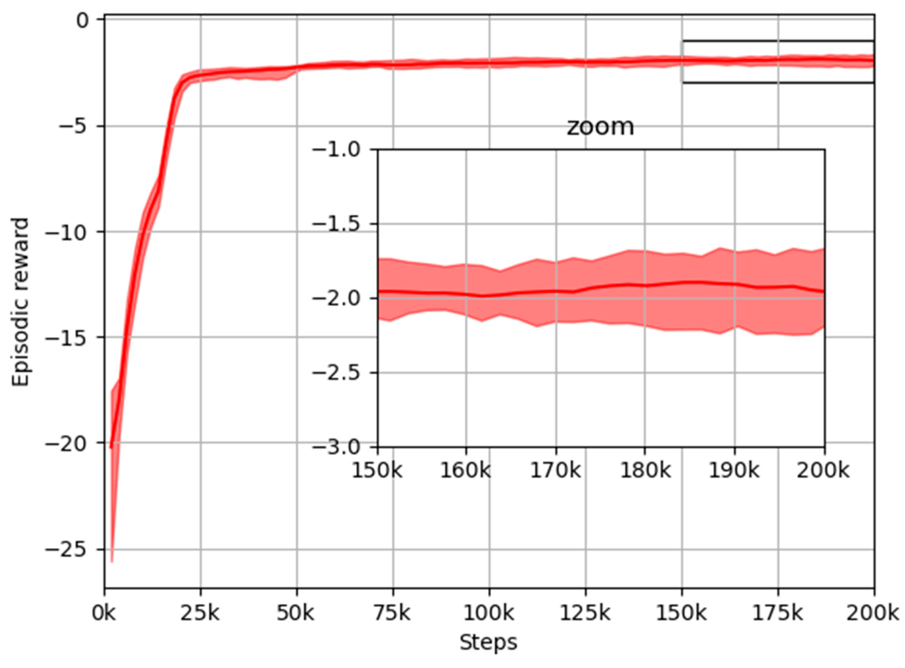
5.2. PPO Training

The complete dataset was divided into two groups: two-thirds of the data were used for training (4 months) and one-third of the data were used for validation (2 months). The operation horizon was 24 h. The time slot considered for PPO training and validation was 10 min, so that T = 144.

An Optuna framework [34] was used to select the optimal hyperparameters for the implementation of the HEMS’s PPO considering different algorithms such as evolutionary methods and Bayesian methods, with the objective of reaching a balance between sampling and pruning. Optuna is able to obtain the optimal solution iteratively by solving the PPO objective function. In this paper, the Optuna framework was used for obtaining the value of three hyperparameters of the PPO formulation: the learning rate hyperparameter, which can take values from 0.00001 to 0.0010; the number epoch hyperparameter, where Optuna varies its value from 10 to 200 in each iterative search; and the gamma hyperparameter, which ranges from 0.9990 to 0.9999.

Figure 5 shows the evolution of the Optuna hyperparameter selection.

In the HEMS proposed in this paper, actor and critic modules are implemented with deep neural networks (DNNs). The selection of the optimal number of deep layers is not a trivial task; if the number of deep layers is too high, there can be problems of overfitting. In this paper, both networks were formed by three layers because the number of deep layers is quite small, providing good accuracy and fast performance. Increasing the number of deep layers did not provide any improvement and, on the contrary, it increased the computational complexity slowing the convergence process. Similarly, a high number of neurons per layer increases the computational cost. In this work, 16 neurons per layer in both the actor and critic network [16] provided both good accuracy and low computational cost. In a deep learning model, several activation functions can be applied ($Relu$, $tanh$, $Sigmoid$). In general, the $Sigmoid$ function is used as an output activation function with binary classification problems. The $Relu$ function has the disadvantage of generating dead neurons which do not contribute to the decision-making process. In this work, the hyperbolic tangent ($tanh$) activation function was considered for both the actor and the critic network because the accuracy is high, and it provides zero-centered mapping positive and negatives values, which is very suitable for our implementation.

Finally, Stable-Baselines3 [35] was used to implement the PPO in Python. The optimal hyperparameters of the PPO formulation of the HEMS problem are as follows (objective e-value: 5.590105):

-

Learning rate: 0.000436

-

Gamma: 0.999155

-

N_step = 2048

-

Gae (γ): 0.95

-

Batch size = 64

-

Clip_range = 0.2

-

Number epoch: 37

-

Entropy coef = 0.0005

-

Number eval_episodes = 5

-

Total time steps = 200,000

Figure 6 shows the training process and the convergence performance of the proposed PPO algorithm. It is designed to be tested every 10 epochs and take the average cumulative cost of five repetitions. From Figure 6, it can be noted that the reward experiences a great increase in the training process until 25,000 steps. This is due to the lack of experience and limited iteration data. After this point, the training curve converges to a stable policy, so that the episodic reward is smoothened, and converges to the optimal reward as the number of steps increases up to a time step total over 200,000.

5.3. Energy Management with the PPO

Figure 7, Figure 8 and Figure 9 show the energy management of the PV storage and the EV batteries for four consecutive days for the sake of clarity.

(a)

Power consumption from the grid

In Figure 7, the net active power evolution imported from the grid (blue), the power demand of the residential house (yellow) and the power injection from the PV installation to the house (green) can be seen. The red curve shows the electricity cost. It can be observed in Figure 7 that, for most hours of the day, the house’s power demand is fed either by the power coming from the PV and BESS units,$P_{PV-Home}$ (green), or by the EVs; thus, the energy imported from the grid, $P_{grid}$(blue), is mainly required for EV charging at night (from 3:00 to 6:00 h a.m.). It can also be noted that there is a negative power consumption from the grid in the period of 18:00–21:00 h, which corresponds to power injection into the grid by the CAEV (V2G capability).

(b)

BESS energy management

Figure 8 shows the energy management of the PV storage and its storage unit (BESS). It can be seen in Figure 8 that the energy that PV produced (yellow line) was stored in the storage units (blue lines) during most of the PV working hours. Additionally, the PPO algorithm optimized the energy management of the energy stored in the PV storage unit; when there was an excess of PV produced (sunlight) from 13:00 to 18:00 h, the PV storage unit was charged, $E_{ES}\left(red\right),$ in these situations. On the contrary, at night (from 20:00 to 23:00 h), the PV storage unit injected the stored energy (red) into the residential house.

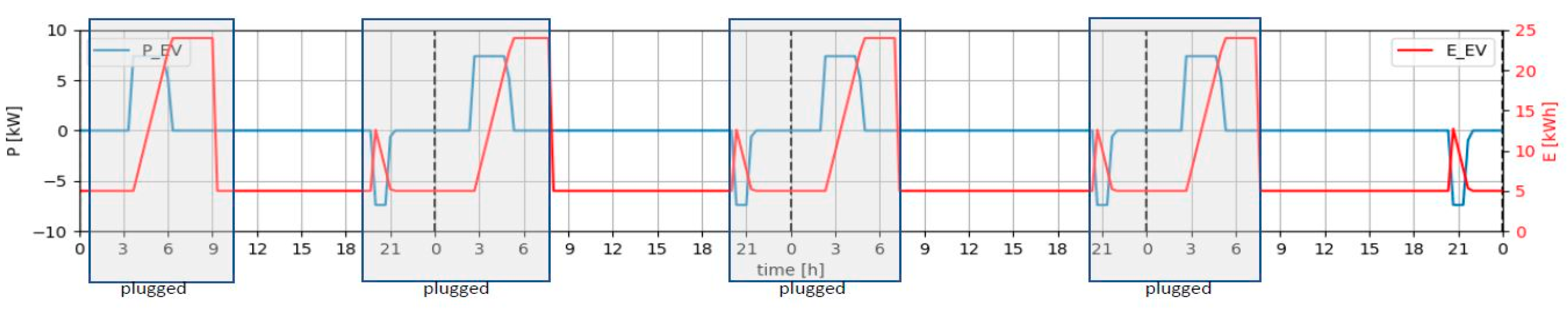
(c)

CAEV energy management

Figure 9 shows the EV energy management; the blue curve represents the active power consumed by the vehicle (positive) or injected (negative) during charging and discharging, respectively. The red lines represent the energy stored in the EV battery during charging and discharging, and the gray boxes denote the hours that the EV was plugged in. Furthermore, it can be noted that the PPO algorithm controlled the CAEV battery for providing energy to the grid (V2G) when electricity prices were high, and charging was delayed until the moments when the electricity costs were lower. In addition, there were moments when the power from the grid ($P_{grid}$) was negative (Figure 7), in which the EV was injecting power into the grid that was operating in the V2G mode.

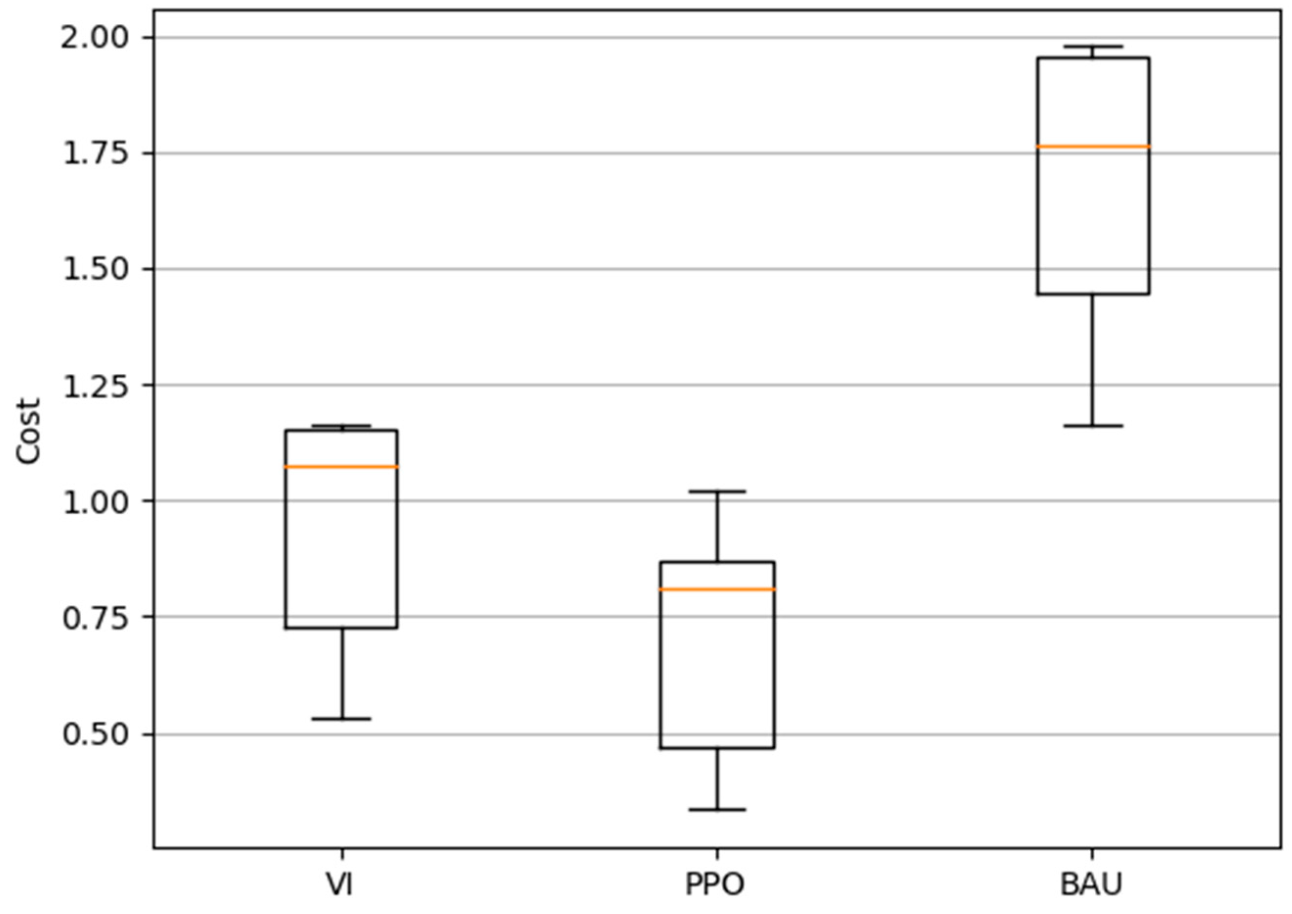
5.4. Total Cost Comparison

To validate the proposed PPO algorithm, the results obtained were compared to the business-as-usual (BAU) and value iteration (VI) schemes.

-

In the BAU scheme, any optimization is performed over the controllable loads. In this scheme, the CAEVs were connected to the grid and the charging process started without delay as soon as they arrived at the house. This scheme did not use information regarding energy prices, and only the G2V mode was allowed for the CAEVs.

-

The value iteration solution scheme (VI) is a deterministic method, with a low percentage of uncertainties in the information, and perfect knowledge of the model. This method lies in the beginning of RL algorithms. VI relies on the acquisition of the optimal policy for an MDP by calculating the value function ($V_{\pi }\left(s_k\right)$), defined as (30), where $\gamma$ represents the discount factor considering the uncertainty associated with future costs and ensures that the return ($r_k$) is a finite value.

$$V_{\pi }\left(s_k\right)=r_k+\gamma V_{\pi }\left(s_{k+1}\right)$$

(30)

The goal of VI is to find the policy π that maximizes the return over time (a day), learning by interacting with the environment. The VI algorithm learns from past experiences through the bootstrapping technique, and the value function is obtained from previous estimates. In the comparison between the HEMS proposed in this paper and the VI scheme, the value iteration estimated the goodness of being in a certain state, and the Bellman optimality equation in (30) used a greedy policy that selected the best action using the $V_{\pi }\left(s_{k+1}\right)$ function.

The energy management cost comparison between BAU, VI and the PPO is shown in Figure 10. It can be noted that in the business-as-usual scheme, the charging process is not controlled and V2G is not available; consequently, this solution is the most expensive, with a relative daily energy cost of 1.75 EUR/kWh.

VI is a deterministic method, based on dynamic programming, which is not suitable for dealing with continuous stochastic problems, consequently limiting its application to solve real problems. The final energy management relative daily energy cost for the VI solution was 1.1 EUR/kWh. The value iteration solution represents a cost improvement of 37% compared to the BAU scheme.

The proposed PPO scheme deals with uncertainties associated with stochastic PV generation and uncertain CAEV mobility (random arrival and departure time and unknown SoC at connection time), as well as high variability in electricity market prices. PPO performance was the best of the three schemes analyzed, with a total relative daily energy cost of 0.8 EUR/kWh. The relative cost improvement of the PPO over BAU and VI schemes is 54% and 27%, respectively. Moreover, the PPO deals with continuous action-space and continuous state space, while the VI solutions require discrete values, which limits its performance in complex problems.

6. Conclusions

In this paper, we proposed a home energy management of a smart home where the load demand is non-controllable. The residential installation is composed of a CAEV and PV panels with storage units. The algorithm concurrently manages the charging and discharging processes of two different storage units: one associated with PV rooftop generation and the other with the EV battery, which has V2G–G2V capabilities. The objectives of the HEMS were threefold: to reduce the home’s electricity power demand, to improve battery life (CAES, BESS) and to minimize CAEV drivers’ anxiety. Reinforcement learning techniques arose as the best solution to meet the HEMS objectives dealing with an environment characterized by high uncertainty due to stochastic PV generation, random EV mobility and high variability in market electricity prices. We introduced a PPO algorithm with an actor–critic framework to perform the optimal scheduling of daily charging/discharging for PV-BESS and CAEV storage units. Different rewards were considered for the definition of the MDP: expenses due to the consumption of electricity from the grid, expenses due to uncompleted CAEV SoC at departure time, and expenses due to the battery degradation cost.

To test the proposed HEMS based on a PPO actor–critic framework, the CAEV mobility pattern was simulated considering both random arrival and departure hours and random SoC at the connection hour. Moreover, our case study was conducted based on a real Spanish dataset of residential consumption, photovoltaic generation, and electricity prices.

The results show that the PPO was capable of solving optimal charging/discharging schemes for BESS storage units and CAEV batteries, showing its superiority compared to non-optimized methods (BAU: business-as-usual) and deterministic methods (VI: value iteration solutions). The PPO’s optimal charging/discharging schedule reduced the relative daily energy cost by 54% and 27% compared with BAU and VI, respectively.

It has to be noted that the proposed RL formulation focuses on the local energy management of a residential installation to optimize the energy consumption of a smart home, and so it does not need any knowledge about other customers connected to the power grid or other information regarding the distribution power grid. It was demonstrated that the developed PPO algorithm is suitable for real-time operations due to its fast execution and good convergence to the optimal solution. The proposed PPO is scalable to large residential installations with aggregated PV generation, several BESS units, and different numbers of electric vehicles. Moreover, the proposed RL approach can be modified to include in its formulation the energy management of controllable loads of a smart home.

References

- IEA. Transport, IEA, Paris. 2022. Available online: https://www.iea.org/reports/transport (accessed on 30 April 2023).
- Esmaili, M.; Shafiee, H.; Aghaei, J. Range anxiety of electric vehicles in energy management of microgrids with controllable loads. J. Energy Storage 2018, 20, 57–66. [Google Scholar] [CrossRef]
- Communication from the Commission to the European Parliament, the European Council, the Council, the European Economic and Social Committee and the Committee of the Regions. The European Green Deal. COM/2019/640 Final. Available online: http://eur-lex.europa.eu/LexUriServ/LexUriServ.do?uri=CELEX:52012DC0673:EN:NOT (accessed on 1 June 2023).
- Kempton, W.; Tomic, J. Vehicle-to-grid power fundamentals: Calculating capacity and net revenue. J. Power Sources 2005, 144, 268–279. [Google Scholar] [CrossRef]
- Alonso, M.; Amaris, H.; Martin, D.; De La Escalera, A. Energy management of autonomous electric vehicles by reinforcement learning techniques. In Proceedings of the Second International Conference on Sustainable Mobility Applications, Renewables and Technology (SMART), Cassino, Italy, 12 December 2022. [Google Scholar]
- V2G Hub Insights. Available online: https://www.v2g-hub.com/insights (accessed on 4 November 2022).
- Jian, L.; Zheng, Y.; Xiao, X.; Chan, C.C. Optimal scheduling for vehicle to-grid operation with stochastic connection of plug-in electric vehicles to smart grid. Appl. Energy 2015, 146, 150–161. [Google Scholar] [CrossRef]
- Lund, H.; Kempton, W. Integration of renewable energy into the transport and electricity sectors through V2G. Energy Policy 2008, 36, 3578–3587. [Google Scholar] [CrossRef]
- Al-Awami, A.T.; Sortomme, E. Coordinating vehicle-to-grid services with energy trading. IEEE Trans. Smart Grid 2012, 3, 453–462. [Google Scholar] [CrossRef]
- Shariff, S.M.; Iqbal, D.; Alam, M.S.; Ahmad, F. A state of the art review of electric vehicle to grid (V2G) technology. IOP Conf. Ser. Mater. Sci. Eng. 2019, 561, 012103. [Google Scholar] [CrossRef]
- Barbato, A.; Capone, A. Optimization Models and Methods for Demand-Side Management of Residential Users: A Survey. Energies 2014, 7, 5787–5824. [Google Scholar] [CrossRef] [Green Version]
- Carli, R.; Dotoli, M. Energy scheduling of a smart home under nonlinear pricing. In Proceedings of the 53rd IEEE Conference on Decision and Control, Los Angeles, CA, USA, 15–17 December 2014; pp. 5648–5653. [Google Scholar]
- Falvo, M.C.; Graditi, G.; Siano, P. Electric Vehicles integration in demand response programs. In Proceedings of the International Symposium on Power Electronics, Electrical Drives, Automation and Motion, Ischia, Italy, 18–20 June 2014; pp. 548–553. [Google Scholar]
- Scott, C.; Ahsan, M.; Albarbar, A. Machine learning based vehicle to grid strategy for improving the energy performance of public buildings. Sustainability 2021, 13, 4003. [Google Scholar] [CrossRef]
- Kern, T.; Dossow, P.; von Roon, S. Integrating bidirectionally chargeable electric vehicles into the electricity markets. Energies 2020, 13, 5812. [Google Scholar] [CrossRef]
- Sovacool, B.K.; Noel, L.; Axsen, J.; Kempton, W. The neglected social dimensions to a vehicle-to-grid (V2G) transition: A critical and systematic review. Environ. Res. Lett. 2018, 13, 013001. [Google Scholar] [CrossRef]
- Yao, L.; Lim, W.H.; Tsai, T.S. A real-time charging scheme for demand response in electric vehicle parking station. IEEE Trans. Smart Grid 2017, 8, 52–62. [Google Scholar] [CrossRef]
- Chen, H.; Hu, Z.; Zhang, H.; Luo, H. Coordinated charging and discharging strategies for plug-in electric bus fast charging station with energy storage system. IET Gener. Transm. Distrib. 2018, 12, 2019–2028. [Google Scholar] [CrossRef] [Green Version]
- Vagropoulos, S.I.; Bakirtzis, A.G. Optimal bidding strategy for electric vehicle aggregators in electricity markets. IEEE Trans. Power Syst. 2013, 28, 4031–4041. [Google Scholar] [CrossRef]
- Amin, A.; Tareen, W.U.K.; Usman, M.; Ali, H.; Bari, I.; Horan, B.; Mekhilef, S.; Asif, M.; Ahmed, S.; Mahmood, A. A review of optimal charging strategy for electric vehicles under dynamic pricing schemes in the distribution charging network. Sustainability 2020, 12, 10160. [Google Scholar] [CrossRef]
- Xu, Y.; Pan, F.; Tong, L. Dynamic scheduling for charging electric vehicles: A priority rule. IEEE Trans. Autom. Control 2016, 61, 4094–4099. [Google Scholar] [CrossRef]
- Chen, Q.; Folly, K.A. Application of Artificial Intelligence for EV Charging and Discharging Scheduling and Dynamic Pricing: A Review. Energies 2023, 16, 146. [Google Scholar] [CrossRef]
- Al-Ogaili, A.S.; Hashim, T.J.T.; Rahmat, N.A.; Ramasamy, A.K.; Marsadek, M.B.; Faisal, M.; Hannan, M.A. Review on scheduling, clustering, and forecasting strategies for controlling electric vehicle charging: Challenges and recommendations. IEEE Access 2019, 7, 128353–128371. [Google Scholar] [CrossRef]
- Lee, S.; Choi, D.H. Dynamic pricing and energy management for profit maximization in multiple smart electric vehicles charging stations: A privacy-preserving deep reinforcement learning approach. Appl. Energy 2021, 304, 117754. [Google Scholar] [CrossRef]
- Cedillo, M.H.; Sun, H.; Jiang, J.; Cao, Y. Dynamic pricing and control for EV charging stations with solar generation. Appl. Energy 2022, 326, 119920. [Google Scholar] [CrossRef]
- Moghaddam, V.; Yazdani, A.; Wang, H.; Parlevliet, D.; Shahnia, F. An online reinforcement learning approach for dynamic pricing of electric vehicle charging stations. IEEE Access 2020, 8, 130305–130313. [Google Scholar] [CrossRef]
- Sun, D.; Ou, Q.; Yao, X.; Gao, S.; Wang, Z.; Ma, W.; Li, W. Integrated human-machine intelligence for EV charging prediction in 5G smart grid. EURASIP J. Wirel. Commun. Netw. 2020, 2020, 139. [Google Scholar] [CrossRef]
- Boulakhbar, M.; Farag, M.; Benabdelaziz, K.; Kousksou, T.; Zazi, M. A deep learning approach for prediction of electrical vehicle charging stations power demand in regulated electricity markets: The case of Morocco. Clean. Energy Syst. 2022, 3, 100039. [Google Scholar] [CrossRef]
- Kaewdornhan, N.; Srithapon, C.; Liemthong, R.; Chatthaworn, R. Real-Time Multi-Home Energy Management with EV Charging Scheduling Using Multi-Agent Deep Reinforcement Learning Optimization. Energies 2023, 16, 2357. [Google Scholar] [CrossRef]
- Jin, J.; Xu, Y. Optimal Policy Characterization Enhanced Actor-Critic Approach for Electric Vehicle Charging Scheduling in a Power Distribution Network. IEEE Trans. Smart Grid 2021, 12, 1416–1428. [Google Scholar] [CrossRef]
- Zhang, C.; Li, T.; Cui, W.; Cui, N. Proximal Policy Optimization Based Intelligent Energy Management for Plug-In Hybrid Electric Bus Considering Battery Thermal Characteristic. World Electr. Veh. J. 2023, 14, 47. [Google Scholar] [CrossRef]
- Schulman, J.W.; Dhariwal, F.; Radford, P.; Oleg, A.; Oleg, K. Proximal Policy Optimization Algorithm. arXiv 2017, arXiv:1707.06347. [Google Scholar]
- Red Eléctrica Española. Sistema de Información del Operador del Sistema Eléctrico en España. Available online: https://esios.ree.es/en (accessed on 20 October 2022).
- Akiba, T.; Sano, S.; Yanase, T.; Ohta, T.; Koyama, M. Optuna: A next generation hyperparameter optimization framework. In Proceedings of the 25th ACM SIGKDD International Conference of the Knowledge Discovery & Data Mining, Anchorage, AK, USA, 4–8 August 2019; pp. 2623–2631. [Google Scholar]
- Raffin, A.; Hill, A.; Gleave, A.; Kanervisto, A.; Ernestus, M.; Dormann, N. Stable-Baselines3: Reliable Reinforcement Learning Implementations. J. Mach. Learn. Res. 2021, 22, 1–8. [Google Scholar]