Abstract
Combined heat and power generation is the simultaneous conversion of primary energy (in the form of fuel) in a technical system into useful thermal and mechanical energy (as the basis for the generation of electricity). This method of energy conversion offers a high degree of efficiency (i.e., very efficient conversion of fuel to useful energy). In the context of energy system transformation, combined heat and power (CHP) is a fundamental pillar and link between the volatile electricity market and the heat market, which enables better planning. This article presents an advanced model for the production of fuel mixtures based on landfill biogas in the context of energy use in CHP units. The search for optimal technological solutions in energy management requires specialized domain-specific knowledge which, using advanced algorithmic models, has the potential to become an essential element in real-time intelligent ICT systems. Numerical modeling makes it possible to build systems based on the knowledge of complex systems, processes, and equipment in a relatively short time. The focus was on analyzing the applicability of algorithmic models based on artificial intelligence implemented in the supervisory control systems (SCADA-type systems including Virtual SCADA) of technological processes in waste management systems. The novelty of the presented solution is the application of predictive diagnostic tools based on multithreaded polymorphic models, supporting making decisions that control complex technological processes and objects and solving the problem of optimal control for intelligent dynamic objects with a logical representation of knowledge about the process, the control object, and the control, for which the learning process consists of successive validation and updating of knowledge and using the results of this updating to determine control decisions.
1. Introduction
A modified simplex algorithm using greedy strategies was used to solve the scientific/technological problem. With regard to thermodynamic considerations, the use of local low-power combined heat and power (CHP) systems is a particularly favorable solution, leading to a reduction in the consumption of primary fuels compared to the separate and centralized production of energy carriers. High-efficiency cogeneration of a few to several hundred kWe can be carried out using an internal combustion engine fueled by landfill biogas. The implementation of CHP systems can significantly contribute to low-carbon heat and power generation [1,2].
The concept of producing fuel–air mixtures based on recovered landfill biogas for CHP units is essentially based on the following assumptions:
- Substances included in fuels have defined physicochemical and fueling properties;
- The combustion process involving landfill biogas in internal combustion engines that are part of the cogeneration unit is well-known. The course of the technological process of fuel component production is controlled by advanced SCADA-type supervisory control systems, providing process parameter monitoring, process visualization, and realizing complex control algorithms (including adaptive, predictive, and inferential control algorithms) through the use of freely programmable logic controllers (PLCs) [3,4,5]. The physical process of preparing fuel mixtures requires a thorough analysis of the physical and chemical properties of the ingredients of the fuel components as well as the technological considerations. The stringent requirements for the thermal decomposition of substances in spark-ignition reciprocating engines impose a number of requirements on fuels. Above all, they must have:
- The optimal calorific value (enthalpy of devaluation);
- Corresponding elemental composition, fuel properties (moisture content, content of flammable parts, content of non-flammable parts, content of volatile parts, content of aggressive components);
- Ignition temperature, combustion temperature [6,7,8].
The physical and energetic properties of the gas–air mixture supplied to the cylinders of an internal combustion engine determine the value of its performance (energy efficiency, torque, and power at a given speed value) as well as the extent of its harmful impact on the environment. Biogas-fueled internal combustion engines are units designed mainly by adapting an engine that typically operates on a liquid fuel (petrol, diesel) or a high-calorific gaseous fuel such as natural gas [9]. Stationary engines that drive electricity generators (typically with a power output in excess of 500 kW) are powered by a weak mixture of gas and air. Therefore, depending on the type of fuel used, the value of the chemical energy of the fuel–air mixture will depend to varying degrees on the value of the air excess ratio [10,11].
The performance of an internal combustion engine in a CHP unit, expressed in terms of torque and effective power at a specified engine speed, depends on the parameters of the fuel–air mixture. Spark-ignition engines use quantitative control of the gas–air mixture composition. This type of control involves throttling the amount of air supplied to the combustion engine depending on its load. Adequately to the amount of air, biogas is supplied to the cylinder in an amount that ensures that the engine operates with the required air excess ratio λ. The optimum fuel-to-air ratio when powering an internal combustion engine allows the expected effective power to be achieved with the lowest possible fuel consumption [12,13]. Control and monitoring of the lambda index value is crucial for the quality of the combustion of the fuel mixture in the context of gas and dust emissions into the air, affecting the environmental load of these pollutants.
Unlike others, the novelty of the presented solution is the application of predictive diagnostic tools based on multithreaded polymorphic models developed using MATLAB/Simulink tools. In particular, the automatic control system was based on a freely programmable PLC controller, in which a control algorithm was implemented that followed the reference trajectory of the methane and oxygen concentrations.
The algorithm controlling the operation of the solenoid valves implements/follows the reference trajectory of the demand/consumption of gaseous fuel by the internal combustion engine of the CHP unit. A change in the gas parameters in the degassing well causes an event of a change in the well’s operating state, and the detection system of these changes calls the method in response—a sequence of simplex, MC SVM, and greedy set cover (master algorithm) algorithms—and sets the value of the signal supplied by the PLC to the actuators (i.e., solenoid valves (open/close level)). As a result, the control algorithm (MPC—model predictive control) stabilizes the engine operation by reproducing the theoretical (as a reference) OTTO cycle, determining the optimal composition of the air–fuel mixture based on the determined shares of the streams of individual degassing wells, taking into account their operating characteristics and operating states (operating transmittances). The automatic control system is based on a freely programmable PLC controller, in which a control algorithm is implemented that follows the reference trajectory of the methane and oxygen concentrations.
The presented study is in line with contemporary strategic efforts to prevent climate change through the implementation of a closed-loop economy, with particular attention paid to the energy potential of biogas/biomethane in the context of its use in commercial and thermal power generation.
2. Materials and Methods
Research tools in the form of control using the MPC model were used in this work, allowing us to manage the technical infrastructure equipped with actuators, solenoid valves, analyzers, and to solve the research problem, which was the optimization of the gas–fuel mixture for the engine in a cogeneration unit.
2.1. The Research/Technological Problem
The research problem was solved by using the MPC model predictive control generating optimal sequences of the control decisions—control trajectories of actuators (i.e., solenoid valves regulating biogas streams sucked from individual biogas intake wells from the landfill waste deposit) and a throttle regulating the stream of fuel supplied to the engine on the basis of signals received from the process model (i.e., obtained by solving the model written in the form of state equations by updating, optimizing the matrix of the state variables, and minimizing the objective function defined as minimizing the error of following the reference trajectory of the control signals (vector of control variables at a given moment (i.e., with the adopted control horizon and prediction horizon). The dose of biogas stream can be determined from the formulas below:
—kg/dm3—air density;
—actual combustion air requirement;
—molar mass of air (Ma = 28.89 kg/kmol).
—energy efficiency of the gasoline engine;
—kg/dm3—fuel density;
—dm3/cycle per cylinder—volumetric dose of fuel per cylinder of a single engine cycle.
—the number of turns of the shaft per cycle realization (for a 4-stroke engine = 2);
—rps—engine speed;
Z—number of cylinders.
Ne, kW—effective power of the internal combustion engine;
, kg/s—mass stream of consumed fuel;
MWd, kJ/kg—calorific value of the fuel.
The model-based control algorithm (MPC—model predictive control) stabilizes the engine operation by reproducing the theoretical (as a reference) OTTO cycle, determining the optimal composition of the fuel–air mixture based on the determined shares of streams of individual degassing wells, taking into account their operating characteristics and operating states (operating transmittances).
Figure 1 shows the block diagram for the model predictive control (MPC) in a feedback loop with a plant.
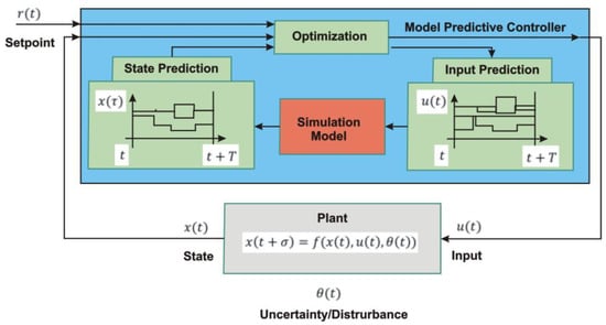
Figure 1.
Block diagram of a model predictive controller (MPC) in a feedback loop with a plant.
A process model is used to predict the current values of the output variables. The residuals, the differences between the actual and predicted outputs, serve as the feedback signal to a prediction block. The predictions are used in two types of MPC calculations that are performed at each sampling instant: set-point calculations and control calculations. Note that the MPC configuration is similar to both the internal process model control configuration and the predictor configuration because the model acts in parallel with the process and the residual serves as a feedback signal.
Expected effects of using the control algorithm (solenoid valve system) optimizing the parameters of the fuel–air mixture preparation process:
- Calorific value of combusted biogas above MWd =18 MJ/m3N;
- Electrical efficiency [ɳe], thermal efficiency [ɳt].
The current value of the parameter—ɳe = 21%, (for the current system without automatic calibration of the control object models in real-time).
The target value of the parameter—ɳe = 42% and ɳt = 50% (for a new system using the automatic calibration of models in real-time in the context of stabilization and optimization of technological processes).
- Fuel utilization efficiency (FUE)—current value of the parameter (ɳ = 40%); target value (ɳ = 90%).
Due to the dynamic changes in the production of biogas in the waste bed (temperature, humidity, compression), the current method of biogas monitoring does not ensure the preparation of its optimal parameters for use in a cogeneration unit. This condition means that some wells can be exploited with a high oxygen content, which in the long-term will require their temporary shutdown in order to return to the methanogenic phase. Energy losses result directly from the reduced overall efficiency of the cogeneration unit, determined by the non-optimal elemental composition and calorific value.
For the established operating conditions of the cogeneration unit, an increase in the energy coefficients of the cogeneration system operation can be sought only through the optimization of the preparation of the fuel–air mixture.
The task of optimizing the fuel–air mixture processes from biogas is to maximize the objective function, defined in terms of a general relationship:
where —denotes the dimension vector (number of landfill biogas streams involved in forming the fuel mixture with components , denoting the calorific values of the fuel components. The optimization process is therefore reduced to a linear programming task (linear objective function and linear constraints) with constraints (relation 1) imposed on the decision variables, defined by vector , with components , thus determining the set of admissible solutions. Since the solution to the linear programming task is only at the vertex of a feasible solution set, the search method searches the vertices (in the feasible solution region). However, this is not a complete search but a greedy strategy using a modified simplex algorithm [14,15].
A modification of the classical simplex algorithm consists of changing the system of constraint equations by adding additional equations, allowing for the analysis of changes in the decision variables, expressed in vector within the defined ranges, defined by the equation:
The objective function expressed in the general form (5) can be written as follows:
or in matrix notation
representing a one-dimensional matrix (vector of the left-hand sides of constraint equations) of the dimension of , so that the components represent the minimum content of harmful substances, while
represents a one-dimensional matrix (vector of the left-hand sides of constraint equations) of the dimension of, , so that the components represent the maximum content of harmful substances. The meaning of the individual components of the vector is analogous to . The revised simplex algorithm finds the optimal solution by examining a sequence of points in the feasible region—the region of the n-dimensional space whose points satisfy the systems of inequalities and . The principle of the algorithm is based on the observation that the solution that maximizes the objective function is located at some extreme point or vertex of the feasible region. The algorithm proceeds to a sequential search of the vertices, delimiting the feasible region until further correction of the value of the objective function is no longer possible [16,17].
Figure 2 presents a block diagram of the simplex algorithm.
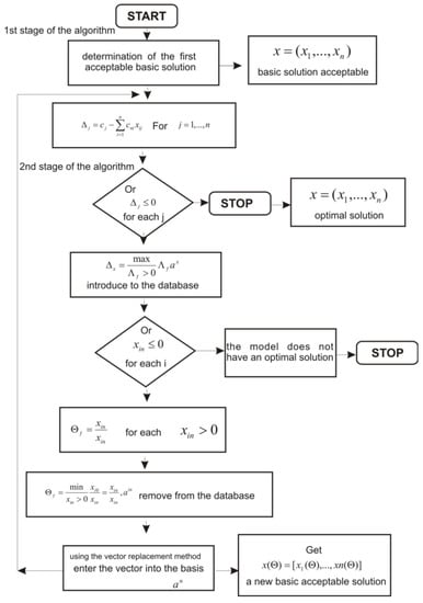
Figure 2.
Block diagram of the simplex algorithm [own work].
The principle of the algorithm is based on the observation that the solution that maximizes the objective function is located at some extreme point or vertex of the feasible region. The algorithm proceeds to a sequential search of the vertices, delimiting the feasible region until further correction of the value of the objective function is no longer possible.
Solving a linear programming problem involves the existence of the following options:
- There is one constrained solution (the objective function takes the smallest value at one vertex of the set of feasible solutions).
- There is an unconstrained solution (where the objective function can assume an arbitrarily small value while not violating the constraints).
- There are infinitely many solutions (there are at least two vertices of the set of feasible solutions where the function takes the same minimum value).
- There is no solution (i.e., the set of feasible solutions is an empty set).
This issue can be solved in polynomial or exponential time [18,19].
2.2. Implementation of the Simplex Method
In order to implement the simplex method for solving linear programming tasks, the TMetSimplex class was defined. In the public part of this class, two methods corresponding to the algorithms of the one-phase and two-phase simplex method, namely, MetSimlex and DwufazMetSimplex, were defined. In contrast, the following methods were defined in the declaration of the private section:
WartoscMinElemW is used to search for the minimum value in the preset row of the FMSmplx simplex matrix to determine the index of the independent variable, which becomes the basic variable in the next step of the algorithm. LokalizujElementBazowy is used to determine the index of the basic variable that is leaving the basis and becomes the independent variable in the next step of the algorithm. The ModyfikacjaTablicySimpleksowej implements the FMSmplx simplex matrix transformation [20,21]. Figure 3 illustrates the main form of an application, which is a computer implementation of the Pascal procedure, based on the revised simplex method.
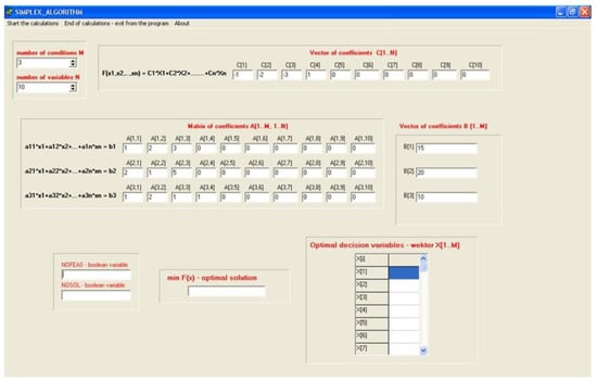
Figure 3.
Main form of the SIMPLEX_ALGORITHM application.
A class of objects for determining the minimum of a linear function with N variables passed via a constructor parameter using the simplex method has been defined in general class TMetSimplex (see Appendix A).
A procedure call in high-level language source pseudocode is shown in the following notation:
MinFunMetSimplex.DwuFazMetSimplex (list of current parameters) in the case of a two-phase simplex method for solving linear programming problems or MinFunMetSimplex.MetSimplex (list of current parameters) in the case of a simplex method for a linear programming task formulated in canonical form. The current parameter of the aforementioned class methods is an array-type variable whose components are an M-item list of the numbers of the basic variables defined in the revised simplex method.
A complex multi-threaded process control algorithm, embedded in a freely Programmable Logic Controller (supervised by a SCADA system), performs the task of solving the optimization problem, defined in the form of a neural classifier model (SVM network—support vector machine) of biogas streams, where it reproduces predefined class patterns—subsets generated by a greedy set cover approximation algorithm containing components described by a set of characteristics (including physical and chemical properties, fuel properties, and emissions). Each subset—representing the model class—is the result of optimization using the greedy set cover approximation algorithm, maximizing the objective function (calorific value—MWd) while satisfying the process and technological criteria imposed on the decision variables of the linear programming task. The model classes are described by a set of features, which allows an algorithm at a lower level of technological process control to perform classification using the SVM network model (MC SVM) based on a set of features assigned to predefined class patterns, represented by disjoint subsets of the coverage generated by the greedy set cover master algorithm, and finally, to check whether the identified component belongs to the class pattern by an incidence matrix [22,23].
2.3. Mathematical Model of the MC SVM Neural Classifier Algorithm
The classification uses the MC SVM classifier (multi-class support vector machine), based on a unidirectional neural network implementing different types of activation functions including linear, polynomial, radial, and sigmoid functions. The task of classification consists of maximizing the margin of separation between two different classes described by a set of pairs where xi is the input vector and di is the setpoint (for two classes, it reaches a value of 1 for class 1 or −1 for class 2) [24,25]. Assuming linear separability of the two classes, the equation of the hyperplane separating the two classes can be written as:
where , .
In this equation, assuming , inputs, the weight vector is N-dimensional. The weight is polarization. The decision equations determining class membership take the form of:
or, after transformations,
If a pair of points (xi, di) satisfies the above equation with an equal sign, then the vector forms a so-called support vector. Support vectors are those data points that lie closest to the optimal hyperplane and are the hardest to classify.
The problem of training linear SVM networks (i.e., the selection of synaptic connection weights for linearly separable training data) comes down to maximizing the separation margin. This is a quadratic programming problem with linear constraints on the weights, which is solved using the method of Lagrange multipliers by minimizing the so-called Lagrange functions.
Considering that the training task comes down to the maximization of the Lagrange functions relative to the Lagrange multipliers, the primal problem transforms into a dual problem, which is formulated as follows:
with the following constraints:
Solving the above optimization problem with respect to the Lagrange multipliers allows one to determine the equation of the optimal hyperplane, defined by the weight vector and the polarization parameter .
When solving the problem of classifying non-linearly separable patterns, the problem comes down to determining the optimal hyperplane that minimizes the likelihood of a classification error on the training set with the widest possible separation margin.
As is the case with linearly separable patterns, the primal problem is reduced to a dual problem, which is formulated as follows:
with the following constraints:
for i = 1, 2, …, p and the constant value C adopted by the user. Thus, from the solution of the dual problem, one obtains the expression for the vector of weights of the optimal hyperplane in the form of
The optimal hyperplane equation depends solely on the support vectors. The other vectors from the training dataset have no impact on the solution result.
The equation defining the output signal of the linear SVM network with optimal weights is expressed by the following relationship
The primal problem is solved by its transformation into a dual problem, identical to that for networks with linear pattern separability by minimizing the Lagrange functions.
In the first stage, the solution to this optimization problem assumes a comparison to zero of the partial derivatives of the Lagrange functions with respect to w, b, and .
The primal problem transforms into a dual problem defined relative to the Lagrange multipliers in the following form
with the following constraints
The function present in the formulated dual task is the scalar product of the vector function
Due to the classification problem requiring the separation of data into a larger number of classes, multiple classifications are required using the “one-against-all” and “one-against-one” methods. In the one-against-all method (Algorithm 1) with M classes, MC SVM networks recognizing exactly one class are defined. This method requires the training of M SVM networks, each on a different dataset [26,27]. Once all M networks have been trained, a reproduction step follows, in which the same vector x is fed to each SVM network and the output signals (M decision functions) of all trained SVM networks are determined.
| Algorithm 1: Definition of the MC SVM algorithm. |
| Input: Category N, inputfor training samples; testing sample T. |
| Output: Categories of T. |
| Algorithm: |
| 2: for n = 1 to N |
| 3: Positive Sample ← , Negative Sample ← other samples except |
| 4: Store the data of classifier |
| 5: end for |
| 7: for n = 1 to N |
| 8: Use classifier to calculate the value of |
| 9: end for |
| 10: Compare all , output the n corresponding to the maximum of |
The SVM network was chosen for the pattern classification task because of its generalization capabilities. The SVM network is marginally sensitive to the chosen learning hyperparameters determining the number of neurons in the hidden layer. Due to the need to increase the quality index of the technological process control in cogeneration plants, in the context of obtaining products with precisely defined physicochemical, combustible and emission properties, the SVM algorithm was modified by expanding the library of basic class patterns to include a library of predefined class patterns described by physicochemical and combustible properties (calorific value, humidity).
The master algorithm (i.e., the greedy set cover approximation algorithm) is responsible for generating class patterns corresponding to optimized disjoint subsets of the set whose elements are biogas streams. The model classes are described by a set of features, which allows an algorithm at a lower level of process control to perform classification using the SVM network model (MC SVM) based on a set of features assigned to predefined class patterns, represented by disjoint subsets of the coverage generated by the greedy set cover master algorithm [28,29].
2.4. Method for Solving the Greedy Set Cover Optimization Problem
The parameter for this method is the pair , consisting of a finite set X (the set of biogas streams) and a family F of subsets of X (corresponding to predefined class patterns defined based on the fuel and physicochemical properties and satisfying the criterion of the formulated objective function (i.e., ), so that each element of the set X belongs to at least one subset of the family F: In this case, the subset , covers its elements. The solution of the method is the subfamily , whose elements cover the entire set X: .
The listing given is a (pseudocode) implementation of the GREEDY-SET-COVER Algorithm 2, which works as follows. In each phase, U stands for the set of elements not yet covered. The set , includes the coverage being constructed. Line 4 is the stage at which a greedy decision is taken (i.e., a subset S that covers as many of the uncovered elements (fraction components) as possible is selected). Once S has been selected, its elements are removed from U and S itself is added to . When the algorithm terminates, the set is a subfamily of F, covering X.
| Algorithm 2: Greedy Set Cover |
| 1. |
| 2. |
| 3. while |
| 4. do choose that maximizes |
| 5. |
| 6. |
| 7. return |
The mathematical model for the optimization of the process of light fraction production (the so called calorific fraction), consisting of the separation (in the optical sorter(s)) from the heavy oversize fraction waste stream of non-metallic components with high calorific value MWd, is represented by the matrix (column vector).
Z = (z_j) with components storing indices of model classes corresponding to the subsets of coverage of the set.
P^k = (p_ij) generated by the greedy set cover optimization algorithm, with components p_ij containing the i-th component (fraction) contained in the waste stream directed to the optical sorter in the j-th model class.
The number of predefined model classes is determined by the number of optimal subsets found by the greedy set cover algorithm (i.e., the greedy set cover) approximation algorithm for covering optimal subsets P^k, which satisfy the criterion:
The master algorithm of the SVM checks in each iteration whether the identified (based on the analysis of spectroscopic spectra) component/fraction belongs to a model class defined on the basis of fuel and physicochemical properties and compliance with the criterion of the formulated objective function.
In summary, the algorithm implemented in the control layer of the optimizing SCADA system must reproduce the predefined model class patterns (i.e., greedy set cover-generated subsets containing components in the form of biogas streams), described by a set of characteristics including the physicochemical properties, fuel properties, and the MWd [30,31,32].
The SCADA data visualization, control, and archiving system for the municipal waste landfill was developed (i.e., in particular, measuring devices were installed to monitor the concentration of methane and oxygen in biogas from individual wells in the cogeneration system in order to automate the regulation of the power of the cogeneration unit based on the concentration of methane and oxygen in biogas). The following elements were installed individually at each well entrance in the collective collector:
- Regulating gas solenoid valve with a step head;
- Solenoid valve for biogas sampling;
- Manual shut-off gas valve;
- Rotameter;
- Measuring port.
Each of the collecting stations was equipped with a control cabinet with a system for regulating, controlling, and visualizing the process. Additionally, a stationary biogas analyzer was installed at each station that continuously measured the two biogas parameters (CH2 and O2) for each connection in the gas manifold. The measurement results of these two parameters showed a partial reduction in the biogas stream through the solenoid valve in the case of a methane content below the assumed threshold or an increase in the biogas stream flow in the case when the CH4 value is higher than the assumed level. A similar situation will also apply to the content of O2. In extreme cases, the control system turns off gas wells whose parameters differ from those assumed in the algorithm.
Figure 4 presents a hierarchical control system optimizing the composition of the fuel mixture.
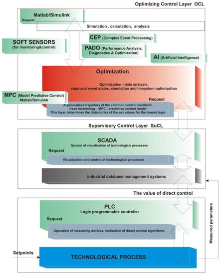
Figure 4.
Hierarchical control system optimizing the composition of the fuel mixture.
3. Results and Discussion
Landfilling of municipal waste is a common process in most countries. In this technology, the key is the acquisition and disposal of landfill gas generated in the waste deposit. The approach proposed in the work at the research facility concerns the acquisition of landfill gas with the use of degassing wells and its conversion, in order to generate energy. The presented solution implements two main aspects of sustainable development (i.e., it reduces the emissions of greenhouse gases from landfill (methane and carbon dioxide)) and uses landfill gas as a source of renewable energy. Such solutions mean that the landfill significantly reduces its negative impact on individual components of the environment.
3.1. A Case Study
3.1.1. Characteristics of the Object of Study
The municipal landfill covers an area of 34,000 m2. The operation of the currently active landfill has been divided into four phases:
- PHASE I (Quarter I)—with an area of 3.3 hectares, used in the 2000–2008 period;
- PHASE II (Quarter II)—with an area of about 3.9 hectares, used in the 2008–2012 period;
- PHASE IV (Quarter IV)—with an area of about 3.2 hectares, used in the 2013–2018 period;
- PHASE III (Quarter III)—with an area of about 4.0 hectares, currently in use.
The storage technology consists of depositing the waste in stages by filling the waste chamber layer by layer. The area used measures 30 × 50 m, with an unloading platform measuring 20 ÷ 30 m in width, and is shifted successively to areas not yet filled with waste. The waste is delivered to the active chamber by truck via a network of temporary roads and is then placed into storage layers and pre-compacted with a bulldozer. Once a layer has been laid, a compactor is used to compact the waste. The thickness of one layer after compaction does not exceed 1.8 m. Once a layer of compacted waste has been formed, a transfer layer measuring about 0.20–0.30 m and made of inert materials is also created [33,34].
The landfill gas produced in the waste deposit is treated and used as fuel for the gas engine in the CHP system. The biogas conditioning installation contains elements to improve the quality of biogas (i.e., a drying station, a carbon filter, and technology consisting of a fixed-bed reactor with simultaneous regeneration of the bed with oxygen). The implemented solution allows for optimization of the LFG composition to ensure the reliability of the power generation process and reduce the gas and dust emissions into the environment [35].
3.1.2. Model Validation
To simulate the fuel mixture formation process and assess the model’s compatibility with the real process, a dedicated application was developed based on the component models presented in the previous sections. The following assumptions were made for this purpose:
- Five biogas streams from degassing wells with the parameters specified in Table 1 were used to form the fuel mixture (Table 1).
 Table 1. Biogas stream composition of components G1–G5.
 - The criteria imposed on the process parameters are shown in Table 2.
Table 2. Constraints for the optimization procedure.
The computer simulations and online measurements showed very good agreement between the developed model and the real process, as follows, respectively:
- For the proportion of
- For the proportion of ;
- For the calorific value of gas mixture .
The root mean square error (RMSE):
where
—is a calculated quantity;
—measured quantity;
—number of measurements.
The use of the modified simplex algorithm in the fuel mixture formation process made it possible to determine the optimum values for the proportions of the individual fuel components (range of variation: no biogas collection—regenerated well), (range of variation: no biogas collection—regenerated well), (range of variation: no biogas collection—regenerated well), (range of variation: 0.28–0.58), (range of variation: 0.42–0.72) with the following constraints set for the decision variables of the task:
, where denote the proportion of in the fuel mix, and , where denote the proportion of in the fuel mix, while , and , , respectively, are the permissible values of the proportions of f and in the formed component of the fuel mixture and ). The optimum value of the objective function of the formed fuel mixture component was in the following range: 16.2–19.3 .
The computer simulation results differed only slightly from the data measured online, confirming the high agreement of the model with the real process.
3.2. Analysis of Simulation Results
The effect of a particular gaseous fuel on the operation of a reciprocating internal combustion engine depends primarily on its physical and chemical properties. Among the most relevant fuel parameters are its elemental composition, calorific value, density, minimum air demand for combustion, flammability limits, and methane number value [36,37]. The chemical composition directly affects the calorific value of the fuel–air mixture. In turn, the calorific value of the combustible mixture has a decisive influence on the amount of mechanical work generated by the engine at a given speed (i.e., its power output) [38,39]. The analysis of the theoretical cycle indicated that the air excess ratio and the composition of the gaseous fuel (biogas) being combusted significantly affect the efficiency and work per unit of the thermodynamic cycle and, consequently, the performance of the actual internal combustion engine [40,41]. It should be borne in mind that in real operating conditions, other physical phenomena occur, which will play an important role in shaping the efficiency curve and effective unit operation of the actual internal combustion engine [42,43].
The algorithm controlling the operation of the solenoid valves implements/follows the reference trajectory of the demand/consumption of gaseous fuel by the internal combustion engine of the CHP unit. A change in the gas parameters in the degassing well G1–G5 (see the parameters of biogas in Table 1) causes an event of a change in the well’s operating state and the detection system of these changes calls the method in response—a sequence of simplex, MC SVM, and greedy set cover (master algorithm) algorithms and sets the value of the signal supplied by the PLC to the actuators (i.e., solenoid valves (open/close level)). As a result, the control algorithm stabilizes the engine operation by reproducing the theoretical (as a reference) OTTO cycle, determining the optimal composition of the fuel–air mixture based on the determined shares of streams of individual degassing wells, taking into account their operating characteristics and operating states (operating transmittances).
The automatic control system is based on a freely programmable PLC controller, in which a control algorithm has been implemented that follows the reference trajectory of methane and oxygen concentrations, which allows to obtain (with the current and predicted biological activity of the bed deposited at the landfill) the calorific value of the combusted biogas above 18 MJ/m3N.
The annual energy effect was obtained after the modernization of the fuel mixture preparation system, in particular:
- -
- Electric energy gross generated in the bio power plant after modernization—248.00 MWh (vs. 135.35 MWh before modernization).
Increased efficiency of the cogenerator cycle and the fuel preparation system:
- -
- Electrical efficiency [ɳe], thermal efficiency [ɳt];
The current value of the parameter—ɳe = 42%;
The current value of the parameter—ɳt = 50%;
- -
- Fuel utilization efficiency (FUE)—current value of the parameter (ɳ = 90%).
This solution implements modern energy technologies in the landfill in order to improve the efficiency of the use of renewable energy sources and reduce the negative impact of the landfill on the environment.
3.3. Innovative Methods of Solving a Research Problem
- A.
- In the field of ICT solutions and control systems.
A complex multi-threaded technological process control algorithm (goal: stabilization of the fuel–air mixture composition) was built into a freely programmable logic controller PLC (supervised by the SCADA system) to perform the task related to solving the optimization problem, defined in the form of a neural classifier model (SVM network—support vector machine) of components of biogas streams from individual degassing wells where it recreates patterns of predefined classes—subsets generated by the greedy set cover approximation algorithm containing components described by a set of features (including physical and chemical properties, fuel properties). Each subset—representing the model class of components—forming the fuel mixture is the result of optimization using the greedy set cover greedy approximation algorithm, maximizing the objective function (MWd calorific value) while meeting the process and technological constraints imposed on the decision variables of linear programming tasks (humidity, H2S share). Reference classes are described by a set of features, which allows the algorithm at a lower level to control the process of mixing biogas streams to classify using the SVM network model (MC SVM) based on a set of features assigned to predefined class patterns, represented by disjoint coverage subsets generated by the superior greedy set cover algorithm and finally check whether the identified component belongs to the class pattern by the incident matrix.
- B.
- In terms of technological solutions for the biogas and energy system (waste deposit degassing installation, biogas container collecting stations, blower station, biofilter, flare, integrated cogeneration unit).
The SCADA data visualization, control, and archiving system for the municipal waste landfill was developed (i.e., in particular, measuring devices were installed to monitor the concentration of methane and oxygen in biogas from individual wells in the cogeneration system in order to automate the regulation of the power of the cogeneration unit based on the concentration of methane and oxygen in biogas).
The following elements were installed individually at each well entrance in the collective collector:
- Regulating gas solenoid valve with a step head;
- Solenoid valve for biogas sampling;
- Manual shut-off gas valve;
- Rotameter;
- Measuring port.
Each of the collecting stations was equipped with a control cabinet with a system for regulating, controlling, and visualizing the process. Additionally, a stationary biogas analyzer was installed at each station that continuously measured two biogas parameters (CH2 and O2) for each connection in the gas manifold. The measurement result of these two parameters resulted in a partial reduction of the biogas stream through the solenoid valve in the case of a methane content below the assumed threshold or an increase in the biogas stream flow in the case when the CH4 value is higher than the assumed level. A similar situation will also apply to the content of O2. In extreme cases, the control system turns off gas wells whose parameters differ from those assumed in the algorithm.
4. Conclusions
The maximum efficiency of cogeneration systems mainly depends on the stable operation of the internal combustion engine, determined by the calorific value of the air–fuel mixture in the engine cylinders. The impact of gaseous fuel (landfill biogas) on the operation of a piston internal combustion engine in a cogeneration system depends primarily on its physical and chemical properties. The most important fuel parameters include the elemental composition, calorific value, minimum combustion air requirement, flammability limits, and methane number value. The elemental composition directly affects the calorific value of the fuel–air mixture. In turn, the calorific value of the combustible mixture has a decisive influence on its power and torque. The performance of the internal combustion engine, expressed in terms of torque and effective power at a specific rotational speed, depends to a large extent on the parameters of the fuel–air mixture. In spark-ignition engines, quantitative regulation of the composition of the gas–air mixture is used. This type of regulation consists of throttling the amount of air supplied to the internal combustion engine depending on its load. According to the amount of air, gas is supplied to the cylinder in an amount ensuring engine operation with the required ratio of excess air λ. The optimal ratio of the amount of fuel to air when feeding the internal combustion engine allows one to obtain the expected effective power with the lowest possible fuel consumption.
The authors solved the research problem by using the MPC predictive control model generating optimal sequences of the control decisions—control trajectories of actuators (i.e., solenoid valves regulating biogas streams sucked from individual biogas intake wells from the landfill waste deposit) and a throttle regulating the stream of fuel supplied to the engine on the basis of signals received from the process model (i.e., obtained by solving the model written in the form of state equations by updating, optimizing the matrix of state variables, and minimizing the objective function defined as minimizing the error of following the reference trajectory of control signals u(t)—vector of control variables at a given moment (i.e., with the adopted control horizon and prediction horizon).
The model of the MPC predictive control algorithm was implemented in a SCADA type hierarchical optimizing control system using a freely programmable PLC controller, which was tested using the Siemens TIA Portal-PLC Sim Advanced V4.0 software.
The annual energy effect was obtained after the modernization of the fuel mixture preparation system (i.e., in particular, electric energy gross generated in the bio power plant after modernization was 248.00 MWh (vs. 135.35 MWh before modernization)).
Increased efficiency of the cogenerator cycle and the fuel preparation system.
- -
- Electrical efficiency [ɳe], thermal efficiency [ɳt].
The current value of the parameter—ɳe = 42%;
The current value of the parameter—ɳt = 50%.
- -
- Fuel utilization efficiency (FUE)—current value of the parameter (ɳ = 90%).
Author Contributions
Conceptualization, K.G., A.G. and K.C.; Methodology, K.G. and I.W.; Software, K.G., A.G. and J.C.; Validation, K.G., A.G.-C. and P.K.; Formal analysis, K.G., A.G., J.C., I.W., P.K. and M.M.; Investigation, K.G., A.G.-C., J.C. and M.M.; Resources, K.G., A.G. and A.G.-C.; Data curation, K.G., A.G.-C., J.C., P.K. and K.C.; Writing—original draft, K.G., A.G., A.G.-C. and K.C.; Writing—review & editing, A.G., A.G.-C. and K.C.; Visualization, M.M.; Supervision, K.G. and I.W.; Project administration, A.G. All authors have read and agreed to the published version of the manuscript.
Funding
This research received no external funding.
Data Availability Statement
Not applicable.
Conflicts of Interest
The authors have no conflict of interest.
Appendix A. A Source Code Declaration of TMetSimplex Class of Objects for Determining the Minimum of a Linear Function with N Variables Passed via a Constructor Parameter Using the Simplex Method
| TMetSimplex = class // A class of objects for determining the minimum of a linear function with N variables passed via a constructor parameter using the simplex method private FMSmplx : TMacierzF; // Simplex matrix with the dimensions [0..M + 1,0..N + 1] FN, FM, Fmaxit : Integer; // N– number of task variables, M–number of constraint equations FJestWynik : boolean; FWekX :TMacierzF; // WekX–solution vector Feps,FminF :TFloat; // eps–accuracy of differentiation of the zero element minF–the calculated minimum of the function F(WekX) function Result:TFloat; procedure WartoscMinElemW( NrW : Integer; LstKol : TMacierzI; LeLK : Integer; WBzw : Boolean; var IKol : Integer; var WMin : TFloat); // Determination, in the row number NrW of the simplex matrix MSmplx.A, of the number of the independent variable that will become the basic variable–step 2a of the algorithm LstKol - list of feasible column numbers; LeLK–number of elements in the list LstKol; WBzw–method of determining the minimum value: whether as an arithmetic difference or as a difference of absolute values; IKol–determined index of the column with the minimum value WMin; WMin–determined minimum value procedureLokalizujElementBazowy( LstWrs : TMacierzI; LeLW : Integer; var IWrs : Integer; NrK : Integer; var Qb : TFloat); // Searching for the number of the basic variable leaving the basis based on the minimum value of the coefficient Q in column NrK for the preset row list; LstWrs–list of row numbers in column NrK; LeLW–number of elements in the list LstWrs; IWrs–determined index of the row with the basic element in column NrK; NrK–number of the column under analysis; Qb–minimum value of the coefficient at the basic element (taking degeneration into account) procedureModyfikacjaTablicySympleksowej( PFaza : Boolean; IWB, IKB : Integer); // Calculation of the value of the simplex matrix MSmplx.A for the selected independent variable IKB becoming the basic variable in place of the basic variable IKB becoming the independent variable; PFaza–the phase number of the method on which the number of analyzed rows of the simplex matrix depends (for phase I including M+1 rows of the ancillary task); IWB–the index of the row in which the variable leaving the base is located; IKB–the index of the column in which the new basic variable is located. public constructor Create(WekC,MacA,WekB: TMacierzF; LZm,LRw: Integer; WekY: TMacierzF; maxit1: Integer; eps1: TFloat); // Initialization of the simplex array FMSmplx.A for the input: WekC–vector of coefficients of the objective function (3.80); MacA–matrix of the system of constraint equations (3.82); WekB–non-negative vector of free expressions of this system; LZm - number of variables of the task (N); LRw–number of equations (M); WekY–vector of solution; maxit1–fixed maximum number of iterations terminating the calculation; eps1–accuracy of distinguishing zero element function DwuFazMetSimplex:Integer; // Two-phase simplex method for solving a linear programming task // Result–error number; Result=0–no error function MetSimplex(LstZmBaz: TmacierzI):Integer; // The simplex method for solving a linear programming task in the canonical form; LstZmBaz–M-item list of basic variable numbers; Result–error number; Result=0–no error property MinFun : TFloat read Result; destructor Destroy; override; end; |
References
- Ciuła, J.; Generowicz, A.; Gaska, K.; Gronba-Chyła, A. Efficiency Analysis of the Generation of Energy in a Biogas CHP System and its Management in a Waste Landfill—Case Study. J. Ecol. Eng. 2022, 23, 143–156. [Google Scholar] [CrossRef]
- Sobiecka, E. Thermal and physicochemical technologies used in hospital incineration fly ash utilization before landfill in Poland. J. Chem. Technol. Biotechnol. 2016, 91, 2457–2461. [Google Scholar] [CrossRef]
- Im, Y. Assessment of the Impact of Renewable Energy Expansion on the Technological Competitiveness of the Cogeneration Model. Energies 2022, 15, 6844. [Google Scholar] [CrossRef]
- Vakalis, S.; Moustakas, K. Applications of the 3T Method and the R1 Formula as Efficiency Assessment Tools for Comparing Waste-to-Energy and Landfilling. Energies 2019, 12, 1066. [Google Scholar] [CrossRef]
- Wysowska, W.; Wiewiórska, I.; Kicińska, A. The impact of different stages of water treatment process on the number of selected bacteria. Water Resour. Ind. 2021, 26, 100167. [Google Scholar] [CrossRef]
- Nguyen, Q.T.; Le, M.D. Effects of Compression Ratios on Combustion and Emission Characteristics of SI Engine Fueled with Hydrogen-Enriched Biogas Mixture. Energies 2022, 15, 5975. [Google Scholar] [CrossRef]
- Den Boer, E.; Jędrczak, A. Performance of mechanical biological treatment of residual municipal waste in Poland. E3S Web Conf. 2017, 22, 00020. [Google Scholar] [CrossRef]
- Graz, K.; Kwaśny, J. Microplastics in composts as a barrier to the development of circular economy. Archit. Civ. Eng. Environ. 2021, 14, 137–144. [Google Scholar] [CrossRef]
- Ma, L.; Yu, Y. Coupling characteristics of combustion-gas flows generated by two energetic materials in base bleed unit under rapid depressurization. Appl. Therm. Eng. 2019, 148, 502–515. [Google Scholar] [CrossRef]
- Sobiecka, E.; Cedzynska, K.; Smolinska, B. Vitrification of medical waste as an alternative method of wastes stabilization. Fresenius Environ. Bull. 2010, 19, 3045–3048. [Google Scholar]
- Kowalski, S. Failure analysis of the elements of a forced-in joint operating in rotational bending conditions. Eng. Fail. Anal. 2020, 118, 104864. [Google Scholar] [CrossRef]
- Caposciutti, G.; Baccioli, A.; Ferrari, L.; Desideri, U. Biogas from Anaerobic Digestion: Power Generation or Biomethane Production? Energies 2020, 13, 743. [Google Scholar] [CrossRef]
- Novotny, V.; Spale, J.; Szucs, D.J.; Tsai, H.-J.; Kolovratnik, M. Direct integration of an organic Rankine cycle into an internal combustion engine cooling system for comprehensive and simplified waste heat recovery. Energy Rep. 2021, 7, 644–656. [Google Scholar] [CrossRef]
- Ahmed, M.Z.; Padhiyar, N. Multi objective optimization of a tri-reforming process with the maximization of H2 production and minimization of CO2 emission & power loss. Int. J. Hydrog. Energy 2020, 45, 22480–22491. [Google Scholar] [CrossRef]
- Bracco, S.; Siri, S. Exergetic optimization of single level combined gas–steam power plants considering different objective functions. Energy 2010, 35, 5365–5373. [Google Scholar] [CrossRef]
- Su, H.; Lan, F.; He, Y.; Chen, J. A modified downhill simplex algorithm interpolation response surface method for structural reliability analysis. Eng. Comput. 2020, 37, 1423–1450. [Google Scholar] [CrossRef]
- Chahal, D.; Stuart, S.J.; Goasguen, S.; Trout, C.J. Automated, Parallel Optimization of Stochastic Functions Using a Modified Simplex Algorithm. In Proceedings of the Sixth IEEE International Conference on e-Science Workshops, Brisbane, Australia, 7–10 December 2010; pp. 98–103. [Google Scholar] [CrossRef]
- Nabli, H. An overview on the simplex algorithm. Appl. Math. Comput. 2009, 210, 479–489. [Google Scholar] [CrossRef]
- Vieira, H., Jr.; Lins, M.P.E. An improved initial basis for the Simplex algorithm. Comput. Oper. Res. 2005, 32, 1983–1993. [Google Scholar] [CrossRef]
- Lalami, M.E.; Boyer, V.; El-Baz, D. Efficient Implementation of the Simplex Method on a CPU-GPU System. In Proceedings of the IEEE International Symposium on Parallel and Distributed Processing Workshops and Phd Forum, Anchorage, AK, USA, 16–20 May 2011; pp. 1999–2006. [Google Scholar] [CrossRef]
- Huangfu, Q.; Hall, J.A.J. Parallelizing the dual revised simplex method. Math. Prog. Comp. 2018, 10, 119–142. [Google Scholar] [CrossRef]
- Nannicini, G. Fast Quantum Subroutines for the Simplex Method. In Integer Programming and Combinatorial Optimization. IPCO 2021. Lecture Notes in Computer Science; Singh, M., Williamson, D.P., Eds.; Springer: Cham, Germany, 2021; Volume 12707. [Google Scholar] [CrossRef]
- Stojković, N.V.; Stanimirović, P.S.; Petković, M.D. Modification and implementation of two-phase simplex method. Int. J. Comput. Math 2009, 86, 1231–1242. [Google Scholar] [CrossRef]
- Rocco, C.M.S.; Zio, E. A support vector machine integrated system for the classification of operation anomalies in nuclear components and systems. Reliab. Eng. Syst. Saf. 2007, 92, 593–600. [Google Scholar] [CrossRef]
- Lu, G.; Zhang, H.; Sha, X.; Chen, C.; Peng, L. TCFOM: A Robust Traffic Classification Framework Based on OC-SVM Combined with MC-SVM. In Proceedings of the International Conference on Communications and Intelligence Information Security, Xi’an, China, 13–14 October 2010; pp. 180–186. [Google Scholar] [CrossRef]
- Wiśniewski, R.; Bazydło, G.; Szcześniak, P. SVM algorithm oriented for implementation in a low-cost Xilinx FPGA. Integration 2019, 64, 163–172. [Google Scholar] [CrossRef]
- Xu, H.; Bie, X.; Feng, H.; Tian, Y. Multiclass SVM active learning algorithm based on decision directed acyclic graph and one versus one. Clust. Comput. 2019, 22, 6241–6251. [Google Scholar] [CrossRef]
- Guerrero, M.C.; Parada, J.S.; Espitia, H.E. EEG signal analysis using classification techniques: Logistic regression, artificial neural networks, support vector machines, and convolutional neural networks. Heliyon 2021, 7, e07258. [Google Scholar] [CrossRef]
- Meng, J.L.Q.; Zhang, G.; Sun, Y.; Qiu, L.; Ma, W. Automatic modulation classification using support vector machines and error correcting output codes. In Proceedings of the IEEE 2nd Information Technology Networking, Electronic and Automation Control Conference (ITNEC), Chengdu, China, 15–17 December 2017; pp. 60–63. [Google Scholar] [CrossRef]
- Elomaa, T.; Kujala, J. Covering Analysis of the Greedy Algorithm for Partial Cover. In Algorithms and Applications. Lecture Notes in Computer Science; Elomaa, T., Mannila, H., Orponen, P., Eds.; Springer: Berlin/Heidelberg, Germany, 2010; p. 6060. [Google Scholar] [CrossRef]
- Cui, P. A Tighter Analysis of Set Cover Greedy Algorithm for Test Set. In Combinatorics, Algorithms, Probabilistic and Experimental Methodologies; ESCAPE 2007. Lecture Notes in Computer Science; Chen, B., Paterson, M., Zhang, G., Eds.; Springer: Berlin/Heidelberg, Germany, 2007; p. 4614. [Google Scholar] [CrossRef]
- Yang, Y.; Xin, Y.; Zhi-Hua, Z. On the approximation ability of evolutionary optimization with application to minimum set cover. ArtifIntell 2012, 180–181, 20–33. [Google Scholar] [CrossRef]
- Ciuła, J. Analysis of the effectiveness of wastewater treatment in activated sludge technology with biomass recirculation. Archit. Civ. Eng. Environ. 2022, 15, 123–134. [Google Scholar] [CrossRef]
- Gronba-Chyła, A.; Generowicz, A.; Kwaśnicki, P.; Cycoń, D.; Kwaśny, J.; Grąz, K.; Gaska, K.; Ciuła, J. Determining the Effectiveness of Street Cleaning with the Use of Decision Analysis and Research on the Reduction in Chloride in Waste. Energies 2022, 15, 3538. [Google Scholar] [CrossRef]
- Rasi, S.; Veijanen, A.; Rintala, J. Trace compounds of biogas from different biogas production plants. Energy 2007, 32, 375–1380. [Google Scholar] [CrossRef]
- Ajhar, M.; Travesset, M.; Yüce, S.; Melin, T. Siloxane removal from landfill and digester gas—A technology overview. Bioresour. Technol. 2010, 101, 2913–2923. [Google Scholar] [CrossRef]
- Smol, M.; Włodarczyk-Makuła, M. Effectiveness in the Removal of Organic Compounds from Municipal Landfill Leachate in Integrated Membrane Systems: Coagulation—NF/RO. Polycycl. Aromat. Compd. 2017, 37, 456–474. [Google Scholar] [CrossRef]
- Tappen, S.J.; Aschmann, V.; Effenberger, M. Lifetime development and load response of the electrical efficiency of biogas-driven cogeneration units. Renew. Energ. 2017, 114, 857–865. [Google Scholar] [CrossRef]
- Ciuła, J.; Kowalski, S.; Wiewiórska, I. Pollution Indicator of a Megawatt Hour Produced in Cogeneration—the Efficiency of Biogas Purification Process as an Energy Source for Wastewater Treatment Plants. J. Ecol. Eng. 2023, 24, 232–245. [Google Scholar] [CrossRef]
- Piechota, P.; Synowiec, P.K.; Andruszkiewicz, A.; Wędrychowicz, W. Selection of the Relevant Turbulence Model in a CFD Simulation of a Flow Disturbed by Hydraulic Elbow—Comparative Analysis of the Simulation with Measurements Results Obtained by the Ultrasonic Flowmeter. J. Therm. Sci. 2018, 27, 413–420. [Google Scholar] [CrossRef]
- Khalid, M.B.; Beithou, N.; Al-Taani, M.A.S.; Andruszkiewicz, A.; Alahmer, A.; Borowski, G.; Alsaqoor, S. Integrated Eco-Friendly Outdoor Cooling System—Case Study of Hot-Humid Climate Countries. J. Ecol. Eng. 2022, 23, 64–72. [Google Scholar] [CrossRef]
- Thomas, M.; Kozik, V.; Barbusiński, K.; Sochanik, A.; Jampilek, J.; Bąk, A. Potassium Ferrate (VI) as the Multifunctional Agent in the Treatment of Landfill Leachate. Materials 2020, 13, 5017. [Google Scholar] [CrossRef]
- Dalpaz, R.; Konrad, O.; Cândido da Silva, C.C.; Barzotto, H.P.; Hasan, C.; Guerini, F.M. Using biogas for energy cogeneration: An analysis of electric and thermal energy generation from agro-industrial waste. Sustain. Energy Technol. Assess. 2020, 40, 100774. [Google Scholar] [CrossRef]


Disclaimer/Publisher’s Note: The statements, opinions and data contained in all publications are solely those of the individual author(s) and contributor(s) and not of MDPI and/or the editor(s). MDPI and/or the editor(s) disclaim responsibility for any injury to people or property resulting from any ideas, methods, instructions or products referred to in the content. |
© 2023 by the authors. Licensee MDPI, Basel, Switzerland. This article is an open access article distributed under the terms and conditions of the Creative Commons Attribution (CC BY) license (https://creativecommons.org/licenses/by/4.0/).