Numerical Simulation and Experimental Investigation of Variable Mass Flow in Horizontal Wellbores: Single-Phase and Multiphase Analysis


1
Petroleum Exploration and Production Research Institute of SINOPEC, Beijing 100083, China
2
State Key Laboratory of Shale Oil and Gas Enrichment Mechanisms and Effective Development, Beijing 100083, China
3
Sinopec Key Laboratory of Shale Oil/Gas Exploration and Production Technology, Beijing 100083, China
4
Petroleum Engineering Institute, Yangtze University, Wuhan 430100, China
5
Key Laboratory of Drilling and Production Engineering for Oil and Gas, Wuhan 430100, China
*
Author to whom correspondence should be addressed.
Energies 2023, 16(16), 6073; https://doi.org/10.3390/en16166073
Submission received: 17 July 2023
/
Revised: 16 August 2023
/
Accepted: 17 August 2023
/
Published: 19 August 2023
(This article belongs to the Section H1: Petroleum Engineering)
Abstract
:Considering the current limitations and restricted scope of existing experiments, as well as the absence of corresponding numerical simulation verifications and comparisons, and the lack of actual case studies of variable mass flow calculation and comparison, this study focuses on high production oilfields in the Mideast and South China Sea. The objective is to investigate single-phase and multiphase variable mass flow through numerical and experimental simulations. The study develops linear regression equations to establish the relationship between the mixture pressure drop caused by side flow and the velocities of the main flow, as well as the ratio between side and main flow velocities. Actual calculations using these equations are provided. The comprehensive analysis reveals that, for a fixed total flow rate, an increase in the side versus main injection velocity ratio leads to an increase in pressure loss before and after the injection hole. In single-phase flow, the friction factor for side hole flow is generally higher than that for only axial main flow, with the same total flow rate. In multiphase flow, when the gas-liquid ratio (GLR) is relatively large, the side flow has minimal impact on pressure drop, while at lower GLR values, the side flow significantly increases the pressure drops. When predicting the pressure drop for single-phase variable mass flow in horizontal wellbores, it is appropriate to consider only the mixture pressure drop caused by the closest hole to the calculation section, assuming the injection hole flow rates are approximately equal. In terms of predicting the productivity of single-phase variable mass flow, it is crucial to consider the mixture pressure drop. Neglecting the mixture pressure drop can lead to relatively larger productivity prediction results, with potential production rate errors exceeding 50%. The accuracy of the prediction is influenced by the ratio of mixture pressure drop to production pressure differential, and the pressure along the external zone of the screen pipe is higher when considering the mixture pressure drop compared to when it is neglected. Additionally, the flow rate along the external zone of the screen pipe becomes more non-uniform when the mixture pressure drop is considered. Furthermore, the findings from the single-phase and multiphase flow experiments suggest that significant deviations in production rates may occur in scenarios with low gas-liquid ratio (GLR), highlighting the need for further investigation in this area.
1. Introduction
Over the past three decades, studies have consistently shown that considering horizontal wellbore pressure drop is crucial for accurately predicting the productivity of horizontal wells, especially those with high permeability formations, high production rates, and long horizontal wellbore. In earlier studies conducted before the 1990s, the pressure drop of horizontal wells only took into account friction pressure and accelerational pressure drops in the variable mass flow. However, the current consensus in the field is that the pressure drop of wellbore variable mass flow should encompass not only friction pressure drop and accelerational pressure drop but also mixture pressure drop. This expanded understanding of pressure drop components is now widely accepted. Between 1992 and 1995, Ihara et al. conducted a series of multi-phase horizontal wellbore simulation experiments [1,2,3,4]. However, these studies did not specifically focus on the mixture pressure drop in a pipeline. Similarly, from 1993 to 1998, Su et al. conducted experiments, but they only examined scenarios with no injection or small injection ratios, without providing concrete experimental ranges for the main and radial inflows during injection [5,6,7]. In 1995, Plaxton [8] conducted an oil-water two-phase single-hole injection experiment, but the experimental conditions were limited to scenarios where the perforation radial flow rate was three times larger than the main flow rates, which imposed significant limitations. In the same year, Yuan [9] conducted an experimental study on the variable mass flow of single-phase single-hole injection and developed calculation methods for friction factors in scenarios with high and low injection ratios. Subsequently, Yuan et al. conducted a single-phase multi-hole injection experiment [10,11,12]. However, the flow rate range for both single-hole and multi-hole experiments was limited to 0.36–4.34 m3/h for a 1” pipe section. From 1996 to 2000, Ouyang et al. conducted experimental studies on single and two-phase variable mass flow in horizontal wellbores [13,14,15,16]. They developed a calculation model for flow friction and derived a correction factor relevant to the Reynolds number of the wellbore radial inflow. It is important to note that in their model, the mixture pressure drop is only considered in relation to the wellbore radial inflow.
In 1997, Utvik, O.H. et al. conducted single and two-phase variable mass flow experiments, but they did not develop a corresponding calculation model [17]. Similarly, in 1998, Zhou Shengtian investigated single-phase variable mass flow and developed an empirical formula for pressure drop calculation [18]. However, the range of main flow rates in their experiments was relatively small, ranging from 1.2 to 4.2 m3/h (with an inner diameter of the experimental pipe at 26.5 mm).
In 2011, Wang Zhiming et al. established a calculation model for wellbore single-phase pressure drop within the scope of their experimental study, but they did not specifically study the magnitude of the mixture pressure drop [19].
In 2014, Bokane Atul and colleagues conducted a comprehensive optimization study and investigation on the transport of proppant in different perforation clusters within a single stage using computational fluid dynamics (CFD) techniques. They analyzed the effects of various properties of the proppant and fluid, such as variable mass flow rate, fluctuating densities of proppant and fluid, and viscosity of the fluid. The research kept the outside-casing parameters constant. The validation of the empirical proppant transport CFD simulation results was compared to experimental test data [20].
In 2015, Wang Zhiming et al. performed a verification comparison of existing variable mass flow pressure drop models using data from a large-sized experimental model. The verification results indicated that the Ouyang model had relatively better prediction performance but also revealed some drawbacks with the Ouyang model itself. Additionally, the range of main flow rates in their experiments was relatively small, ranging from 5 to 40 m3/h (with an inner diameter of the experimental pipe section at 139.7 mm), and they did not provide their own pressure drop calculation model [21].
In 2017, Lei Hao et al. established a numerical model of variable mass multiphase flow in fractured horizontal wells in low-permeability gas reservoirs by using the numerical simulation technology of multi-section wells in complex-structured wells, focusing on the analysis of gas-water two-phase unsteady state changes in fractured horizontal wells in low-permeability gas reservoirs [22]. Mass flow characteristics and the variation characteristics of two-phase fluid parameters such as water-gas ratio and liquid holdup along the horizontal wellbore.
In 2017, By use of the classical two fluid and homogeneous modeling methodologies stemming from oil/water two-phase flow in conventional pipes, combined with the simplified classification, Zhiming Wang et al. established a mechanistic model to predict the flow characteristics including the flow patterns and pressure losses for oil/water two-phase variable-mass flow in the horizontal wellbore [23].
In 2020, Zhang Qiuyang and others regarded dispersed flow as a homogeneous liquid with complex viscosity. Considering the influence of the wall inflow on the pressure drop of the dispersed flow in the perforated well section, a calculation method for the pressure drop of the dispersed flow in the oil-gas-water three-phase mass flow in the horizontal perforated well section is obtained [24].
The existing literature on horizontal well variable mass flow is limited in terms of combining experimental and numerical simulation studies and developing a pressure drop calculation model with broad applicability. Specifically, there is a lack of studies focusing on variable mass flow at high production rates or in multiphase scenarios involving gas and liquid two-phase flow. Therefore, there is a need for a comprehensive study on the behavior of variable mass flow in horizontal wells, which can be achieved through a combination of software simulation methods and physical experiments.
2. Numerical Simulation of Variable Mass Flow in Horizontal Wellbores
In this study, the FLUENT simulation software is utilized to establish a simulation model for variable mass flow in horizontal wellbores. The model considers both single-phase flow and two-phase flow of gas and liquid within the wellbore. FLUENT is a widely used computational fluid dynamics (CFD) software developed by ANSYS (FLUENT 14.0). It is a powerful tool for simulating and analyzing fluid flow, heat transfer, and other related phenomena in a wide range of industries and applications. Key Features:
- Fluid Flow Simulation: FLUENT offers advanced capabilities for simulating various types of fluid flows, including laminar and turbulent flows, compressible and incompressible flows, multiphase flows, and more.
- Heat Transfer Analysis: The software enables accurate prediction of heat transfer phenomena, such as conduction, convection, and radiation, allowing engineers to optimize thermal designs.
- Species Transport and Reaction Modeling: FLUENT provides tools for modeling species transport, chemical reactions, and combustion processes, making it suitable for applications involving chemical reactions and combustion.
- Multiphysics Simulations: FLUENT allows for the coupling of fluid flow simulations with other physics, such as structural mechanics, electromagnetics, and acoustics, enabling comprehensive multiphysics analysis.
- User-Friendly Interface: The software features a user-friendly graphical interface that simplifies the setup of simulations, post-processing of results, and customization of workflows.
- Robust Solver Technology: FLUENT utilizes advanced numerical algorithms and solver technology to ensure accurate and efficient simulations, even for complex and challenging problems.
- Extensive Physical Models: The software offers a wide range of physical models, including turbulence models, multiphase models, combustion models, radiation models, and more, allowing for detailed and realistic simulations.
- Integration with Other ANSYS Products: FLUENT seamlessly integrates with other ANSYS software, such as structural analysis software (ANSYS Mechanical) and electromagnetic simulation software (ANSYS Maxwell), enabling comprehensive simulations.
FLUENT is widely used in industries such as aerospace, automotive, energy, chemical, and environmental engineering for applications such as aerodynamics, combustion analysis, heat exchanger design, and pollutant dispersion analysis. Its robust features, versatility, and accuracy make it a popular choice for engineers and researchers involved in fluid flow and heat transfer analysis.
2.1. The Flow Control Equation and Numerical Simulation Method
The mass and momentum equations govern both the single-phase liquid flow and the gas-liquid two-phase flow within a horizontal wellbore. In this study, the model representing the gas-liquid multiphase flow is based on the volume fraction equation, specifically the “Mixture” model.
(1) Single-phase Flow In a horizontal wellbore, single-phase liquid is approximately considered as an incompressible fluid, and its flow satisfies the mass conservation equation and momentum equation. The mass conservation equation is given by:
where is the gas density, is time, is the velocity in the direction, and is the spatial coordinate in the direction.
The momentum conservation equation is given by:
where is the static pressure, is the gravity in the direction, is the stress tensor, and is the momentum source term, which is zero when considering no formation flow.
(2) Multiphase Flow Models characterizing gas-liquid multiphase flow are mainly based on two methods: one is to establish a set of flow equations for each phase and volume fraction equations for each phase to close the equation system, known as the “Euler-Euler” model; the other is to directly establish a set of flow equations and volume fraction equations for the mixture phase (“Mixture” model). Compared with the “Euler-Euler” model, the Mixture model significantly reduces computational complexity as it does not require solving flow equations for each phase, provided that the computational accuracy is not significantly affected.
The continuity equation for the Mixture model is given by:
where is the density of the mixture, kg/m3; t is time, s; is the Hamiltonian operator; , where is the volume fraction of the phase, is the density of the phase, kg/m3; is the velocity of each phase averaged over mass, m/s.
By summing the momentum equations for each phase, the momentum equation for the Mixture model can be obtained:
where is the pressure, Pa; is the gravitational acceleration, m/s2; is the volume force, N; is the number of phases; is the mixture viscosity, Pa·s.
is the viscosity of the phase, Pa·s.
is the relative velocity the phase, m/s.
The relative velocity represents the velocity of the second phase p relative to the primary phase q, and it is defined as:
where is the acceleration of the second phase droplets, m/s2; is the relaxation time of the droplets, s, which can be obtained based on Manninen et al.’s work.
where is the density of the second phase p, kg/m3; is the droplet diameter, m; is the drag function,
From the continuity equation of the second phase , the volume fraction equation of phase is established:
where is the volume fraction of the second phase ; is the relative velocity of the second phase , m/s.
(3) Numerical Simulation Method When the flow is turbulent, the time-averaged equations are used for the above flow control equations. Turbulence models are introduced to close the Reynolds stress terms, as turbulent fluctuations generate unknown Reynolds stresses. Here, a standard two-equation model and the pressure-velocity coupling SIMPLE method are used to obtain the turbulent flow field. The convective terms are discretized using a second-order upwind differencing scheme, while the diffusive terms are discretized using a central differencing scheme. The convergence criterion is set to 10−5.
2.2. CFD (Computational Fluid Dynamics) Simulation of a Horizontal Wellbore (Experiment Horizontal Pipe Dimension)
2.2.1. CFD Model and Boundary Conditions
The simulation pipe size is the same as the experiment device which has been shown below. The main pipe features ID of 28 mm, length of 16 m and side hole ID of 13 mm. The main pipe with side holes is 10 m and the spacing of side holes is 0.5 m. The length of side hole is 12.7 cm. The CFD model of wellbore is established as Figure 1 by using a hexahedral grid, the grid size is 3,786,300 cells, reaching the grid independence requirements. Water was used in the single flow simulation and water-air were used in the two-phase flow simulation. The viscosity of water is 0.001003 Pa·s and the density is 998.2 kg/m3. The gas is air. Assume the flow rates of respective side holes are the same, the inlet velocity of respective side holes determined by the total oil and gas volume are taken as the boundary conditions for the velocity inlets. The right plane (production end) is the boundary condition for the pressure outlet and acts as the calculation basis for pressure field and the pressure equals to different values (the pressure equals to 0 when the wellbore is single-phase flow and the pressure equals to different values when the wellbore is two-phase flow).
2.2.2. Analysis of Single-Phase Simulation Results
When the flow condition is that left plane inlet volume flow rate 1.0 m3/h and each side inlet volume flow rate 0.1 m3/h, Figure 2 is the velocity field of wellbore with the highest velocity at the center of wellbore and smaller velocity at the side holes and vicinity of wall. For pressure variation within the horizontal wellbore, see Figure 3. The highest pressure is at the foot fingertip (left end) of horizontal interval, and the pressure dwindles along the production end direction. As the flow rate continuously increases, the velocity within the wellbore also increases. This increase in velocity, combined with the increased distance from the left inlet, results in a decrease in pressure along the wellbore. Notably, the pressure drop is particularly evident in the segment where the holes are located. Variation of wellbore pressure is shown at Figure 4.
When the fluid flows in from side pipe in the direction perpendicular to the pipe axis, two streams of fluids or more will mix together (the mix rate is the total flow rate (TFR)) and Figure 5, Figure 6 and Figure 7 reveal the presence of a low-pressure zone in the center of the pipe. Moreover, as the production rate increases, this low-pressure zone becomes more pronounced, and the pressure drop within the wellbore increases.
In the main and single side flow simulation, the simulation for different ratios of injection rates is conducted when the total flow rates (TFRs) are the same for single-phase flow. When the total flow rate (TFR) remains unchanged, the inlet velocities of main flow and side flow will be changed to simulate the flow fields under different behaviors. Figure 8 and Figure 9 illustrate that when the total flow rate is held constant, the mixture pressure drop (calculated using the method described in Formula (16)) increases as the flow rate at the left plane decreases and the side flow rate increases. The difference of friction factor before and after the injection hole will increase with the increase of the ratio of the side versus main injection rates.
2.2.3. Analysis of Simulation Results for Oil-Gas Two-Phase
The flow rates are all established under standard conditions. The oil relative density is 0.84. When the flow condition is that the left plane inlet volume flow rate is 1.0 m3/h, each side inlet volume flow rate is 0.1 m3/h, GLR is 10 m3/m3 and system pressure is 0.5 MPa, the velocity field of wellbore with the highest velocity occurs at the center of wellbore while flows with smaller velocity occur at the side holes and vicinity of wall (Figure 10). For pressure variation within the horizontal wellbore, the highest pressure is at the foot fingertip (left end) of horizontal interval (see Figure 11), and dwindles along the production end direction.
As the flow rate continues to increase, the velocity within the wellbore also increases. Additionally, due to the continuous increase in flow rate and the increased distance from the left inlet, the pressure within the wellbore decreases. The impact of Gas-Liquid Ratio (GLR) on the pressure distribution under different system pressures is depicted in Figure 12, Figure 13 and Figure 14. In Figure 12, an increase in GLR results in an increase in the pressure drop within the wellbore. However, in Figure 13 and Figure 14, the pressure drop initially increases (0–10 m3/m3) with an increase in GLR, but then decreases (10–20 m3/m3). Furthermore, in Figure 12, Figure 13 and Figure 14, an increase in system pressure leads to an increase in the pressure drop within the wellbore in the range of 0–10 m3/m3 GLR. However, in the range of 10–20 m3/m3 GLR, the pressure drop initially decreases and then increases with an increase in system pressure.
3. Study of Variable Mass Flow for Horizontal Wellbores through Experiment
3.1. Experiment Facility and Procedure
In view of the completion of the screened wells used in the Middle East which were 120 holes/m with a diameter of 10.0 mm, by simplifying the model and based on similarity criteria, the size of the experimental equipment that can simulate the production conditions is obtained: the diameter is 27.8 mm, and the hole position is 0.5 m. The experimental equipment is established based on these parameters. The main pipe features ID of 28 mm, length of 16 m and side hole ID of 13 mm. The main pipe with side holes is 10 m and the spacing of side holes is 0.5 m. In addition to the experiment pipe section and the measurement accuracies of the flow and pressure gauge, as shown in Figure 15 and Table 1, the other parts of the experiment facility and experiment procedure are the same as those described in the literature [19].
3.2. Experiment Range and Friction Factor Calculation
3.2.1. Medium and Range of the Variable Mass Flow Experiment
In the experiments involving single-phase variable mass flow, water is used as the medium. However, in the experiments involving multi-phase variable mass flow, air and water are used as the gas and liquid two-phase media, respectively. The pressure measuring section has a length of 2 m, and the experimental scope is outlined in Table 2. In view of the wide range of production rates in the Middle East and South China Sea (the production rate is 500–3500 m3/d when the production pressure differential is relatively small), this study is performed by selecting the widest scope of the experimental data when possible, and for the completed experiment, see Table 2. Selecting the bottom of the horizontal tube as the starting and ending position of the pressure measurement ensures that the pressure difference measured by the liquid transfer pressure at the two ends of the pressure difference meter is more accurate.
3.2.2. Calculation, Comparison and Fitting of the Friction Factor
The friction factors for different Reynolds numbers are calculated using the Colebrook equation. These friction factors are one-fourth of the Darcy-Weisbach friction factors [27]. Therefore, when using these friction factors in fluid dynamics, they should be multiplied by four.
(2) The friction factor is calculated based on the measured pressure drop during the experiment using the principle of energy conservation. The specific calculation method is as follows:
where, is flow rate, m/s; is the acceleration of gravity, m/s2; is location height, m; is the pressure, Pa; is the fluid density, kg/m3; is head loss, m.
Head loss is composed of linear loss and local loss , satisfying . For horizontal pipe steady flow, there is only linear loss, i.e., .
In the case of single-phase horizontal pipe flow, when the potential energy term and kinetic energy term remain constant, the pressure energy loss is equal to the linear loss. Therefore, the calculation formula for the friction factor can be derived as follows:
where, is the measured pressure drop, Pa; is diameter, m; is flow rate, m/s; is the length of pipe, m; is friction factor.
However, the pressure energy loss for variable mass horizontal pipe flow is different. The experimental section for variable mass flow is depicted in Figure 16. The measured total pressure drop can be divided into three components: linear pressure drop, accelerational pressure drop, and mixture pressure drop. Calculation formulas are available for the linear pressure drop and accelerational pressure drop. In this experiment, the linear pressure drop refers to the pressure drop at the downstream end of the hole section.
where and are the fluid friction factor and velocity at the downstream end of the hole section; is diameter, m; is friction pressure drop loss, Pa.
The calculation formula for the accelerational pressure drop [28] is:
where is the upstream velocity of the hole section, m/s; is the hole flow velocity, m/s; is a cross-section area of the experiment pipe section, m2; is a cross-section area of the hole, m2; is fluid density, kg/m3; is Acceleration pressure drop loss, Pa.
The calculation formula for the mixture pressure drop is:
where is the mixture pressure drop, and is the pressure drop measured during the experiment.
In the experiment, the pressure differential measurement section uses a single point at the downstream end of the injection point as the reference point. As a result, the variation in fluid velocity downstream of the injection point is minimal. Therefore, the accelerational pressure drop along the axis direction is considered to be zero. The calculation formula for the mixture pressure drop is as follows:
(3) Calculation, comparison and fitting of the friction factor for horizontal pipe flow
The pipeline is plastic glass tube with small roughness, which is close to 0. Assuming pipe roughness is 0 mm, the friction factor was calculated for horizontal pipe flow in accordance with steps (1) and (2), and the calculation results are shown in Figure 17. The corresponding pressure drop measured during the experiment and the predicted pressure drop measured using an empirical formula (four times the Colebrook friction factor) are shown in Figure 18.
Figure 17 indicates that the predicted results of four times the friction factor using the Colebrook method do not align with the results calculated based on the experimental data, and there is a noticeable difference. This discrepancy can be attributed to the fact that the Colebrook method [25] is specifically tailored for conventional horizontal pipe flow without holes. In the experiment, a horizontal pipe with holes was used, which deviates from the classical Colebrook horizontal pipe flow calculation formula. Therefore, to enable a comparative study of variable mass flow in horizontal pipes with and without side hole inflow, a fitting approach was employed to determine the friction factors for perforated horizontal pipe flows at different Reynolds numbers. The fitting results can be found in correlations (17) to (18).
Using the fittings for the different Reynolds numbers and the experiment friction factor data, we find that:
When Re < 32,000,
When Re ≥ 32,000,
The friction factor for horizontal pipe flow without side holes, calculated using the fitting Formulas (17) and (18) based on the Reynolds number, is referred to as the fitting friction factor. The calculation results are presented in Figure 17, and the corresponding predicted pressure drop obtained using the fitting formula is shown in Figure 18. It is important to note that the predicted results from the fitting formula for horizontal pipe flow align well with the experimental data.
3.3. Study of Single-Phase Variable Mass Flow through Experiment
3.3.1. Study of the Friction Factor for Side Hole Inflow
Single-phase variable mass flow experiments are conducted using a main and single side flow, as well as main and two side flow scenarios. Further, in the main and single side flow experiments, additional experiments using different injection rates ratios were conducted at conditions when the total flow rates were the same.
Flow experiments were conducted under conditions where the mean flow rates of the axial main flow and one side hole inflow, as well as the axial main flow and two side holes flowing individually at the same time, were examined. The calculation method for the variable mass horizontal pipe friction factor assumes no mixture pressure drop. Therefore, in this case, the pressure drop is equal to the measured pressure drop, and the friction factor can be calculated for the experiment. The calculation procedure for the fitted friction factor is the same as in the case of only the main flow. The calculation results for both approaches are presented in Figure 19. The corresponding pressure drop measured during the experiment and the predicted pressure drop calculated using the fitting empirical formula are shown in Figure 20. It is important to note that the pressure loss is more significant when there is side hole inflow compared to when there is no side hole.
As seen in Figure 19 and Figure 20, when the flow rate is within the range of 2–7 m3/h (for a 4-1/2 inch casing, 662.2–2317.7 m3/d) and when the total flow rates are the same, there is a significant difference in the case of axial main flow and one hole side flow, as well as main flow and two single side holes, versus when there is only axial main flow. When there is axial main flow with side flow, the friction factor is notably higher compared to the case of only axial main flow. However, the additional increase in the friction factor is relatively small in proportion.
3.3.2. Variation in the Law of the Mixture Pressure Drop for Different Injection Velocity Ratios When the Total Flow Rate Is the Same
Studies were conducted to analyze the variations in the mixture pressure drop and the differences in friction factors under different injection rate ratios for the same total flow rates. Based on the measured experimental data, calculations were performed for different total flow rates and different injection rates when there is axial main flow and one side hole inflow simultaneously. The results of these calculations can be observed in Figure 21 and Figure 22.
As depicted in Figure 21 and Figure 22, it can be observed that, in general, an increase in the injection rate leads to an increase in the mixture pressure drop and the difference in friction factor. Interestingly, when the velocity of the main flow is sufficiently high, the mixture pressure drop, calculated based on the measured pressure drop during the experiment, transitions from being less than zero to being greater than zero as the side flow rate increases. For single-phase flow, previous studies by Ouyang et al. [13,14] have demonstrated that influx through well perforations can increase wall friction in the laminar flow regime and decrease wall friction in the turbulent flow regime. This implies that the frictional pressure drop can be either larger or smaller than that in the absence of radial influx, depending on the flow regime within the wellbore. The findings of the current study support Ouyang et al.’s observations that side flow can reduce the friction factor of the wall. However, the specific factors determined in the two studies differ, indicating that this phenomenon is not exclusive to laminar flow conditions.
The simulation results presented in Figure 9 exhibit a similar trend to the experimental results. Within the same research scope, which includes injection velocity ratios ranging from 0 to 1.6, the magnitude of the simulation results closely aligns with that of the experimental results shown in Figure 22. This indicates that the results obtained from both approaches are relatively reliable and consistent.
3.3.3. The Additional Pressure Drop Caused by Variable Mass Flow
- (1)
- Analysis of combined single hole side and main flow
Because the scope of the simulation is reliable as well as experimental data and more extensive, the simulation data was used to establish the calculation model. To calculate the mixture pressure drop in the presence of axial main flow and one side hole inflow, simulation data is utilized along with a fitting friction factor and the mixture pressure drop calculation Formula (16). Additionally, the velocities of the main flow, hole flow, and the ratio of the side flow to the main flow velocities are calculated. Divisor regression analysis is then performed using the statistical software SPSS Statistics 17.0, taking the mixture pressure drop as the dependent variable and the main flow rate, square of the main flow rate, ratio of the side flow to the main flow rates, and square of the side flow to the main flow rate ratio as independent variables. Through this analysis, linear regression equations are obtained for the respective variables. The fitting results can be observed in Equation (19).
where, is mixture pressure drop, KPa; is the corresponding length that generates (the value is 2 m), m; is the flow velocity of side hole, m/s; is the main flow rate, m/s.
- (2)
- Injection analysis for the main and two side holes
Using the above fitting formula, a prediction is made for the injection mixture pressure drop for the scenario with the main hole and two side holes. Two scenarios are considered.
(1) Multiple injection points produce impacts, and the impacts overlap. The absolute relative error is 7.6%.
(2) Only the impact of the last injection point is considered. The absolute relative error is 5.6%.
The results are depicted in Figure 23. It is noteworthy that when considering the impact on the mixture pressure drop, the prediction result is closer to the experimentally measured values when only the closest injection point is taken into account. This suggests that when predicting the pressure drop for variable mass flow in a horizontal wellbore, if the flow velocities of the multiple injection points at the front end are comparable (in terms of the pressure drop in specific wellbore sections), then the prediction for the mixture pressure drop caused by the closest hole inflow to the calculation section will be more accurate compared to considering the inflow from multiple holes.
3.4. Study of Multi-Phase Variable Mass Flow via Experiment
To facilitate the analysis, one regular prediction method for horizontal pipe multi-phase flow pressure drop is selected for comparison. Currently, there are many pressure drop prediction methods for horizontal pipe flow, and the most commonly used methods are Dukler’s method and the methods proposed by Eaton [29] et al. In this study, Dukler’s Case I method is selected as the empirical calculation method for the horizontal pipe flow for multi-phase flow, and it was compared with the experiment results for multi-phase variable mass flow.
3.4.1. Friction Factor Calculated Based on Dukler’s Case I Method
3.4.2. Two-Phase Friction Factor Calculated Based on the Pressure Drop Measured in the Experiment
For horizontal pipe multi-phase flow, based on the energy conservation equation, through conversion, a calculation method [29] for the two-phase friction factor can be obtained:
where is liquid density, kg/m3; is gas density, kg/m3; is gas superficial velocity, m/s; is pressure, Pa; is mass flow rate, kg/s; is no-slip liquid holdup (volume liquid holdup at inlet); is mixture flow velocity of gas and liquid two-phase, m/s; is pressure gradient, Pa/m.
3.4.3. Comparison of the Calculation Results Obtained Using Empirical Method and Measured Data and Fitting of Correlations
System pressure for multiphase flow experiments ranges from 0.04 MPa to 0.30 MPa. Utilising experimental data and the methods described in Section 3.4.1 and Section 3.4.2, the results shown in Figure 24 and Figure 25 can be achieved. It can be observed that the pressure drop of the horizontal pipe flow and the gas and liquid two-phase friction factors predicted by Dukler’s Case I method are obviously small. The primary reason for this result is that the pipe wall roughness has been changed due to the hole made in the multi-phase variable mass flow experiment pipe section, which increases of the gas and liquid two-phase friction factor.
The above study indicates Dukler’s Case I method does not apply to the calculation of flow pressure for the horizontal pipe multi-phase flow in this experiment. To process the experimental data in a more refined manner, the Beggs and Brill method used to establish the gas and liquid two-phase friction factor and slip liquid holdup correlation of the pressure calculation method [30] is adopted. This leads to modified Beggs and Brill equations with new coefficients. The modeling procedure of Beggs and Brill gas and liquid two-phase friction factor (with the consideration of the slip proposed by Beggs and Brill) is calculated as follows:
where is base of natural logarithm and is no-slip gas and liquid two-phase friction factor; is the correction factor for the no-slip friction coefficient, see Beggs and Brill method.
The first liquid holdup H(0) is calculated with the Beggs and Brill horizontal liquid holdup calculation formula, and then, is calculated with the following formula:
where is Liquid holdup in horizontal state.
Next, is calculated with Formula (23). At the same time, the two-phase Reynolds number is calculated to achieve the relationship between and , as shown in Figure 26. Then, and are fitted in SPSS Statistics 17.0 to achieve the fitting Formulas (25) and (26) to calculate . With , the gas and liquid two-phase friction factor can be calculated with Formula (23).
When < 11,000, with fitting of the friction factor for the no-slip gas and liquid two-phase flow and the Reynolds number of the two-phase flow, we have:
When ≥ 11,000,
3.4.4. Study on the Law of Multi-Phase Horizontal Variable Mass Flow When There Is Side Inflow
- (1)
- Axial main flow only
As shown in the figures (Figure 27 and Figure 28), the predicted pressure drop and the gas and liquid two-phase friction factors obtained from the fitting formula match the experimental data, and this approach can act as the pressure calculation method for perforated pipe horizontal multi-phase pipe flow.
- (2)
- Axial main flow and single hole side flow
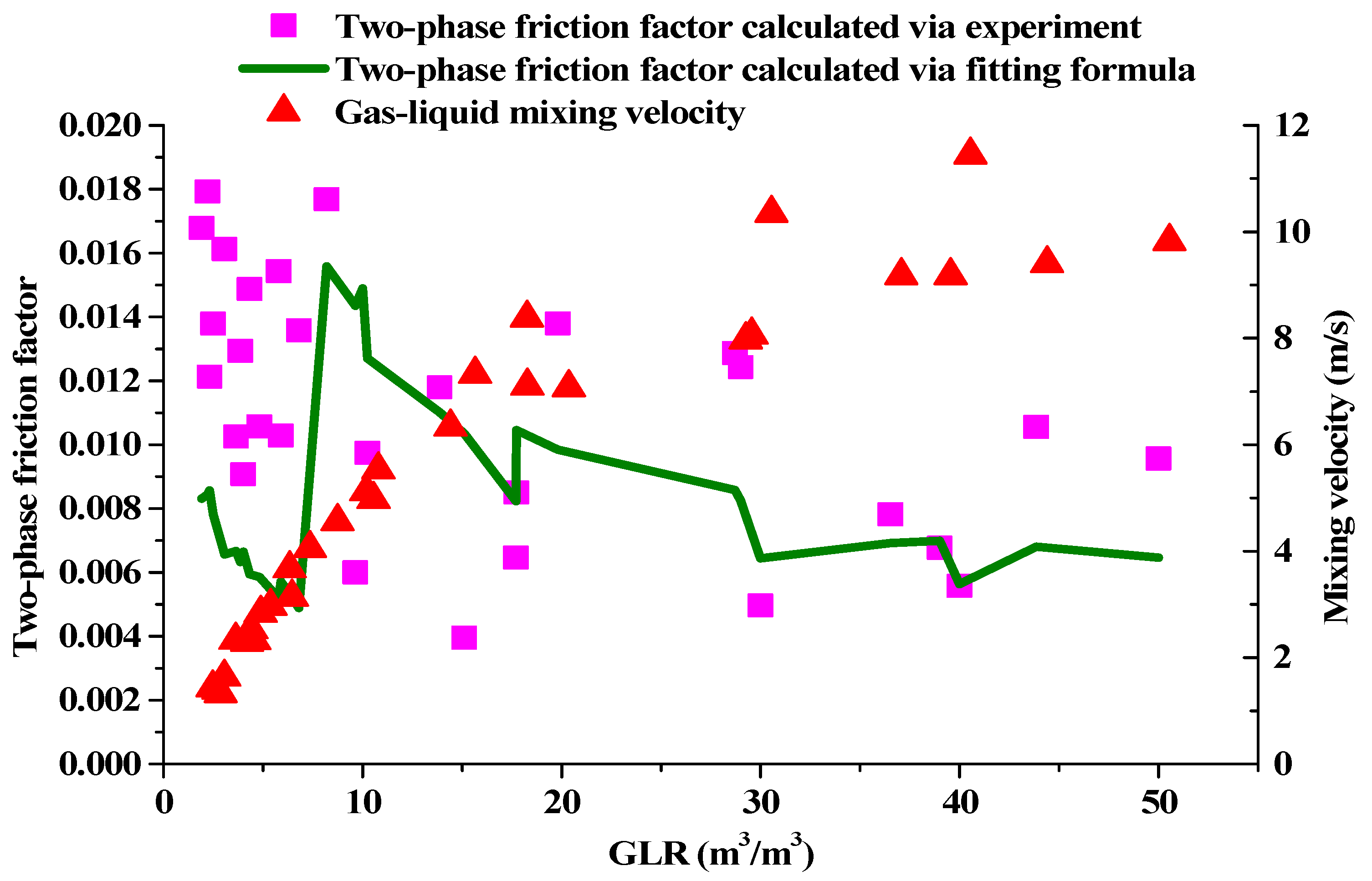
The new method is used to calculate the two-phase friction factor and pressure differential when there is axial main flow and one side hole flow. The results are presented in Figure 29 and Figure 30.
- (3)
- Analysis of the results
Uponanalyzing the experimental results of multiphase variable mass flow in a horizontal pipe, it is observed that when the gas-liquid ratio (GLR) is relatively large, the inflow from side holes has minimal impact on the pressure drop. This is because gas is compressible, and its presence does not significantly affect the pressure drop. However, when the GLR is relatively small, the pressure drop increases significantly due to side hole inflow, and the additional increase is relatively large. This substantial increase occurs because the pressure drop of a single-phase liquid flow is highly sensitive to the presence of gas. Even at low gas-liquid ratio, the gas can significantly reduce the pressure drop of the single-phase liquid flow. However, since the low gas-liquid ratio of a gas-liquid two-phase flow is similar to that of a single-phase liquid flow, the side flow can also cause a significantly increase in the pressure drop. Therefore, the side flow leads to a significant additional pressure drop.
4. Calculation and Comparison of Case Studies
4.1. Calculate Procedure
The productivity prediction method for variable mass flow published in the literature [31] is used, and the following formula is adopted for the pressure drop calculation:
in which, is the loss of mixture pressure drop obtained using the calculation method for mixture pressure drop achieved in the experiment, Pa; is unit length, m; is velocity change per unit length, 1/s; is wellbore wall shear stress, Pa; is total pressure drop loss per unit length, Pa/m.
The established model for the mixture pressure drop of single-phase variable mass flow in this study can be applied within the following ranges: main flow rate: 0.04463 to 2.6779 m/s, hole flow rate: 0.0022 to 10.1924 m/s. Verification is performed in terms of the amplitude of the impact on productivity triggered by the mixture pressure drop within this range of application.
4.2. Example 1
Take XXX-1 in Halfaya Oilfield, Iraq as an example. As shown in Table 3.
The screened wells used were 120 holes/m with a diameter of 10.0 mm, regardless of formation damage or skin factor, and the borehole roughness was taken as 0.0002 m. Assuming a single-phase flow and the reservoir of well XXX-1 is a top closed bottom water flooding reservoir and that the annular impact between the screen pipe and wellbore is ignored; then, when the FBHP is 20 MPa, the productivity prediction is made by considering and not considering the mixture pressure drop, and the calculation results are as shown in Figure 31 and Figure 32. By comparison, the following observations can be made:
- (1)
- If the mixture pressure drop is not considered, the predicted productivity results may be relatively higher. However, when compared to the total production rate, the error in production rate is close to 1% due to the limited additional pressure drop that occurs. While the increase in mixture pressure drop does reduce the production pressure differential, it is still relatively small compared to the overall production pressure differential. As a result, the effect on the total production rate of horizontal wells is only around 1%.
- (2)
- Pressure along external zone of screen pipe with considering mixture pressure drop is larger than pressure along external zone of screen pipe without considering mixture pressure drop. Flow rate along external zone of screen pipe with considering mixture pressure drop is more non-uniform than flow rate along external zone of screen pipe without considering mixture pressure drop.
The prediction result of productivity when the mixture pressure drop is not considered is as follows:
Figure 31.
Distribution of the flow rate and pressure along the outside of the screen pipe.
The prediction result for productivity considering the mixture pressure drop is as follows:
Figure 32.
The distribution of the flow rate and pressure along the outside of the screen pipe.

4.3. Example 2
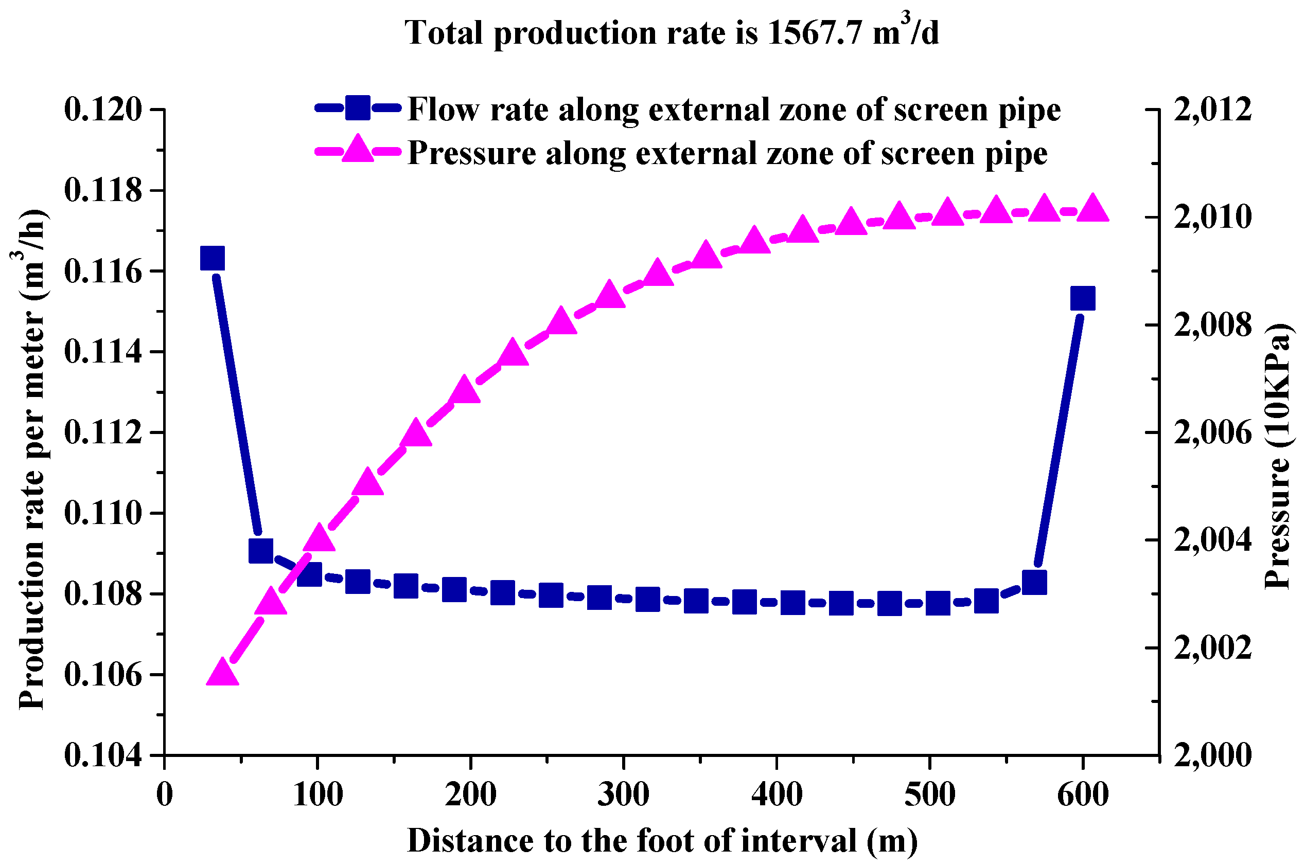
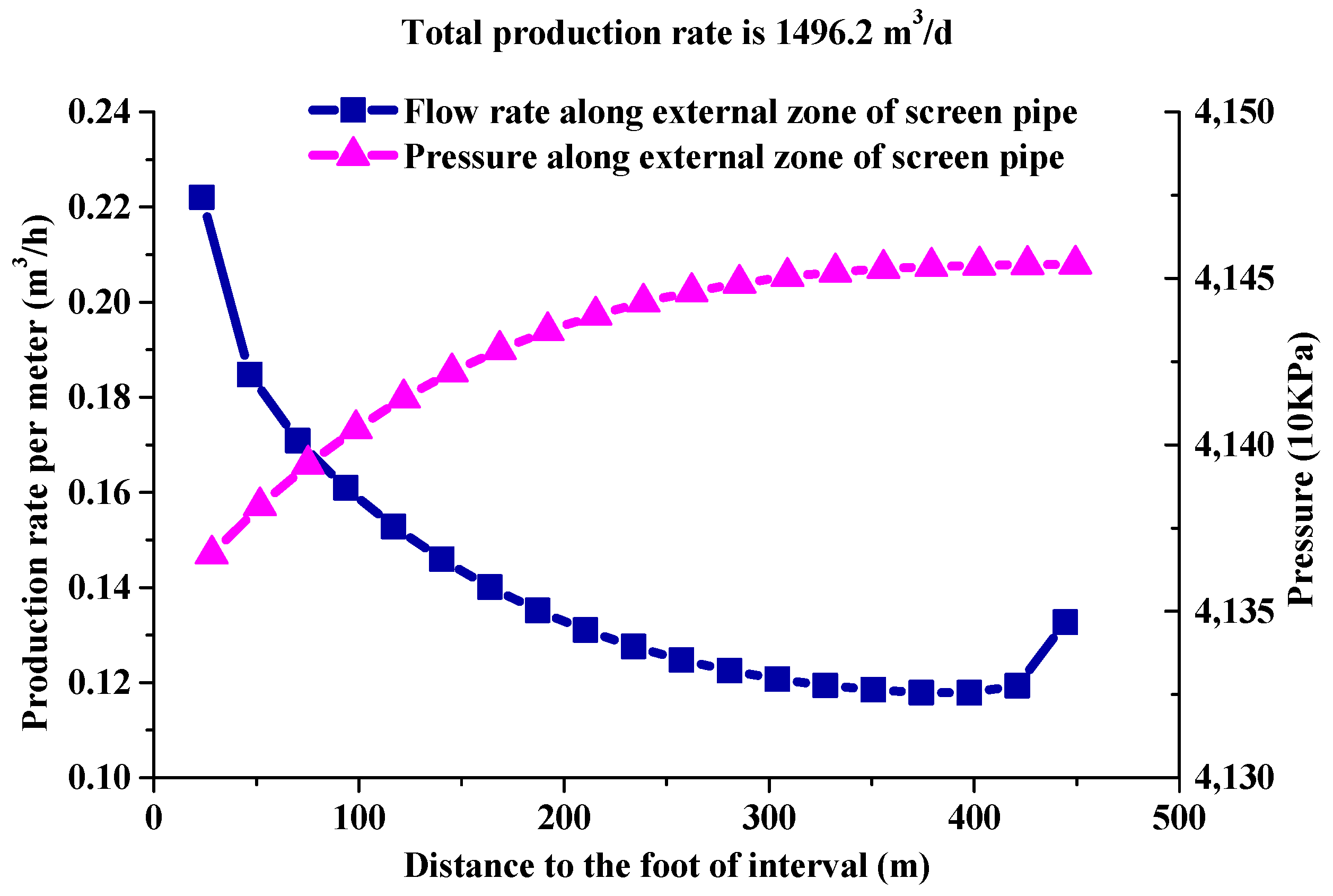
Assume the reservoir of well XXX-2 is a top closed bottom water flooding reservoir and the completion of well XXX-2 is screen completion. The Screen diameter is 0.10 m. The screened wells used were 120 holes/m with a diameter of 10.0 mm, regardless of formation damage or skin factor, and the borehole roughness was taken as 0.0002 m. Assume a single-phase flow and that the annular impact between the screen pipe and wellbore is ignored; then, when the FBHP is 41.35MPa, the productivity prediction is made by considering and not considering the mixture pressure drop, and the calculation results are as shown in Figure 33 and Figure 34. By comparison, besides the same observations as in Example 1, the production rate error of Example 2 is 52.5%. In comparison to Example 1, the mixture pressure drop and production pressure differential ratio in Example 2 are larger. As a result, the effect of the mixture pressure drop on the total production rate of horizontal wells is also larger.
The prediction result of productivity when the mixture pressure drop is not considered is as follows:
Figure 33.
Distribution of the flow rate and pressure along the outside of the screen pipe.
The prediction result for productivity considering the mixture pressure drop is as follows:
Figure 34.
The distribution of the flow rate and pressure along the outside of the screen pipe.

5. Conclusions
The following are the major findings of this study.
- (1)
- The numerical simulation for single-phase and multiphase variable mass flow in a horizontal wellbore reveals several key findings: (1) As the distance from the left inlet increases and the flow rate continues to rise, the pressure decreases, and the pressure drop becomes more pronounced in the segment with holes. This suggests that the presence of holes contributes to a significant pressure drop in the system. (2) When the total flow rate remains constant, an increase in the ratio of side injection velocity to main velocity leads to higher pressure losses and greater differences in friction factor before and after the injection hole. (3) With an increase in system pressure, the pressure drop in the wellbore also increases within the range of 0–10 m3/m3. However, in gas-liquid two-phase flow in a horizontal pipe with holes, the pressure drop initially decreases and then increases within the range of 10–20 m3/m3. This indicates a complex relationship between system pressure and pressure drop in the presence of gas-liquid two-phase flow. Overall, these simulations provide valuable insights into the behavior of variable mass flow in a horizontal wellbore and highlight the factors that influence pressure drop.
- (2)
- The study reveals that the commonly used smooth pipe friction factor, calculated as four times the Colebrook equation, does not align with the experimental data for single-phase liquid flow. Therefore, a new calculation formula for the friction factor in a horizontal pipe with holes is developed based on fitting the experimental data. This new formula provides a more accurate estimation of the friction factor in such systems.
- (3)
- The experimental results indicate that when the total flow rates are the same for the single-phase liquid flow, the friction factor with side hole flow is usually larger than the friction factor for only axial main flow, but the different friction factor proportion of the experimental results is basically the same as that of the simulation results and it is fairly small when the injection velocities ratio is small.
- (4)
- By analyzing the simulation data for single-phase variable mass flow, a linear regression equation is derived through fitting to describe the relationship between the mixture pressure drop caused by side flow and main flow velocity, as well as the ratio of side-main velocities. Comparing the fitting results obtained from this equation with the experimental data, it is observed that, for predicting the pressure drop in variable mass flow in horizontal wellbores, considering only the mixture pressure drop for the closest hole to the calculation section is sufficient, especially when the velocities of the injection holes are comparable. This finding simplifies the prediction of pressure drop in variable mass flow scenarios.
- (5)
- Upon analyzing the experimental results of multi-phase variable mass flow in a horizontal pipe, it is evident that using Dukler’s Case I method, commonly employed to predict pressure drop in conventional horizontal pipe multi-phase flow, leads to relatively small calculation results for a horizontal wellbore with holes. To address this, a new friction factor calculation method that takes slip into account is developed by referencing the Beggs and Brill method and considering two-phase friction. The new method incorporates slip and is obtained through fitting the experimental data for multi-phase variable mass flow in a horizontal pipe. By comparing and analyzing the experimental data and the fitting calculation results under different conditions, it becomes apparent that when the Gas-Liquid Ratios (GLRs) are relatively large, the presence of side flow does not significantly impact the pressure drop. However, when the GLRs are small, the side flow increases the pressure drop, and this increase is quite substantial in proportion. These findings highlight the importance of considering slip and the influence of side flow in accurately predicting pressure drop in multi-phase variable mass flow scenarios in horizontal wellbores.
- (6)
- The calculations of single-phase variable mass flow reveal that neglecting the mixture pressure drop can lead to significantly overestimated productivity prediction results, with production rate errors potentially exceeding 50%. The magnitude of the production rate error is dependent on the ratio of the mixture pressure drop to the production pressure differential. This finding, combined with the investigation of single-phase and multi-phase flows, suggests that when the Gas-Liquid Ratio (GLR) is low, the production rate error resulting from variable mass flow productivity predictions may be relatively large compared to the total production rate. Therefore, further research is necessary to develop a prediction method for the mixture pressure drop in gas and liquid two-phase variable mass flow scenarios.
- (7)
- When considering the mixture pressure drop, the pressure along the external zone of the screen pipe is higher compared to when the mixture pressure drop is not considered. Additionally, the flow rate along the external zone of the screen pipe is more non-uniform when the mixture pressure drop is taken into account, as opposed to when it is neglected. These observations highlight the impact of the mixture pressure drop on the pressure distribution and flow characteristics in the external zone of the screen pipe.
Author Contributions
Methodology, W.L.; Software, W.L.; Validation, W.L.; Investigation, W.K.; Supervision, R.L. All authors have read and agreed to the published version of the manuscript.
Funding
This article was funded by the open fund project “Study on transient flow mechanism of fluid accumulation in shale gas wells” of the Sinopec Key Laboratory of Shale Oil/Gas Exploration and Production Technology (33550000-22-ZC0613-0220).
Data Availability Statement
The raw/processed data required to reproduce these findings cannot be shared at this time as the data also forms part of an ongoing study.
Acknowledgments
Thanks to Luo Wei, the corresponding author of this article.
Conflicts of Interest
The authors declare no conflict of interest.
References
- Ihara, M.; Brill, J.P.; Shoham, O. Experimental and theoretical investigation of two-phase flow in horizontal wells. In Proceedings of the SPE 67th Annual Technical Conference and Exhibition, Washington, DC, USA, 4–7 October 1992; SPE24766. pp. 57–67. [Google Scholar]
- Ihara, M.; Shimizu, N. Effect of accelerational pressure drop in a horizontal wellbore. In Proceedings of the SPE 68th Annual Technical Conference and Exhibition, Houston, TX, USA, 3–6 October 1993; SPE26519. pp. 125–138. [Google Scholar]
- Ihara, M.; Kikuyama, K.; Hasegawa, Y.; Mizuguchi, K. Flow in horizontal wellbores with influx through porous walls. In Proceedings of the SPE 69th Annual Technical Conference and Exhibition, New Orleans, LA, USA, 25–28 September 1994; SPE28485. pp. 225–235. [Google Scholar]
- Ihara, M.; Yanai, K.; Yakao, S. Two-phase flow in horizontal wells. SPE Prod. Facil. 1995, 11, 249–255. [Google Scholar] [CrossRef]
- Su, Z.; Gudmundsson, J.S. Friction factor of perforation roughness in pipes. In Proceedings of the SPE 68th Annual Technical Conference and Exhibition, Houston, TX, USA, 3–6 October 1993; pp. 151–163, SPE 26521. [Google Scholar]
- Su, Z.; Gudmendsson, J.S. Pressure drop in perforated pipes: Experiments and analysis. In Proceedings of the SPE Asia Pacific Oil and Gas Conference, Melbourne, Australia, 7–10 November 1994; pp. 563–574, SPE28800. [Google Scholar]
- Su, Z.; Gudmundsson, J.S. Perforation inflow reduces frictional pressure loss in horizontal wellbores. J. Pet. Sci. Eng. 1998, 19, 223–232. [Google Scholar] [CrossRef]
- Plaxton, B.L. Pipeflow experiments for the analysis of pressure drop in horizontal wells. SPE Int. Stud. Pap. Contest 1995, 11, 635–650. [Google Scholar]
- Yuan, H. Investigation of single-phase liquid flow behavior in horizontal wells. In Proceedings of the Fluid Flow Projects Advisory Board Meeting, Tulsa, OK, USA, 9–10 May 1995; pp. 103–117. [Google Scholar]
- Yuan, H.; Sarica, C.; Brill, J.P. Effect of perforation density on single-phase liquid flow behavior in horizontal wells. In Proceedings of the 1996 International Conference on Horizontal Well Technology, Calgary, AB, Candada, 18–20 November 1996; pp. 603–612. [Google Scholar]
- Yuan, H.; Sarica, C.; Miska, S.; Brill, J.P. An experimental and analytical study of single-phase liquid flow in a horizontal well. J. Energy Resour. Technol. 1997, 119, 20–25. [Google Scholar] [CrossRef]
- Yuan, H.; Sarica, C.; Brill, J.P. Effect of completion geometry and phasing on single-phase liquid flow behavior in horizontal wells. SPE48937. In Proceedings of the 1998 SPE Annual Technical Conference and Exhibition, New Orleans, LA, USA, 27–30 September 1998; pp. 93–104, SPE48937. [Google Scholar]
- Ouyang, L.-B.; Arbabi, S.; Aziz, K. General wellbore flow model for horizontal, vertical, and slanted well completions. In Proceedings of the 1996 SPE Annual Technical Conference, Denver, CO, USA, 6–9 October 1996; pp. 349–361. [Google Scholar]
- Ouyang, L.-B.; Petalas, N.; Arbabi, S.; Schroeder, D.E.; Aziz, K. An Experimental Study of Single-Phase and Two-Phase Fluid Flow in Horizontal Wells. In Proceedings of the SPE Western Regional Meeting, Bakersfield, CA, USA, 10–13 May 1998. [Google Scholar]
- Ouyang, L.-B.; Aziz, K. A mechanistic model for gas-liquid flow in pipes and wells. In Proceedings of the 1999 SPE Annual Technical Conference and Exhibition, Houston, TX, USA, 3–6 October 1999; pp. 359–372, SPE 56525. [Google Scholar]
- Ouyang, L.-B.; Aziz, K. A homogeneous model for gas-liquid flow in horizontal wells. J. Pet. Sci. Eng. 2000, 27, 119–128. [Google Scholar] [CrossRef]
- Utvik, O.H.; Rinde, T.; Schulkes, R. Pressure drop in perforated pipe with radial inflow: Multiphase flow. In Proceedings of the 1997 Annual Technical Conference and Exhibition, San Antonio, TX, USA, 5–8 October 1997; pp. 1–15. [Google Scholar]
- Zhou, S.; Zhang, Q.; Li, M.; Wang, W. Experimental study on variable mass fluid flow in horizontal wellbore. J. China Pet. Univ. (Nat. Sci. Ed.) 1998, 5, 54–56+6. [Google Scholar]
- Wang, Z.; Xiao, J.; Wang, X.; Wei, J. Study on regularity of pressure drop for variable mass flow of horizotal well. Exp. Hydrodyn. 2011, 26–29, SPE38449. [Google Scholar]
- Bokane, A.; Jain, S.; Freddy, C. Evaluation and Optimization of Proppant Distribution in Multistage Fractured Horizontal Wells: A Simulation Approach. In Proceedings of the SPE/CSUR Unconventional Resources Conference—Canada, Calgary, AB, Canada, 30 September 2014. [Google Scholar] [CrossRef]
- Wang, Z.; Yang, J.; Zhang, Q.; Wang, X.; Gao, H.; Ceng, Q.; Zhao, Y. Evaluation of pressure drop prediction model for horizontal wellbore based on large size experiment. Pet. Explor. Dev. 2015, 238–241. [Google Scholar]
- Lei, H.; Chang, P.; Yang, X. Variable mass multiphase flow and fluid physical property analysis of fractured horizontal well in low—permeability tight gas reservoir. Complex Hydrocarb. Reserv. 2017, 10, 56–59. [Google Scholar]
- Wang, Z.; Zhang, Q.; Zeng, Q.; Wei, J. A Unified Model of Oil/Water Two-Phase Flow in the Horizontal Wellbore. SPE J. 2017, 22, 353–364. [Google Scholar] [CrossRef]
- Zhang, Q. Dispersed Flow Pressure Drop Model of Oil-Gas-Water Three-Phase Variable Mass Flow in Horizontal Perforated Wellbore. Liaoning Chem. Ind. 2020, 49, 443–445. [Google Scholar] [CrossRef]
- Colebrook, C.F. Turbulent Flow in Pipes, with Particular Reference to the Transition Region between the Smooth and Rough Pipe Laws. J. Inst. Civ. Eng. 1939, 11, 133–156. [Google Scholar] [CrossRef]
- Ye, Y. Numerical method of F.Colebrook formula in hydrodynamics. J. Guangdong Inst. Technol. 1986, 2, 113–115. [Google Scholar]
- Manning Francis, S.; Thompson Richard, E. Oilfield Processing of Petroleum, Vol. 1: Natural Gas; PennWell Books: Tulsa, OK, USA, 1991; p. 293. [Google Scholar]
- Asheim, H.; Kolnes, J.; Oudeman, P. A flow resistance correlation for completed wellbore. J. Pet. Sci. Eng. 1992, 8, 97–104. [Google Scholar] [CrossRef]
- Brown, K.E.; Beggs, H.D. Oil Production with Lifting Approach; Petroleum Industry Press: Beijing, China, 1987; Volume I, pp. 221–241. [Google Scholar]
- Beggs, H.D.; Brill, J.P. A Study of Two-phase Flow in Inclined Pipes. J. Pet. Tech. 1973, 25, 607–617. [Google Scholar] [CrossRef]
- Liu, X.; Guo, C.; Jiang, Z.; Liu, X.; Guo, S. The model coupling fluid flow in the reservoir with flow in the horizontal wellbore. Acta Pet. Sin. 1999, 20, 82–86. [Google Scholar]
Figure 1.
CFD model for horizontal wellbore + side hole. (a) Global map of CFD model. (b) Local region map of CFD model.
Figure 1.
CFD model for horizontal wellbore + side hole. (a) Global map of CFD model. (b) Local region map of CFD model.
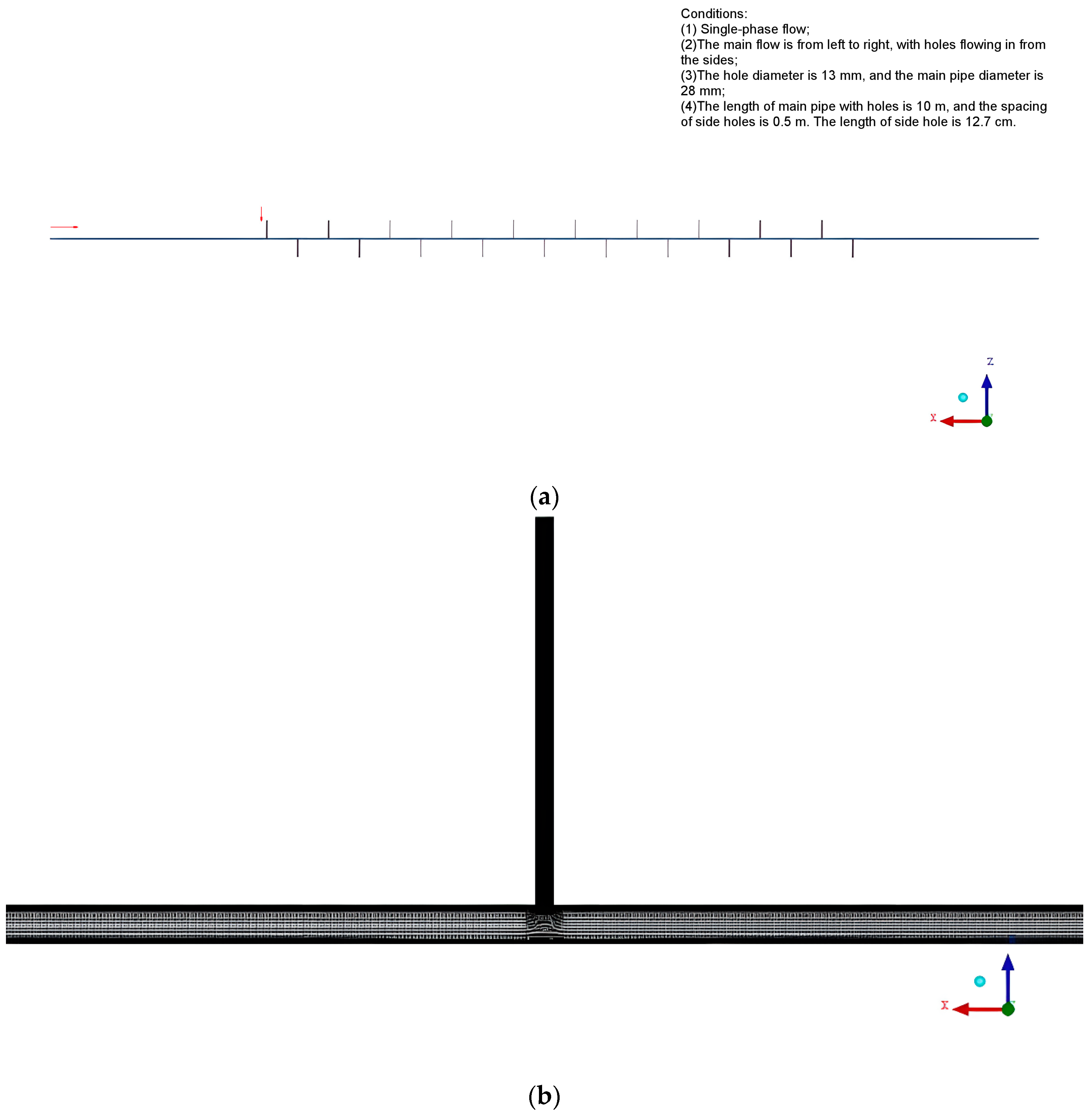
Figure 2.
Distribution of velocity field (m/s) (Taken from the leftmost part of Figure 1). (a) Global map of velocity field. (b) Local region map of velocity field.
Figure 2.
Distribution of velocity field (m/s) (Taken from the leftmost part of Figure 1). (a) Global map of velocity field. (b) Local region map of velocity field.

Figure 3.
Pressure field when there is sidestream (Pa).

Figure 4.
Variation of wellbore pressure.

Figure 5.
Pressure distribution at pipe center for single-phase liquid when the flow velocity ratio of side flow to main flow is 1.0.
Figure 5.
Pressure distribution at pipe center for single-phase liquid when the flow velocity ratio of side flow to main flow is 1.0.
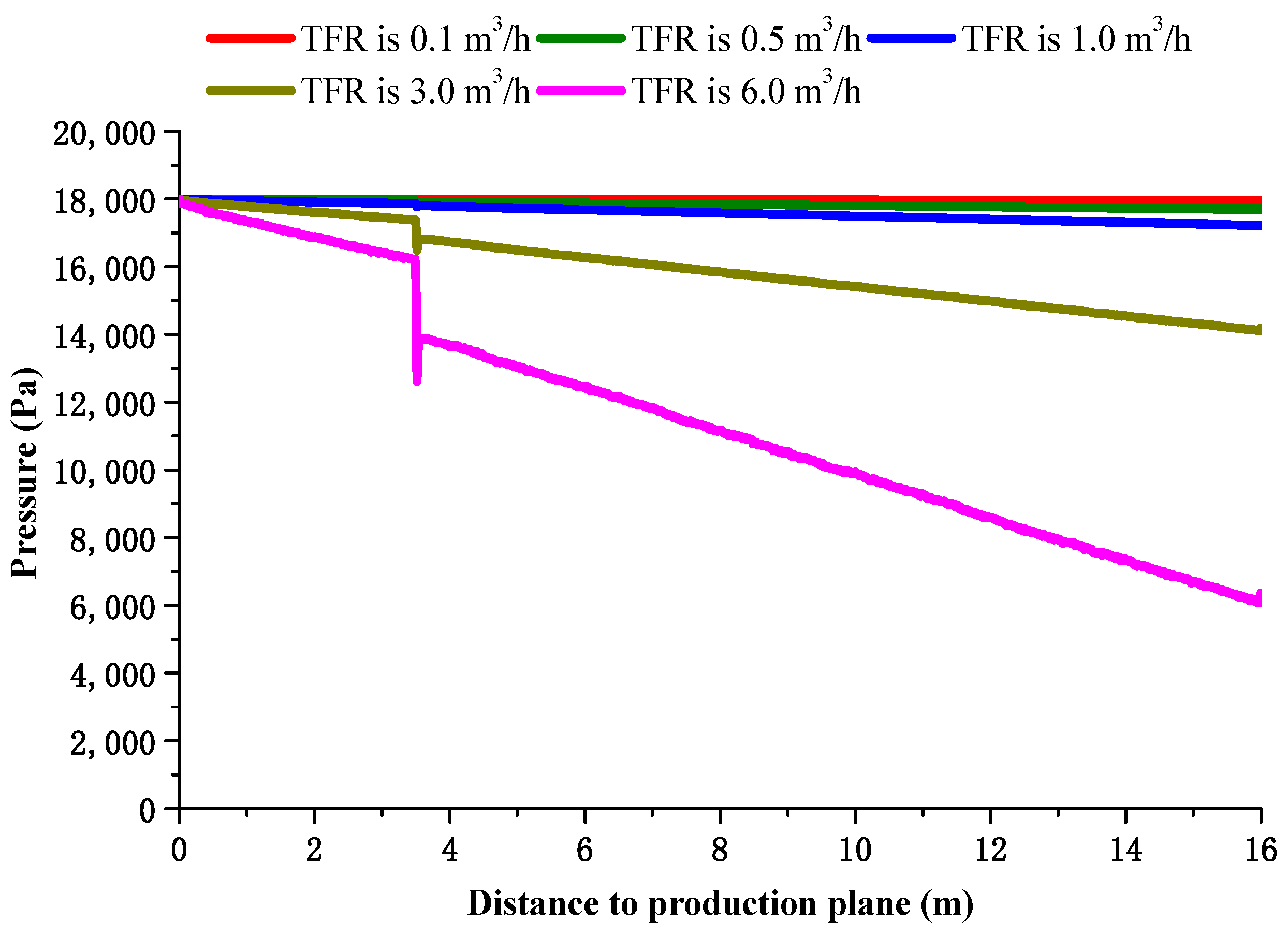
Figure 6.
Pressure distribution at pipe center for single-phase liquid when the flow velocity ratio of side flow to main flow is 5.0.
Figure 6.
Pressure distribution at pipe center for single-phase liquid when the flow velocity ratio of side flow to main flow is 5.0.
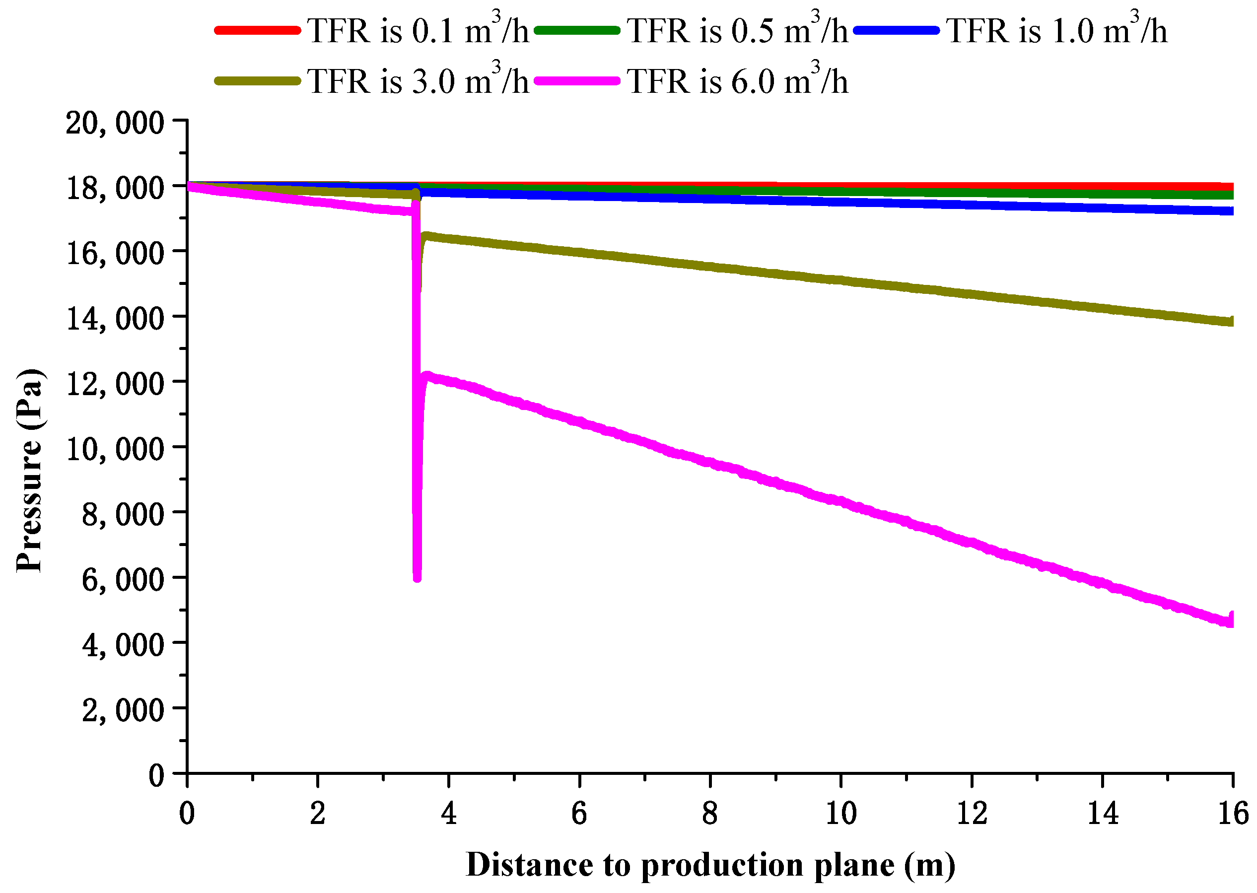
Figure 7.
Pressure distribution at pipe center for single-phase liquid when two adjacent side holes flow.
Figure 7.
Pressure distribution at pipe center for single-phase liquid when two adjacent side holes flow.

Figure 8.
Pressure distribution at pipe center for single-phase liquid when TFR is 1.0 m3/h and the flow velocity ratio of single side flow to main flow is from 0.05~20.0.
Figure 8.
Pressure distribution at pipe center for single-phase liquid when TFR is 1.0 m3/h and the flow velocity ratio of single side flow to main flow is from 0.05~20.0.
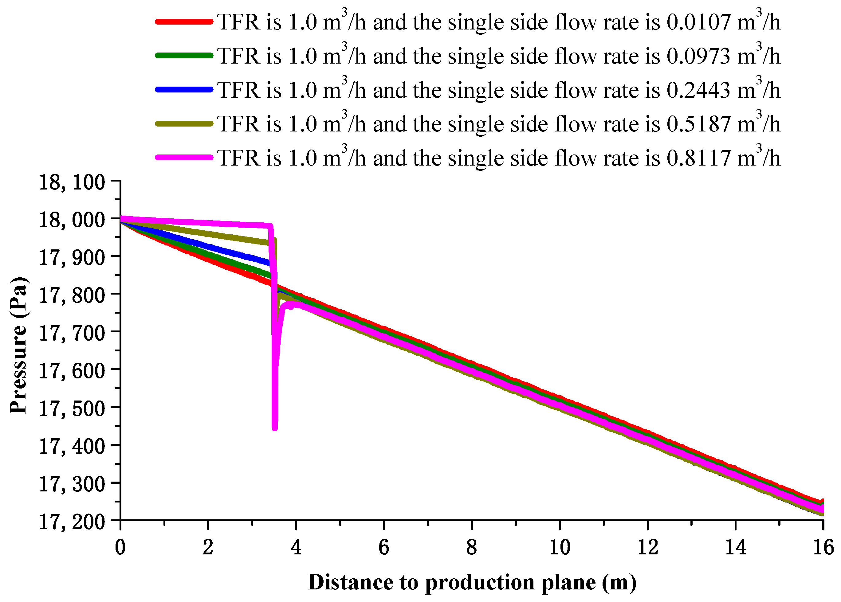
Figure 9.
The difference of friction factor before and after single injection hole at different TFR.
Figure 9.
The difference of friction factor before and after single injection hole at different TFR.
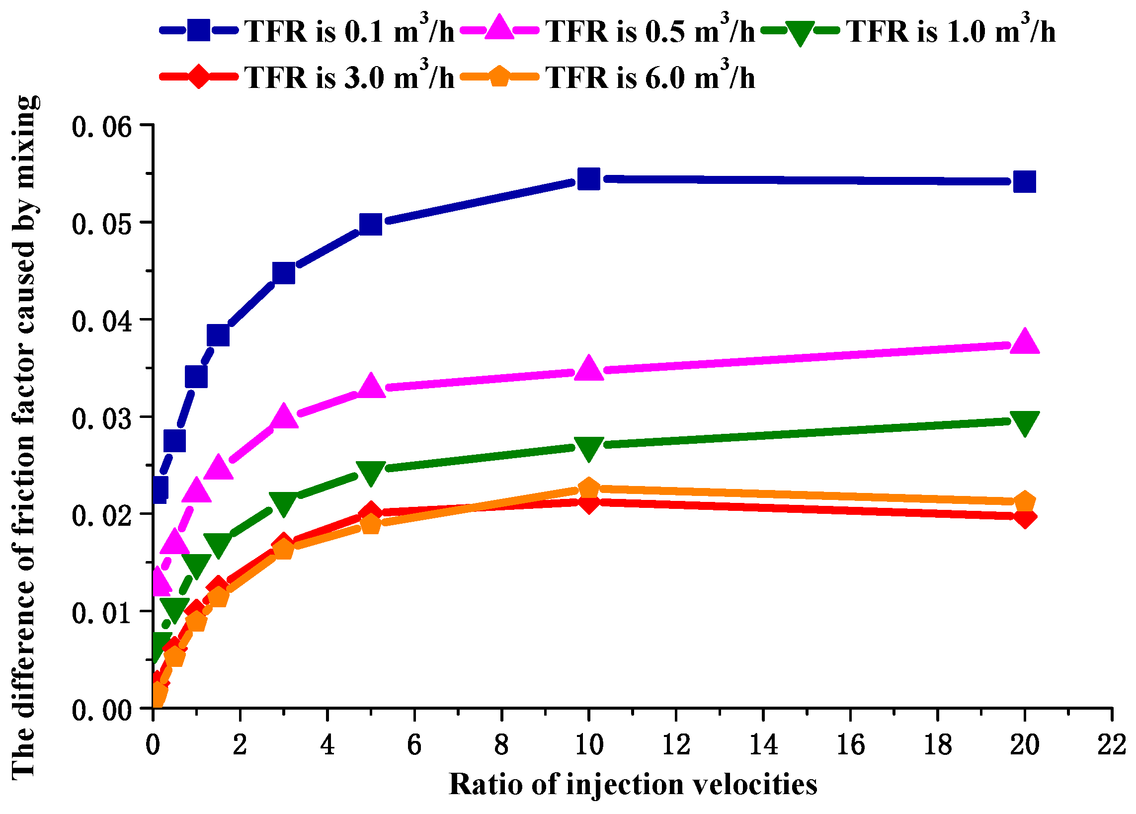
Figure 10.
Distribution of local velocity field (m/s). (a) Global map of velocity field. (b) Local region map of velocity field.
Figure 10.
Distribution of local velocity field (m/s). (a) Global map of velocity field. (b) Local region map of velocity field.
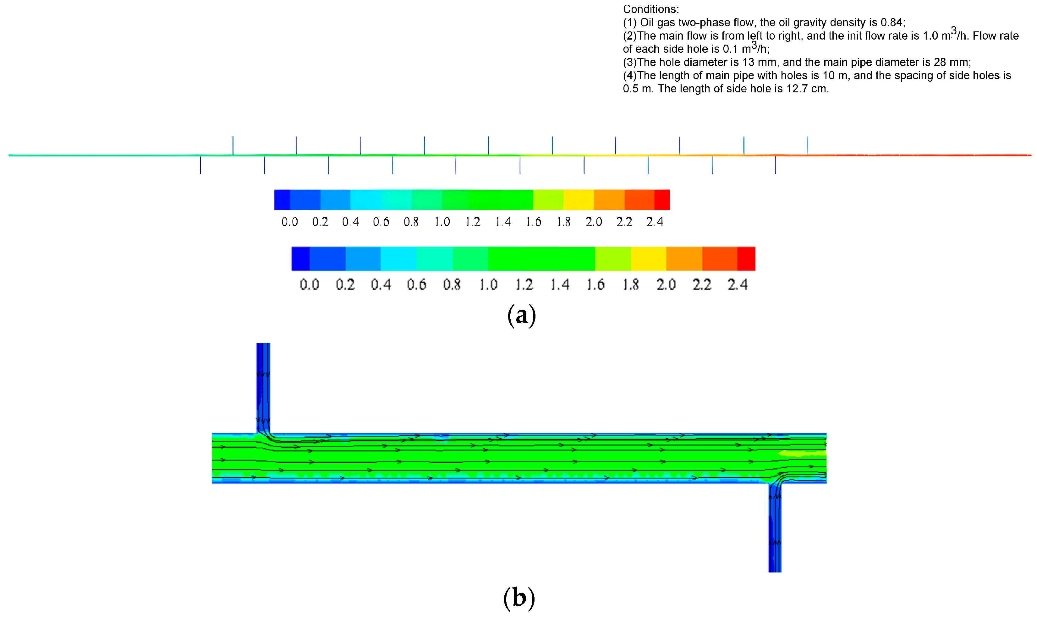
Figure 11.
Pressure field when there is sidestream (Pa).

Figure 12.
Impact on pressure distribution by GLR (system pressure 0.5 MPa).
Figure 13.
Impact on pressure distribution by GLR (system pressure 10 MPa).
Figure 14.
Impact on pressure distribution by GLR (system pressure 20 MPa).

Figure 15.
The experimental facility.
Figure 16.
Schematic of the experiment section for variable mass flow.

Figure 17.
Calculation and comparison of the experimental friction factor, fitting friction factor and four times the Colebrook friction factor.
Figure 17.
Calculation and comparison of the experimental friction factor, fitting friction factor and four times the Colebrook friction factor.

Figure 18.
Comparison of the pressure drop measured during the experiment, predicted pressure drop obtained via the fitting formula and predicted pressure drop obtained via the empirical formula (four times the Colebrook friction factor).
Figure 18.
Comparison of the pressure drop measured during the experiment, predicted pressure drop obtained via the fitting formula and predicted pressure drop obtained via the empirical formula (four times the Colebrook friction factor).

Figure 19.
Comparison of the experiment friction factor for axial main flow and single hole side flow, fitting friction factor for only axial main flow and experiment friction factor for axial main flow and two-hole side flow.
Figure 19.
Comparison of the experiment friction factor for axial main flow and single hole side flow, fitting friction factor for only axial main flow and experiment friction factor for axial main flow and two-hole side flow.
Figure 20.
Comparison of the axial main flow and single hole side flow pressure drops measured during the experiment, the pressure drop predicted for only axial main flow using the empirical fitting formula and the pressure drop of the axial main flow and two-hole side flow measured during the experiment.
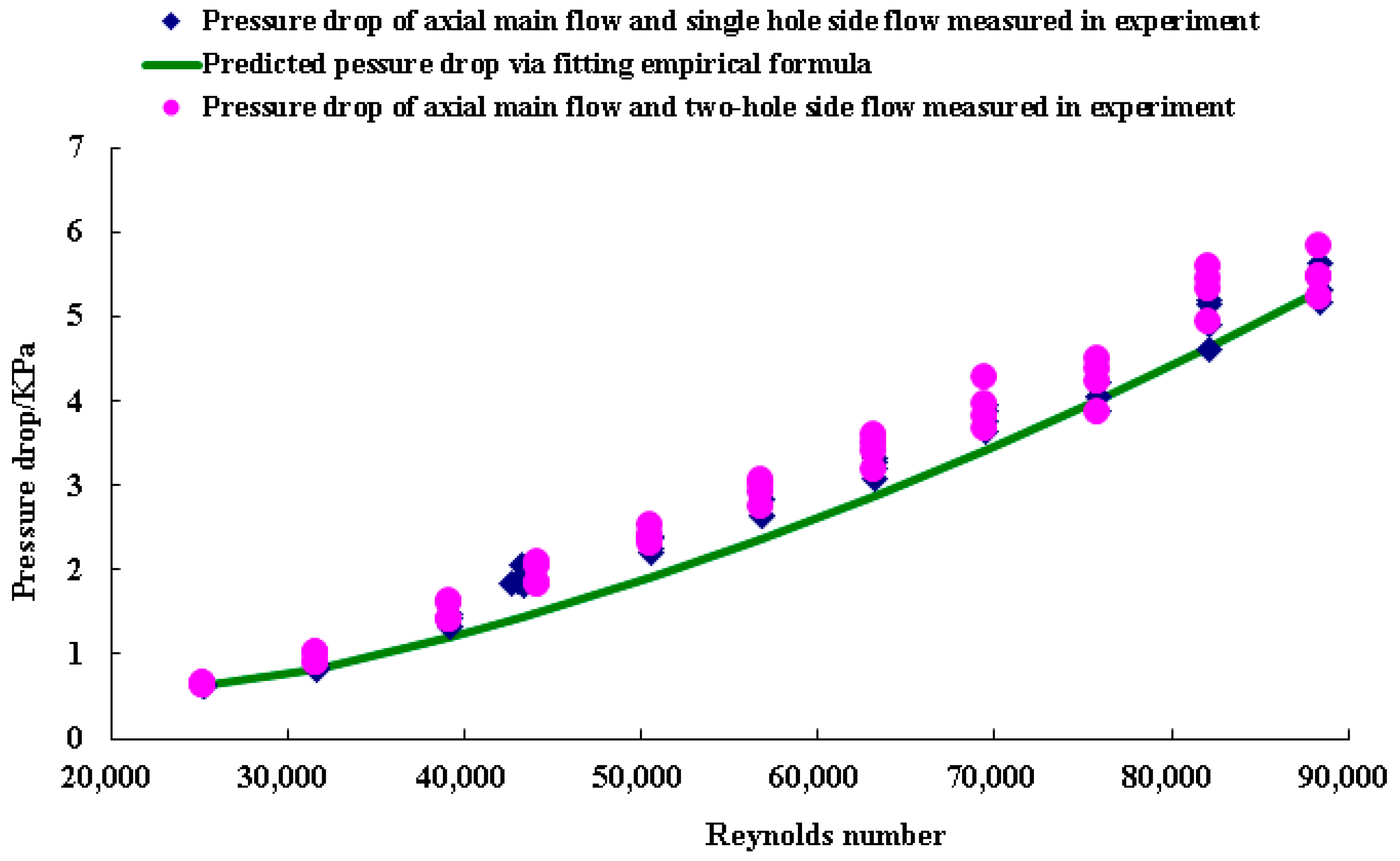
Figure 21.
The mixture pressure drop for different injection velocity ratios for the main + single side flow scenario.
Figure 21.
The mixture pressure drop for different injection velocity ratios for the main + single side flow scenario.
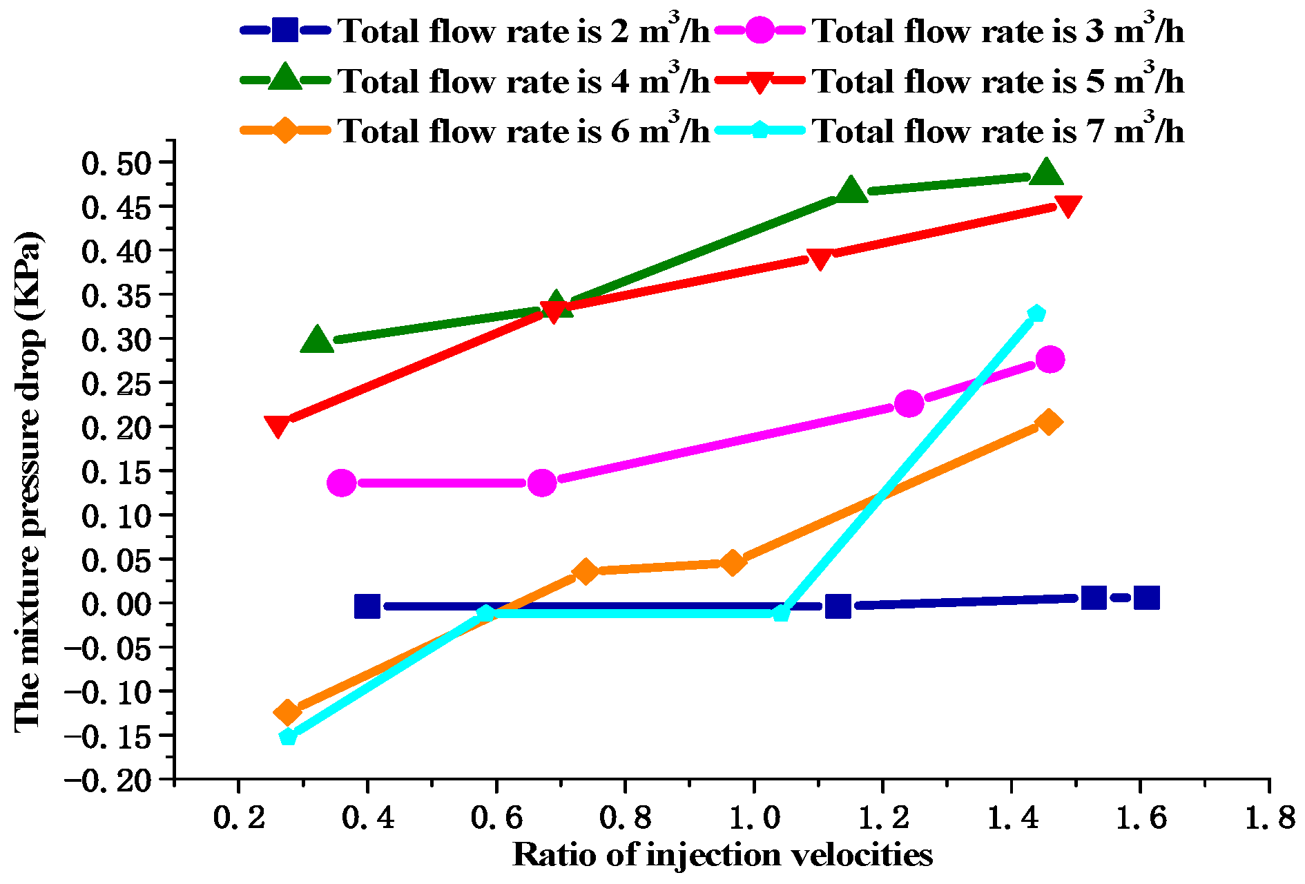
Figure 22.
The difference of the friction factor caused by mixing for different injection velocity ratios for the main + single side flow scenario.
Figure 22.
The difference of the friction factor caused by mixing for different injection velocity ratios for the main + single side flow scenario.

Figure 23.
Prediction of the pressure drop for axial and two side flows using different methods.
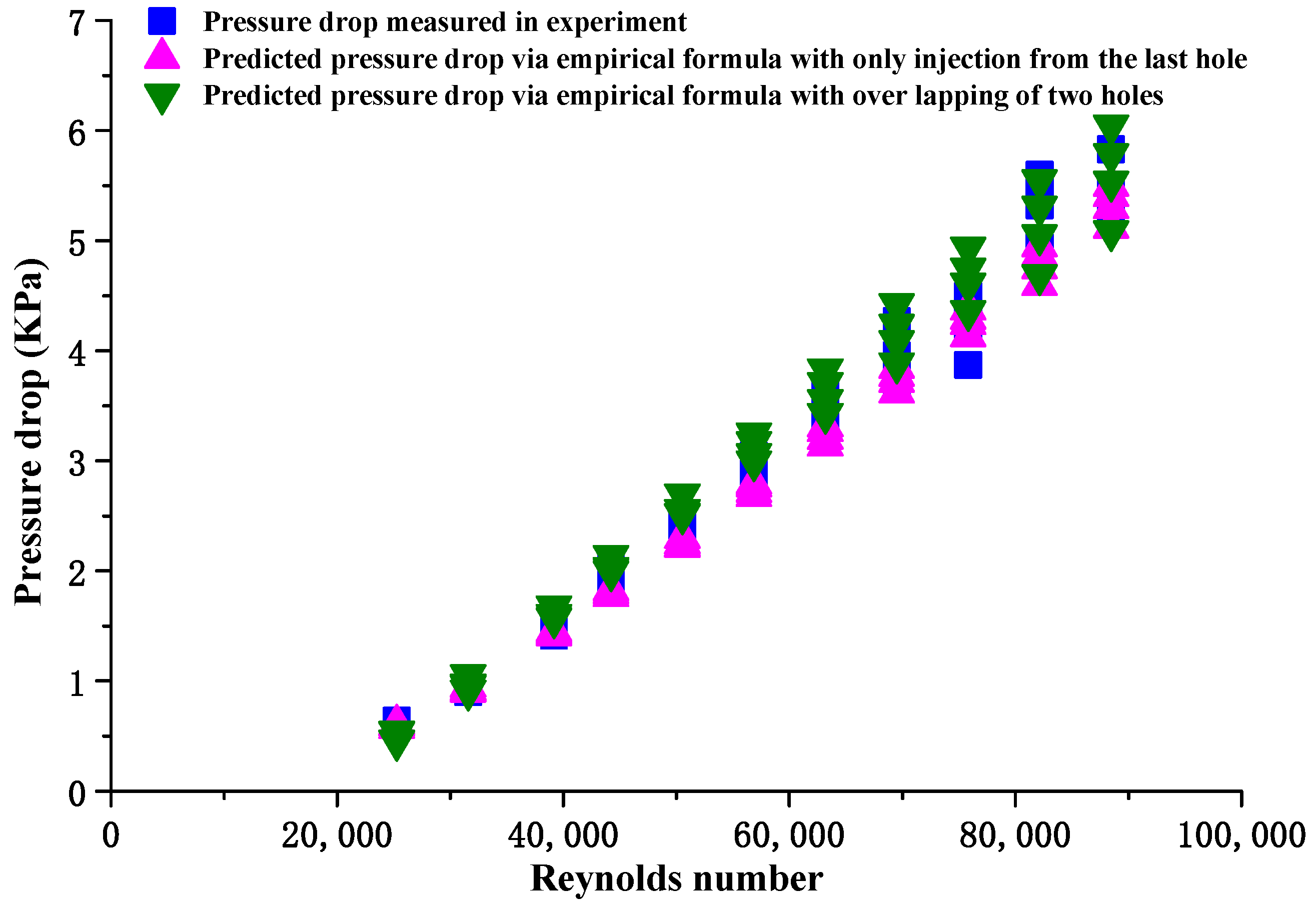
Figure 24.
Comparison of experiment pressure drop and the calculated pressure drop obtained using Dukler’s Case I method with only main flow.
Figure 24.
Comparison of experiment pressure drop and the calculated pressure drop obtained using Dukler’s Case I method with only main flow.

Figure 25.
Comparison of the two-phase friction factors achieved with only main flow in the experiment and from Dukler’s Case I method.
Figure 25.
Comparison of the two-phase friction factors achieved with only main flow in the experiment and from Dukler’s Case I method.
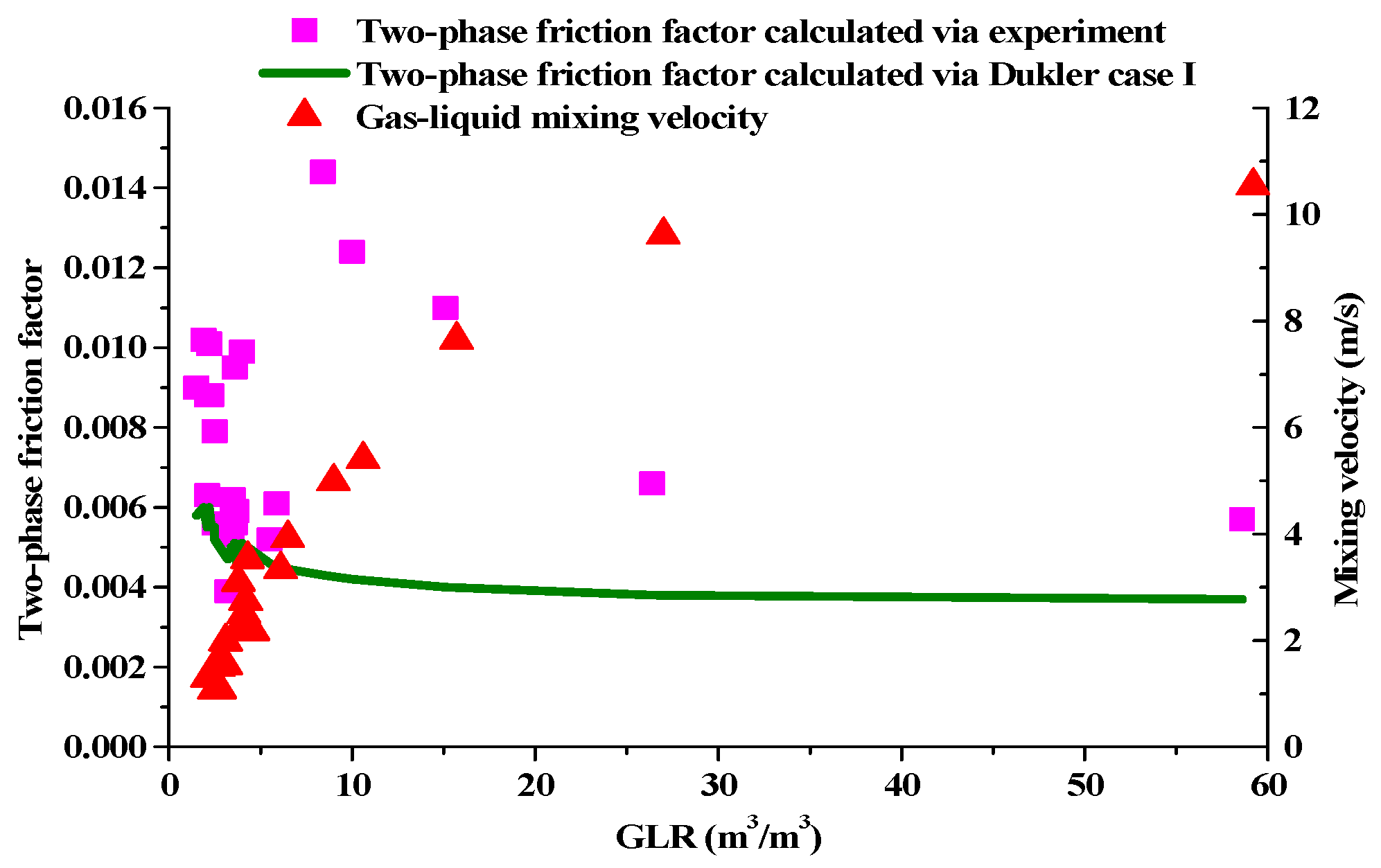
Figure 26.
Friction factors for the no-slip gas and liquid two-phase flow with variations of the two-phase flow Reynolds numbers.
Figure 26.
Friction factors for the no-slip gas and liquid two-phase flow with variations of the two-phase flow Reynolds numbers.

Figure 27.
Comparison between the pressure drop measured during the experiment (with only main flow) and the pressure drop calculated with the fitting formula.
Figure 27.
Comparison between the pressure drop measured during the experiment (with only main flow) and the pressure drop calculated with the fitting formula.
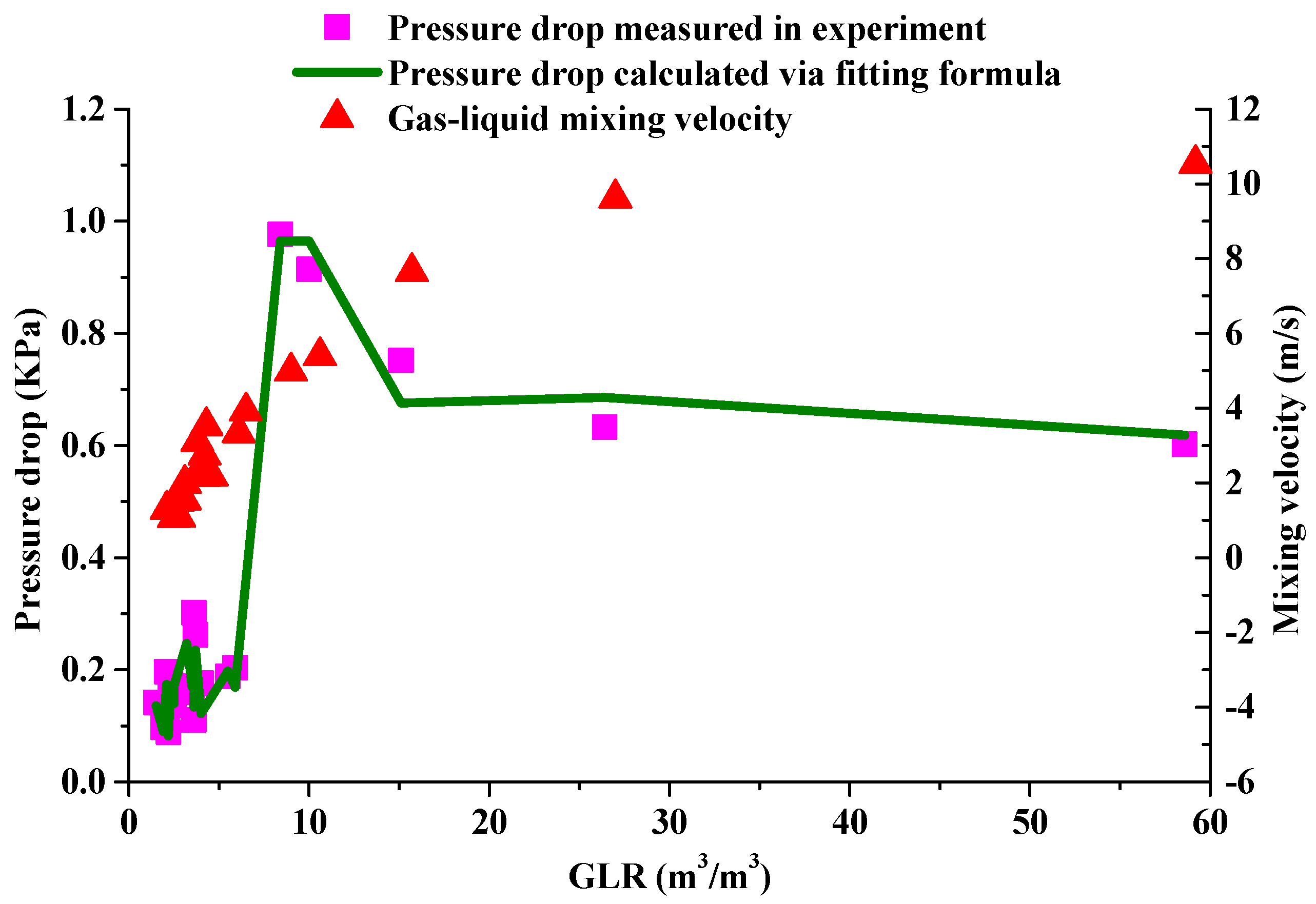
Figure 28.
Comparison between the experiment two-phase friction factor with only main flow and two-phase friction factor calculated with the fitting formula.
Figure 28.
Comparison between the experiment two-phase friction factor with only main flow and two-phase friction factor calculated with the fitting formula.
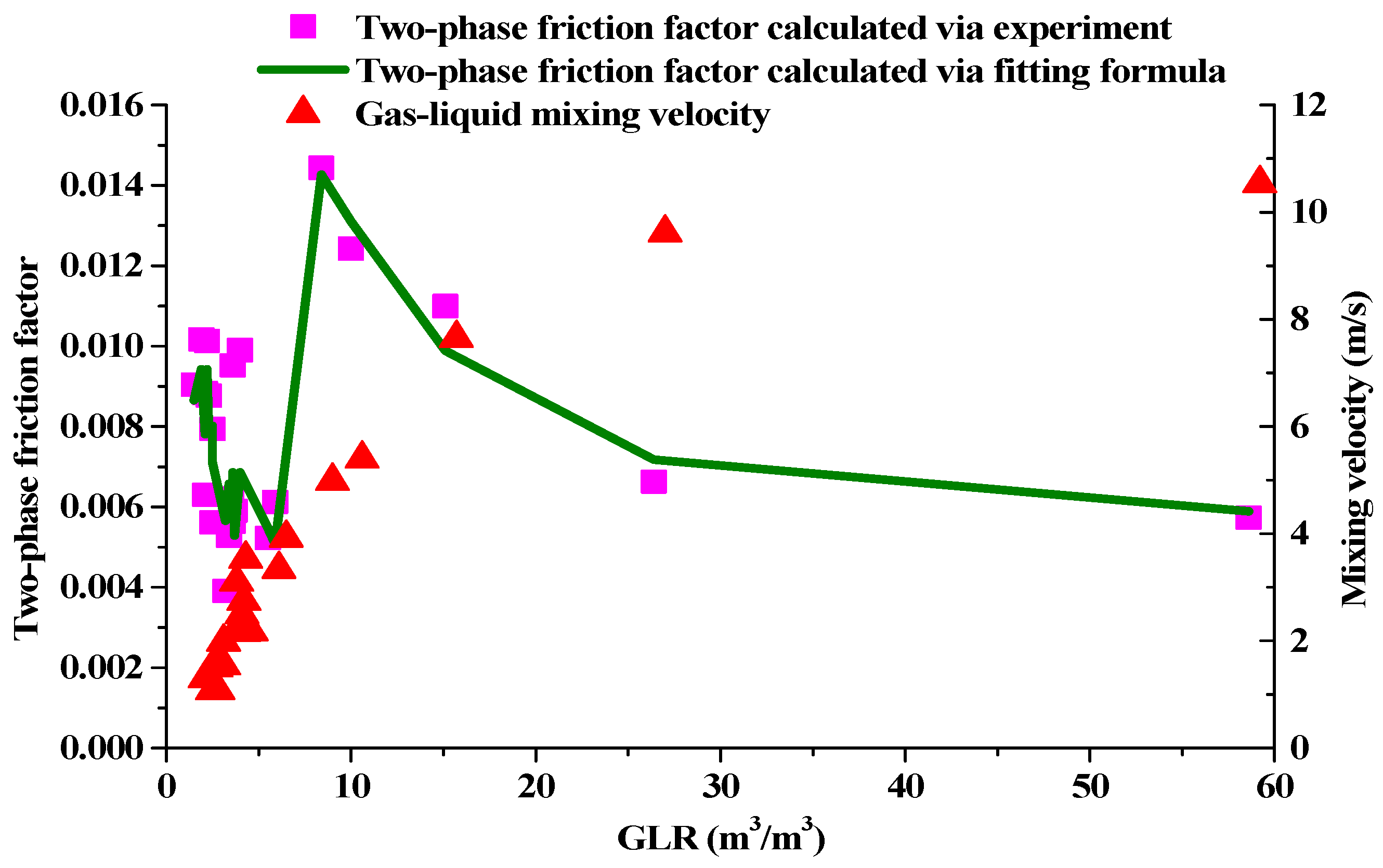
Figure 29.
Comparison of the experimental pressure drop with main and one side flow and the pressure drop calculated with the fitting formula.
Figure 29.
Comparison of the experimental pressure drop with main and one side flow and the pressure drop calculated with the fitting formula.
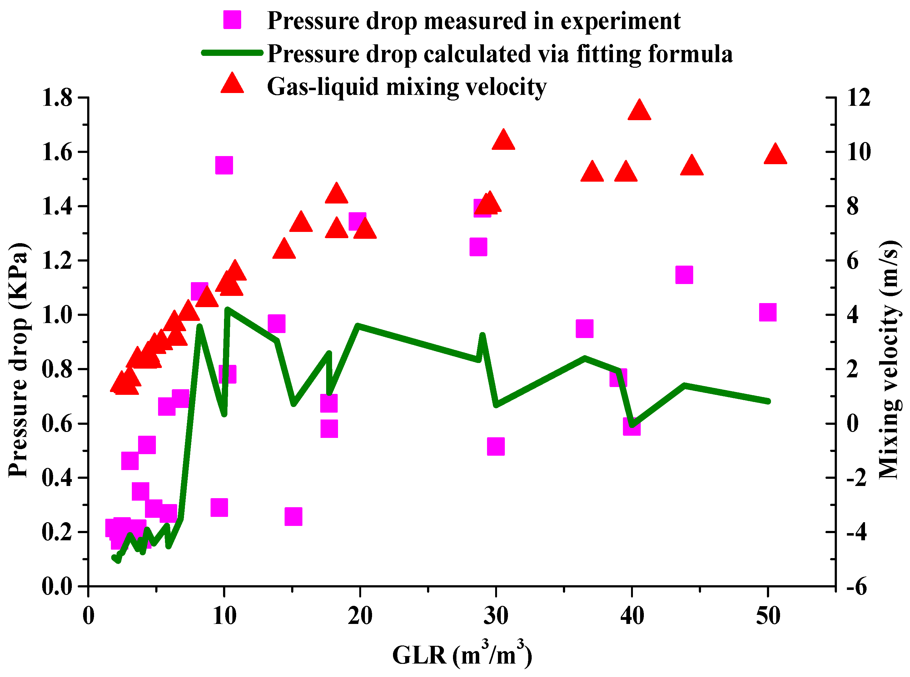
Figure 30.
Comparison of the experimental two-phase friction factor achieved with main and single side flow and the two-phase friction factor calculated with the fitting formula.
Figure 30.
Comparison of the experimental two-phase friction factor achieved with main and single side flow and the two-phase friction factor calculated with the fitting formula.

Table 1.
Device parameters.
| Equipment Type | Measurement Range | Measurement Accuracy |
|---|---|---|
| Liquid turbine flowmeter in axial pipe | 0.0~6.0 m3/h | ±0.5% |
| Differential pressure gauge | 0.0~15.0 KPa | ≤1.0 KPa |
| Gas thermal mass flowmeter in axial pipe | 0.0~10.0 m3/min | ±1.0% |
| Liquid turbine flowmeter in side pipe | 0.0~1.2 m3/h | ±0.5% |
| Gas thermal mass flowmeter in side pipe | 0.0~2.0 m3/min | ±1.0% |
Table 2.
Scope of the experiment.
| Liquid Phase Flow Rate (m3/h) | Pipe Diameter (m) | Liquid Phase Flow Velocity (m/s) | Type | Range of the Liquid Phase Flow Rate at Same Flow Velocity for 4-1/2” Screen Pipe (m3/d) |
|---|---|---|---|---|
| 1–7 | 0.028 | 0.451–3.159 | Single-phase horizontal pipe flow | 331.1–2317.7 |
| 2–7 | 0.028 | 0.903–3.159 | Single-phase variable mass flow | 662.2–2317.7 |
| 0.2–1.7 | 0.028 | 0.092–0.761 | Multi-phase variable mass flow | 68.2–558.8 |
Table 3.
Basic data from well XXX-1.
| Initial Horizontal Permeability | 13.4 | mD | Eccentric Distance | 0 | m |
| Initial vertical permeability | 1.34 | mD | Length of horizontal well | 600 | m |
| Wellbore diameter | 0.149 | m | Reservoir thickness | 30 | m |
| Crude viscosity | 1.62 | mPa.s | Crude density | 0.794 | g/cm3 |
| Crude volume factor | 1.35 | Formation pressure | 31.13 | MPa | |
| Screen diameter | 0.114 | m |
Table 4.
Basic data from well XXX-2.
| Initial Horizontal Permeability | 164 | mD | Eccentric Distance | 5.25 | m |
| Initial vertical permeability | 49.2 | mD | Length of horizontal well | 444.4 | m |
| Wellbore diameter | 0.103 | m | Reservoir thickness | 33.5 | m |
| Crude viscosity | 0.29 | mPa·s | Crude density | 0.84 | g/cm3 |
| Crude volume factor | 1.615 | Formation pressure | 41.6 | MPa | |
| Screen diameter | m |
Disclaimer/Publisher’s Note: The statements, opinions and data contained in all publications are solely those of the individual author(s) and contributor(s) and not of MDPI and/or the editor(s). MDPI and/or the editor(s) disclaim responsibility for any injury to people or property resulting from any ideas, methods, instructions or products referred to in the content. |
© 2023 by the authors. Licensee MDPI, Basel, Switzerland. This article is an open access article distributed under the terms and conditions of the Creative Commons Attribution (CC BY) license (https://creativecommons.org/licenses/by/4.0/).
Share and Cite
MDPI and ACS Style
Luo, W.; Ke, W.; Liao, R. Numerical Simulation and Experimental Investigation of Variable Mass Flow in Horizontal Wellbores: Single-Phase and Multiphase Analysis. Energies 2023, 16, 6073. https://doi.org/10.3390/en16166073
AMA Style
Luo W, Ke W, Liao R. Numerical Simulation and Experimental Investigation of Variable Mass Flow in Horizontal Wellbores: Single-Phase and Multiphase Analysis. Energies. 2023; 16(16):6073. https://doi.org/10.3390/en16166073
Chicago/Turabian StyleLuo, Wei, Wenqi Ke, and Ruiquan Liao. 2023. "Numerical Simulation and Experimental Investigation of Variable Mass Flow in Horizontal Wellbores: Single-Phase and Multiphase Analysis" Energies 16, no. 16: 6073. https://doi.org/10.3390/en16166073
Note that from the first issue of 2016, this journal uses article numbers instead of page numbers. See further details here.