Load, Electrification Adoption, and Behind-the-Meter Solar Forecasts for Alaska’s Railbelt Transmission System

Abstract

Load forecasting is an important component of power system and resource planning for electrical grids. The adoption of electric vehicles (EVs), behind-the-meter (BTM) solar, and heat pumps will significantly change the amount and variability of loads. Electrification adoption and load forecasting in arctic regions and Alaska is limited. This paper provides the first load and electrification adoption forecast for the Alaska Railbelt transmission system, including yearly adoption rates of EVs, BTM solar, and heat pumps and hourly load data for the forecasted year of 2050. The adoption rates were based on the available historical data and compared to other regional and national trends. Two forecasts were created: (1) a moderate adoption forecast based on projections from current adoption rates and comparisons to other regional and national projections and (2) an aggressive forecast, which provides an illustrative comparison of a high adoption rate of 90% for all technologies. The results of these forecasts demonstrate a significant increase in both energy, 80% and 116%, and peak load demand, 113% and 219%, for the moderate and aggressive electrification adoption scenarios, respectively. These findings highlight a need for resource planning and demand management in this region due to the adoption of EVs, BTM solar, and heat pumps.

1. Introduction

The forecasting of load and behind-the-meter (BTM) resource adoption is important for utility resource planning and balancing supply and demand. As utilities plan for grid modernization, electricity consumption must be forecast over many years. As the energy system evolves and electrifies, we see increasing electricity consumption from technologies such as heat pumps and electric vehicles, (EVs) as well as higher BTM generation from technologies such as rooftop photovoltaic (PV) solar systems. The literature is limited on the effect that cold temperatures have on BTM solar PV generation, heat pump consumption profiles, and EV charging, specifically in arctic regions. Many electrification and load forecasting studies [1] only include the contiguous US and the data on Alaska are limited. This paper provides a load and electrification adoption forecast for heat pumps, EVs, and BTM solar for 2050 for Alaska’s Railbelt electric grid.

The Railbelt is the largest regional electric grid in Alaska, spanning approximately 700 miles from Fairbanks to Homer. This Railbelt serves approximately 70% of Alaska’s population and 75% of Alaska’s electrical load [2]. Currently, approximately 80% of the Railbelt’s electricity generation comes from fossil fuels, and 20% comes from renewable sources, mainly hydro. The unique electricity landscape of the Railbelt and Alaska’s winter-peaking load contribute to many challenges to achieving the high penetration of renewables.

Decarbonization and the potential electrification of heating and transportation have significant implications for the amounts and types of new generation necessary to serve the demand. Nationwide, an all-electric approach to decarbonized space heating could require a 70% increase in electricity capacity [3]. The load forecasting studies for the US often omit Alaska and the data on Alaska are limited. It was identified that the single largest limitation to the electrification of heating is very cold temperatures in the winter that cause both a higher heating demand and lower heat pump efficiency [3]. In addition, the adoption of heat pumps may have a significant impact on the shape and time of the peak electricity demand [1]. In Alaska, despite the lower heat pump efficiencies due to cold temperatures, the high cost of heating means that heat pumps can reduce energy costs overall [4,5].

Transportation currently accounts for less than 1% of US electricity demand but accounts for 30% of primary energy consumption [1]. The adoption of EVs will increase electricity demand, including in Alaska. In 2021, there were 1250 EVs registered in Alaska [6]. The State of Alaska Electric Vehicle Infrastructure Implementation Plan predicts that in 2026, 1.01% of all registered vehicles in Alaska will be EVs, up from 0.20% EV penetration in 2021 for light-duty vehicles [6]. The cold temperatures seen in Alaska can decrease EV range by up to 50%, and colder temperatures can increase the time required to charge EV batteries [6,7]. Additionally, in cold weather, the efficiency of EVs decreases due to the energy required to keep the battery at an optimal temperature for the performance and health of the battery [7].

Forecasting solar output from BTM PV is also important for grid operators since it reduces demand on the grid. The output from solar power depends on weather conditions and can be especially variable in the winter due to snow and cloud cover. In regions such as the Railbelt that face extreme weather in winter months and very few hours of daylight, solar installations have low capacity factors (7–15%) [8]. Since the Railbelt is a winter peaking system, solar energy does not reduce the system peak demand.

Many load forecasting studies exist for the contiguous United States [9,10,11,12]. These methods use historical data, population estimates, and policy changes to estimate electrification adoption rates. Studies on forecasting load, output from BTM solar, electrification with heat pumps, and adoption and charging profiles of EVs are understudied for the arctic regions, including Alaska. The load forecasts that were performed have not included load changes due to the adoption of electrification technologies such as heat pumps and electric vehicles and BTM solar [13,14]. The contribution of this paper is that it provides the first Railbelt region wide load and electrification adoption forecast for the Alaska Railbelt transmission system. The load forecasts produced include yearly adoption rates for EVs, BTM solar, and heat pumps and the hourly load demand for the year 2050.

This paper is organized into the following sections: Section 2 provides general information relevant to the forecasts. Section 3 provides the methods, data, and resulting yearly forecasts for the adoption of EVs, heat pumps, and BTM solar. Section 4 provides the methods, data, and resulting hourly load data for EVs, heat pumps, BTM solar, and the total load. Section 6 concludes with a summary of the key findings and implications of the forecasts.

2. Electrification and BTM Solar Baseline Information

This section outlines the data and methods used to estimate the baseline information necessary to create the electrification adoption forecasts. These data include a population forecast, the number of buildings, and the number of vehicles.

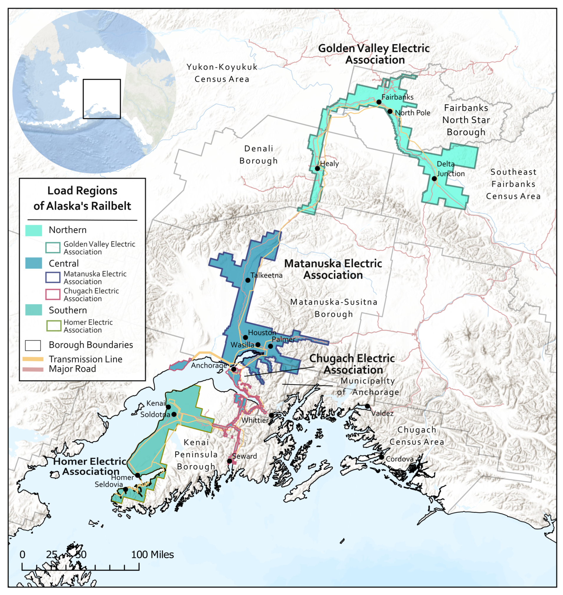
The collected data were categorized by electric utility and general load area. There are four electric cooperatives in the Railbelt: Golden Valley Electric Association, Matanuska Electric Association, Chugach Electric Association, and Homer Electric Association. There are three general load areas in the Railbelt, which are connected vertically with a single transmission line: Northern, Central, and Southern. These boroughs, utility service areas, and load areas are illustrated in Figure 1.

2.1. Population

Alaska’s population has declined from 742,874 in 2015 to 734,323 in 2020 [15]. It is forecasted that Alaska’s population will increase from 2021 to 2040, then in 2040 the rate of change becomes relatively stable until 2050, as illustrated in Figure 2 [15].

The forecasted population growth from 2023 to 2050 is approximately 3%. Due to the negligible forecasted population change in Alaska, it is estimated that the number of buildings and vehicles will also remain constant through 2050.

2.2. Number of Buildings

The number of buildings receiving electricity from the Railbelt transmission system was calculated using property information from the Fairbanks NorthStar Borough (FNSB), Kenai Peninsula Borough (KPB), Matanuska-Sustina Borough (MSB), and the Municipality of Anchorage (MOA).

The property information collected from the boroughs and the Municipality of Anchorage included address, year built, and primary use of property. This information was used to determine the number of residential, commercial, and non-residential or non-commercial buildings in these boroughs and the municipality. Industrial buildings were not evaluated as part of this study.

The Denali Borough, the City of Nenana, and the City of Delta are also located along the Railbelt; however, no property information is available for these locations. The Denali Borough includes the towns or cities of Anderson, Healy, Cantwell, and Denali Park. In the absence of property information from these locations, census data from the 2018 American Community Survey for Physical Housing Characteristics for Occupied Housing Units [16] were used. The number of occupied housing units from the census data was used as the number of residential buildings for these locations. The number of commercial buildings was estimated by using the ratio of residential to commercial buildings from FNSB for the locations with more commercial activity, such as Denali Park, and MSB for the locations with less commercial activity, such as Nenana, Delta Junction, Anderson, Cantwell, and Healy.

The number of commercial and residential buildings receiving electricity from the Railbelt transmission system are outlined in

Table 1. Building Counts for the Railbelt. * estimate based on census.

Area	Electric Utility	Load Region	Residential	Commercial	Total
Fairbanks North Star Borough	GVEA	Northern	29,100	14,992	44,092
Healy *	GVEA	Northern	377	25	402
Cantwell *	GVEA	Northern	93	6	99
Denali Park *	GVEA	Northern	44	23	67
Anderson	GVEA	Northern	50	3	53
City of Nenana *	GVEA	Northern	159	10	169
City of Delta Junction *	GVEA	Northern	320	21	341
Matanuska-Susitna Borough	MEA	Central	51,145	3,375	54,520
Municipality of Anchorage	CEA	Central	87,618	10,964	98,582
Kenai Peninsula Borough	HEA	Southern	43,937	4550	48,487

.

The total number of buildings by load region are:

• Northern: 45,223
• Central: 153,102
• Southern: 48,487
• Total: 292,035

2.3. Number of Vehicles

The number of vehicles was determined by the number of registered vehicles in 2022, as listed by the Department of Motor Vehicles (DMV) for FNSB, Delta Junction, MSB, KPB, City of Delta Junction, City of Nenana, and MOA [17]. The types of vehicles for which DMV reports data include passenger, motorcycle, commercial trailer, trailer, commercial truck, pickup, bus, and snowmobile. This study considered the electrification of the following vehicle types: car (DMV “passenger” type), truck (DMV “pickup” type), box truck (DMV “commercial truck” type), and bus. The number of vehicles by type and by area are outlined in

Table 2. Vehicle Counts for the Railbelt.

Area	Electric Utility	Load Region	Car	Truck	Box Truck	Bus	Total
Fairbanks North Star Borough	GVEA	Northern	54,009	27,107	7393	385	88,894
City of Nenana	GVEA	Northern	343	231	43	2	619
City of Delta Junction	GVEA	Northern	2632	1728	332	29	4721
Matanuska-Susitna Borough	MEA	Central	47,483	24,556	4048	513	76,600
Municipality of Anchorage	CEA	Central	186,739	64,251	16,620	871	268,481
Kenai Peninsula Borough	HEA	Southern	33,432	21,998	3895	223	59,548

.

The total vehicles by load region are:

• Northern: 94,234
• Central: 345,081
• Southern: 59,548
• Total: 498,863

3. Yearly Forecasts

The forecasts generated as a part of this study included projections for EVs, BTM PV, heat pumps, and the existing load base. The local and global trends, along with population estimates and policy changes were used to project growth rates as a method to generate an estimate of the load growth and electrification adoption through 2050.

Two load forecasts were generated to represent two trajectories for the adoption of electrification and residential solar generation. These forecasts are called the moderate and aggressive forecasts. The moderate forecast was determined by following the current adoption of technologies and forecasts generated by other Alaskan entities. The aggressive forecast was set to assume 90% of buildings (residential and commercial) would adopt heat pumps and residential solar, and 90% of vehicles would be electric vehicles in 2050. Therefore, the aggressive forecast provides a comparison of the current trends with a near total adoption of these technologies to illustrate the impacts to the load. The aggressive scenario is provided as an illustrative comparison and not as a realistic scenario. The inputs, assumptions, and methods used to generate these forecasts are outlined below, along with the resulting projections.

3.1. Electric Vehicles

3.1.1. Methods

The Alaska Energy Authority (AEA) produced two EV growth forecasts through 2026, continued and aggressive, for the state of Alaska as part of their Electrical Vehicle Infrastructure Implementation Plan [6]. The forecasts were scaled from all of Alaska to just the Railbelt by assuming 76% of vehicles in the AEA Alaska forecasts were on the Railbelt, which was based on the number of registered vehicles in the state versus in the communities along the Railbelt. The historical growth rates for electric vehicles in Anchorage were obtained from CEA’s electric vehicle information [18]. The AEA forecasts and the historical numbers of EVs on the Railbelt can be seen in Figure 3.

The AEA forecasts were then extended to 2050 following 2nd degree polynomial growth, which follows historical growth. The moderate forecast of EV adoption in this study was assumed to be the result of the extended AEA aggressive forecast.

3.1.2. Results

In 2050, the number of EVs on the Railbelt for the moderate forecast was projected to be 353,381, which equates to 71% of vehicles based on the 2022 Alaska DMV number of registered vehicles in the Railbelt. The aggressive forecast for this study assumes 90% of vehicles will be EVs, which equates to 449,000 vehicles. These forecasts are illustrated in Figure 4.

These EV adoption forecasts were compared to other regional, national, and global forecasts in terms of a percentage of vehicles. These other forecasts included the Bloomberg Electric Vehicle Outlook for Electric Vehicles [19] for leading markets, as the United States is considered a leading market; ISO-NE EV forecasts [20], as a comparison to another cold region in the United States; and national EV adoption forecasts from [21]. These comparisons are illustrated in Figure 5.

The Railbelt EV adoption forecast is slightly lower than ISO-NE, the United States, and global leading market adoption forecasts, as seen in Figure 5. The Railbelt adoption rate in 2030 is approximately 10%, compared to 15–25% adoption for the other regions. This lower adoption rate is reasonable and is expected for the Railbelt in Alaska due to the increased energy use both while parked and while driving in a cold climate, as outlined in [22].

3.2. Behind-the-Meter Solar

3.2.1. Methods

The primary constraints for solar PV adoption in Alaska include the lack of state incentives such as a renewable portfolio standard (RPS). The BTM solar incentives available to Alaska include the federal investment tax credit (ITC) and local solarize programs where discounts are available for community-wide solar installations. The ITC provides a 30% discount for solar PV installation between 2022 and 2032, decreasing to 26% in 2033, and 22% in 2034 [23]. Despite the lack of state incentives or mandates for renewable energy generation, the Railbelt has experienced the exponential growth of BTM capacity for solar PV, illustrated in Figure 6 [24].

The BTM solar forecast generated in this work used several factors to determine growth rates, including:

• ITC expiration date,
• Projected electricity prices,
• Projected solar costs.

The Energy Information Administration’s (EIA) energy outlook predicts the national electricity rates to increase linearly beginning around 2027 [25]. The National Renewable Energy Laboratory’s (NREL) annual technology baseline (ATB) for residential and commercial PV costs (levelized cost of energy (LCOE), operations and maintenance (O&M), capital expenditures (CAPEX)) shows decreasing costs for both the moderate and advanced scenarios until 2030 then decreases at a lower rate after 2030 [26]. These electricity and solar cost forecasts are illustrated in Figure 7.

The historical Railbelt BTM solar capacity was compared to other BTM solar forecasts across the United States, including the states within ISO-NE’s territory (Maine, Massachusetts, Vermont, New Hampshire, Connecticut, and Rhode Island) [9], representing a cold region, and Hawai’i [27], representing a region with very high BTM solar installation rates. The Hawai’i installed capacity is from the Hawaiian Electric, Hawai’i Electric Light, and Maui Electric covering the islands of Maui, Lana‘i, and Moloka‘i. For equal comparison between regions, the installed capacity forecasts were normalized by the 2013 amount of the installed BTM solar capacity. These comparisons are shown in Figure 8.

For perspective, the historical BTM solar installed capacity as a percentage of the peak load was 0.5% in ISO-NE (2022 net peak load in ISO-NE was 24,780 MW [28]), 74.7% in Hawai’i (2020 net peak load in HECO was 1,496 MW: Hawai’i was 183 MW [29], O‘ahu was 1116 MW [30], Moloka‘i was 5.8 MW, Lana‘i was 6.14 MW, Maui was 185.3 MW [31]), and 1.5% in the Railbelt (2021 net peak load in Railbelt was 765.3 MW). Note that Hawai’i and ISO-NE are summer peaking systems, and therefore, BTM solar will impact the peak load in those regions. In the Railbelt, the peak load occurs in winter, and therefore, BTM solar will have the most impact during the lowest load period in the summer, which was 381 MW in 2021. Therefore, the 2021 Railbelt BTM solar capacity as a percentage of the minimum summer load is 4.8%. ISO-NE and Hawai’i will have a greater amount of energy generation per installed capacity due to high capacity factors in those regions with lower latitudes compared to the Railbelt. Therefore, even though the percentage of BTM solar by installed capacity to peak load and minimum load is larger in the Railbelt compared to ISO-NE, ISO-NE experiences a greater impact from BTM solar in terms of total energy generation.

A significant finding is that the Railbelt in Alaska is experiencing a similar growth rate (not total amount) in BTM solar to ISO-NE, compared to peak load and as normalized by the 2013 installed capacity. This growth rate is similar despite lower capacity factors in the Railbelt and a lack of state incentives for BTM solar in Alaska. The growth rate as normalized by the 2013 installed capacity in Hawai’i is lower compared to ISO-NE and the Railbelt. Hawai’i’s lower growth rate is likely due to reaching hosting capacity limits of the distribution and transmission systems in Hawai’i due to the high percentage as compared to the peak load (74.7%). Therefore, it is reasonable to expect continued BTM solar growth rates in the Railbelt similar to those that are currently seen.

3.2.2. Results

For the moderate electrification forecast, this work estimates a series of decreasing growth rates to reflect impacts from the ITC and solar installation costs. From 2023 through 2027, this work predicts continued exponential growth in BTM solar, based on the historical exponential growth shown in Figure 6. This exponential growth is estimated to continue until 2027, halfway through the duration of the ITC.

From 2025 through 2027, it is estimated that solar installations will continue to increase linearly due to the ITC and continued projected solar installation cost reductions. The linear growth rate is based on the rate of change from 2025 to 2027, which equates to approximately 3318 customers per year. This rate of change was applied from 2028 to 2033, a year after the 30% ITC discount ends, to reflect possible construction delays.

From 2034 to 2040, the estimated solar installation costs reduce at a lower rate, and the ITC discount decreases to 26% and 22% for systems installed by 2033 and 2034, respectively. Therefore, for this time period, it was estimated that BTM solar adoption would continue to increase but at half of the previous rate, at 1659 customers per year.

Over time, the percentage of households that can afford to install solar PV that have not already done so will decrease. This is expected to have a negative impact on solar adoption in the absence of solar incentive programs for low- and middle-income households. Therefore, for the period from 2040 through 2050 the growth rate was estimated to halve again, to 829 customers per year to reflect this impact. By the end of 2050, the projected number BTM solar installations was 53,386. Given that the number of residential and commercial buildings in the Railbelt is 292,035, this is equivalent to 18% of residential and commercial buildings in the Railbelt with BTM solar installations.

The total installed BTM solar capacity was calculated using the current typical BTM solar installation size of 5 kW per installation. The BTM solar forecast by number of installations and by capacity is shown in Figure 9. For comparison, the Solar Energy Industries Association’s (SEIA) five year growth projection for Alaska was also included in Figure 9 at a total of 69 MW in 2027, which closely matches the proposed moderate BTM solar forecast.

The aggressive solar forecast assumes 90% of residential and commercial buildings having BTM solar by 2050. This equates to 262,832 houses and a total installed capacity of 1314 MW based on a 5 kW typical installation size.

3.3. Heat Pumps

3.3.1. Methods

The heat pump adoption rate assumes a new installation of a heat pump and does not assume the full replacement of the heating systems. Most of the Railbelt has temperatures that routinely fall below the efficient operating range of heat pumps, making a back up heat source necessary. The purpose of this heat pump adoption forecast is to estimate the impact of heat pump installations on load and not to transition all heating sources to electricity.

The CEA generated a heat pump forecast for the CEA service territory [32]. This heat pump forecast was expanded to include all of the Railbelt and extrapolated to 2050. The CEA moderate and aggressive forecasts were continued at the same growth rate from the original forecast of 2032 out to the target of 2050 for this study. The forecast was also increased by 97% to expand to the entire Railbelt based on the number of buildings in the CEA versus the entire Railbelt. The forecasts are shown in terms of number of installations and by the installed capacity, assuming a 3.2 kW rating per heat pump in Figure 10.

The ISO-NE’s 2022 Heating Electrification Forecast was used to provide comparison to the Railbelt heat pump forecasts. The forecasts were normalized by the number of installations in 2022 to provide a comparison of the forecasted growth rates. These normalized heat pump growth forecasts are shown in Figure 11.

The heat pump forecasts for 2023 from ISO-NE and from CEA were also compared by the percent of total occupied housing. The 2023 ISO-NE heat electrification forecasts estimate 63,700 heat pump installations in 2023 out of approximately 6 million occupied housing units, which equates to 2.2% of households. The CEA moderate and aggressive forecasts estimate 200 and 250 installed heat pumps, respectively, for the moderate and aggressive forecast in 2023 in CEA’s territory. This extrapolates to 400 and 500 installed heat pumps for the moderate and aggressive forecasts for the Railbelt, which equates to 0.2% and 0.25% of the occupied housing units. In comparison to ISO-NE, the number of heat pumps forecasted to be installed in the Railbelt in 2023 is 10 times less than ISO-NE. Therefore, it is feasible that the adoption of heat pumps in the Railbelt may exceed that in ISO-NE on a per household basis due to its comparatively low 2023 forecasted adoption rate.

Other considerations taken into account when comparing heat pump adoption rates between the Railbelt and ISO-NE include the cost of heat fuels in each region. ISO-NE is primarily heated with natural gas [33], which has a price of $16.60/MMBtu [34]. In the Railbelt, the central region is primarily heated by natural gas as well but at a slightly lower price of $14.46/MMBtu. The northern and southern regions of the Railbelt have a greater mix of heat energy sources, including #1 heating oil with a current price of $29.84/MMBtu. In FSNB, in the northern load region, where heating oil is common, the U.S. Environmental Protection Agency’s air quality standards are in violation. As a result of those violations, the proposed actions include the use of ultra-low sulfur diesel to replace the use of heating oil and additional measures to reduce PM${}_{2.5}$ and SO${}_2$ emissions from coal power plants [35]. Both of these proposed measures would increase the cost of residential heating and electricity, which will positively impact the value of heat pumps in the region.

Additionally, affordable natural gas availability in Alaska is uncertain according to statements from the operator of the Cook Inlet natural gas wells, Hilcorp [36]. Natural gas is the primary fuel used to generate electricity on the Railbelt; therefore, an increase in the price of natural gas resulting from a reduced supply could increase the price of electricity, which could either negatively or positively impact the value of heat pumps based on the resulting price changes in both natural gas and electricity.

Heat pumps provide an additional value beyond heating in New England as they can also provide air conditioning, of which the need in this region has increased over the years. In comparison, there is a less but not negligible need for air conditioning in the Railbelt.

3.3.2. Results

Regional variation in climate, electricity prices, heating fuel prices, heating fuel availability, and air conditioning value will play a role in the adoption rate of heat pumps. Taking into account these trade offs, it is estimated that the Railbelt will have a higher adoption rate than ISO-NE. Therefore, the moderate heat pump forecast proposed in this study for the Railbelt follows the extrapolated CEA aggressive forecast. This equates to 41,916 heat pump installations in commercial and residential buildings by 2050, which is 14.4% of all commercial and residential buildings. This would result in a potential maximum additional load of 160 MW from heat pumps based on a 3.2 kW typical installation size per building. However, it is unlikely that all heat pumps would be consuming electricity at the same time. It is noted that this forecast will change and should be updated in the event of the unavailability of affordable natural gas.

The aggressive heat pump forecast for the Railbelt assumes that 90% of residential and commercial buildings will install a heat pump by 2050. This equates to 262,832 houses and a potential maximum additional load of 841 MW based on a 3.2 kW typical installation size per building.

3.4. Base Load

The current load profile, referred to here as the baseline load, from 2021 was increased by 12% for 2040, as was implemented in the NREL Alaska RPS report [13]. This rate of growth was continued for 2050, resulting in approximately 18% baseline load growth from 2021 to 2050.

3.5. Summary of 2050 Electrification Adoption Rates

The adoption rates for each electrification technology for 2050 are summarized in

Table 3. Electrification Adoption Rates for 2050 for the Moderate Electrification Scenarios.

	Northern	Central	Southern	Total
Electric Vehicles (# of vehicles)	66,753	244,446	42,182	353,381
Heat Pumps (# of heat pumps)	6491	21,975	6959	41,916
Behind-the-Meter Solar (# of installations)	8267	27,988	8864	53,386
Behind-the-Meter Solar (MW)	41	140	44	225

for the moderate electrification scenario and

Table 4. Electrification Adoption Rates for 2050 for the Aggressive Electrification Scenarios.

	Northern	Central	Southern	Total
Electric Vehicles (# of vehicles)	84,811	244,446	42,182	448,977
Heat Pumps (# of heat pumps)	45,223	153,102	48,487	292,035
Behind-the-Meter Solar (# of installations)	40,701	137,792	43,638	262,832
Behind-the-Meter Solar (MW)	204	689	218	1111

for the aggressive electrification scenario.

4. Hourly Load Data

The hourly load for each of the components of the load was calculated for the year 2050 using the adoption rates calculated in Section 3. The hourly load data were calculated for both the aggressive and moderate electrification adoption forecasts.

4.1. Electric Vehicle Hourly Load Profile

4.1.1. Methods

The hourly load from EVs was created using the collected Alaskan EV efficiency data, temperature versus efficiency data, and load shapes derived from the ISO-NE EV forecasts. The steps taken are outlined below, and the detailed methodology is provided in Appendix A.

• Calculate total vehicle type counts per each load region.
• Calculate electricity use per mile while driving.
• Determine driving profiles (miles traveled per day).
• Calculate energy use while parked.
• Calculate daily EV load by load area.
• Calculate hourly loads by load area using load shapes.

In the aggressive forecast, it was assumed that 20% of the EV load can function as a flexible load. Since 20% of the EV load is assumed to be flexible, the load shapes, which reflect smoothing due to the aggregation of many vehicles, would apply to 80% of the EV load. The 20% flexible load is served during hours chosen each day to minimize the electricity production cost.

4.1.2. Results

The hourly load demand from EVs for the moderate forecast are shown in Figure 12, showing results for the year 2050, 1 January 2050, and 1 June 2050.

The hourly load demand from EVs for the aggressive forecast are shown in Figure 13, showing results for the year 2050, 1 January 2050, and 1 June 2050.

4.2. Behind-the-Meter Solar

4.2.1. Methods

NREL’s System Advisor Model (SAM) [37] was used to create the hourly generation profiles using typical meteorological year (TMY) irradiance data for three representative locations: Anchorage (Central), Soldotna (Southern), and Fairbanks (Northern). A PVWatts [38] photovoltaic model with no financial model was used in the SAM simulation. Most of the default settings applied, except for the following changes in the system design:

• the DC nameplate capacity was set to the allocated solar for each region
• 45° tilt
• 180 Azimuth
• ground coverage ratio of 0.3
• bifacial module
• albedo of 0.5

The individual hourly BTM solar generation data were multiplied by the number of commercial and residential buildings with BTM PV installations, as estimated by the moderate and aggressive forecasts. Gaussian noise was added to the BTM solar generation for the moderate and aggressive forecast to account for geographical diversity beyond the three selected locations.

A 9-h average moving filter was applied to the aggressive forecast to incorporate control by DERMS through household batteries to smooth daily load fluctuations, which would be expected and necessary at this adoption rate.

4.2.2. Results

The hourly generation from BTM solar for the moderate forecast is shown in Figure 14, which shows results for the year 2050, 1 January 2050, and 1 June 2050.

The hourly generation from BTM solar for the aggressive forecast is shown in Figure 15, which shows results for the year 2050, 1 January 2050, and 1 June 2050.

4.3. Heat Pumps

4.3.1. Methods

The hourly electricity consumption from heat pumps was based on three individual representative heat pumps located in Anchorage (Central), Soldotna (Southern), and Fairbanks (Northern) to represent the three load regions. The electrical rating of the heat pump was assumed to be 3.2 kW. The Alaska Mini-Split Heat Pump Calculator [39] was used to generate the hourly electrical consumption rates for each representative heat pump in each location using TMY weather data. The individual hourly heat pump data were multiplied by the number of commercial and residential buildings with installed heat pumps, as estimated by the moderate and aggressive forecasts. Gaussian noise was then added to the heat pump load for the moderate and aggressive forecasts to account for geographical diversity of the heat pump behavior beyond the three selected locations.

4.3.2. Results

The hourly load demand from heat pumps for the moderate forecast is shown in Figure 16, which shows results for the year 2050, 1 January 2050, and 1 June 2050.

The hourly load demand from heat pumps for the aggressive forecast is shown in Figure 17, which shows results for the year 2050, 1 January 2050, and 1 June 2050.

5. Total Load Characteristics

The load characteristics from the current 2021 load and the 2050 aggressive and moderate load forecasts are presented in

Table 5. Load characteristics for 2021 and the aggressive and moderate 2050 load forecasts.

Characteristic	2021	2050 Moderate	2050 Aggressive
Total Annual Energy [TWh]	4.72	8.48	10.2
Heat Pump Energy [TWh]	-	0.1	2
Electric Vehicle Energy [TWh]	-	3.1	4
Residential Solar Energy [TWh]	-	0.2	1
Peak Load Demand [MW]	765.3	1626	2403
Low Load Demand [MW]	381.1	580	144
Maximum Hourly Change [MW]	55.5	202	270
Number of Installed Heat Pumps	-	41,916	292,035
Number of Electric Vehicles	-	353,381	448,977
BTM Solar Installed Capacity [MW]	11	225	1111

.

The hourly total load demand, including the base load, heat pumps, electric vehicles, and generation from residential solar for the moderate forecast are shown in Figure 18 showing results for the year 2050, 1 January 2050, and 1 June 2050.

The total hourly load demand for the aggressive forecast is shown in Figure 19, showing results for the year 2050, 1 January 2050, and 1 June 2050.

The moderate forecast results in an 80% increase in the total energy and a 113% increase in the peak load. The minimum load in the system was increased by 53%. The hourly demand change increased by 260%, which is significantly higher than the increases in total energy and peak load. This suggests that DERMS would be beneficial to control and smooth the load fluctuations in the moderate forecast.

The aggressive forecast results in a 116% increase in the total energy and a 219% increase in the peak load. In addition, due to the increase in residential solar there was a reduction in the minimum load, which occurred in the summer when solar production was high. The minimum load was decreased by 62%. The hourly demand change increased by 381%, which was also significantly higher than the increases in total energy and peak load. Additional action may be needed through demand management and DERMS to manage load fluctuations, beyond those implemented in the methods.

These shifts result in a more heavily winter peaking system with relatively lower minimum summer loads. This emphasizes the benefit that long-duration energy storage would have for this region.

The hourly load demand has inherent uncertainty. This study focused on providing an estimate on load growth due to electrification and quantifying the associated characteristics of the load due to this change and did not focus on quantifying the uncertainty of the load data. Uncertainty quantification would be necessary for these results to be used in utility operations.

These results could be useful for forecasting and analyzing load growth scenarios in similar regions, such as Arctic regions with winter peaking electrical grids.

6. Conclusions

This load and electrification adoption forecast for the Alaska Railbelt transmission system is the first Railbelt region-wide forecast proposed for this region. The adoption rates for BTM solar, EVs, and heat pumps are proposed for a moderate adoption forecast based on projections from the current adoption rates and comparisons to other regional, national, and global projections. The proposed aggressive forecast provides an illustrative comparison at a high adoption rate of 90% for all technologies.

The results of these forecasts demonstrate a significant increase in both energy and peak load demand for both the moderate and aggressive forecasts. The moderate forecast results in an 80% increase in total energy and 113% increase in peak load. The aggressive forecast results in a 116% increase in total energy and 219% in peak load. Notably, there are even greater increases in the maximum hourly load change at 260% and 381% for the moderate and aggressive forecasts, respectively. This suggests that significant demand management is needed to smooth and control the load fluctuations as a results of the adoption of BTM solar, EVs, and heat pumps. Additionally, the resulting more heavily winter peaking system with relatively lower minimum summer loads emphasizes the benefit that long-duration energy storage would have for this region.

An analysis on the stability and reliability impacts to the Railbelt due to these load changes, the resource planning to meet this load, cost implications, and environmental and social consequences, and a sensitivity analysis are out of scope for this paper but will be investigated in a future work.

These load forecasts were based on the current trends and status of available energy resources, such as natural gas. As adoption trends and the availability of energy resources change, these load forecasts should be updated to reflect those changes. The forecasts are useful for energy planning for the region, most pertinently, the significant increase in load due to electrification despite the BTM solar adoption.

References

- Mai, T.T.; Jadun, P.; Logan, J.S.; McMillan, C.A.; Muratori, M.; Steinberg, D.C.; Vimmerstedt, L.J.; Haley, B.; Jones, R.; Nelson, B. Electrification Futures Study: Scenarios of Electric Technology Adoption and Power Consumption for the United States; Technical Report NREL/TP–6A20-7; National Renewable Energy Laboratory: Golden, CO, USA, 2018; Volume 1500, p. 1459351. [Google Scholar] [CrossRef]
- Holdmann, G.P.; Wies, R.W.; Vandermeer, J.B. Renewable Energy Integration in Alaska’s Remote Islanded Microgrids: Economic Drivers, Technical Strategies, Technological Niche Development, and Policy Implications. Proc. IEEE 2019, 107, 1820–1837. [Google Scholar] [CrossRef]
- Waite, M.; Modi, V. Electricity Load Implications of Space Heating Decarbonization Pathways. Joule 2020, 4, 376–394. [Google Scholar] [CrossRef]
- Pike, C.; Whitney, E. Heat pump technology: An Alaska case study. J. Renew. Sustain. Energy 2017, 9, 061706. [Google Scholar] [CrossRef]
- Mathur, S.; Colt, S.; Wilber, M. Kake Heat Pump Rate Analysis for Inside Passage Electric Cooperative, Alaska. 2021. Available online: https://www.uaf.edu/acep/files/projects/Kake_HeatPumpRate_Analysis.pdf (accessed on 1 February 2023).
- Alaska Energy Authority. State of Alaska Electric Vehicle Infrastructure Implementation Plan. 2022. Available online: https://www.akenergyauthority.org/Portals/0/Electric%20Vehicles/2022.07.29%20State%20of%20Alaska%20NEVI%20Plan%20(Final).pdf?ver=2022-06-29-152835-320 (accessed on 1 February 2023).
- Wilber, M.; Whitney, E.; Leach, T.; Haupert, C. Cold Weather Issues for Electric Vehicles (EVs) in Alaska. 2021. Available online: https://www.uaf.edu/acep/files/projects/Cold-Weather-Issues-for-EVs-in-Alaska.pdf (accessed on 1 February 2023).
- Wilber, M.; Whitney, E.; Pike, C.; Johnston, J. Catching the Midnight Sun: Performance and Cost of Solar Photovoltaic Technology in Alaska. In Proceedings of the 2019 IEEE 46th Photovoltaic Specialists Conference (PVSC), Chicago, IL, USA, 16–21 June 2019; pp. 1656–1662. [Google Scholar] [CrossRef]
- ISO New England. 2022 CELT Report, 2022–2031 Forecast Report of Capacity, Energy, Loads, and Transmission. Available online: https://www.iso-ne.com/system-planning/system-plans-studies/celt/?document-type=CELT%20Reports (accessed on 1 February 2023).
- Commission, C.E. California Energy Demand 2018–2030 Revised Forecast; Technical Report; California Energy Commission: Sacramento, CA, USA, 2018. [Google Scholar]
- Grid of the Future: PJM’s Regional Planning Perspective; Technical Report; PJM: Norristown, PA, USA, 2022.
- MISO Electrification Insights; Technical Report; Midcontinent Independent System Operator: Carmel, IN, USA, 2021.
- Denholm, P.; Schwarz, M.; DeGeorge, E.; Stout, S.; Wiltse, N. Renewable Portfolio Standard Assessment for Alaska’s Railbelt; Technical Report NREL/TP-5700-81698, 1844210, MainId: 82471; National Renewable Energy Lab. (NREL): Golden, CO, USA, 2022. [Google Scholar] [CrossRef]
- Alaska Energy Authority End Use Study: 2012; Alaska Energy Authority: Anchorage, AK, USA, 2012.
- Howell, D.; Sandberg, E. Alaska Population Projections, 2021 to 2050; Technical Report; Alaska Department of Labor and Workforce Development: Juneau, AK, USA, 2022. [Google Scholar]
- United States Census Bureau. S2504|Physical Housing Characteristics for Occupied Housing Units. 2022. Available online: https://data.census.gov/table?q=s2504+alaska+healy&tid=ACSST5Y2018.S2504 (accessed on 1 February 2023).
- State of Alaska—Division of Motor Vehicles. Vehicles Registered in 2022 by Governmental Boundary; Technical Report; State of Alaska, Division of Motor Vehicle: Anchorage, AK, USA, 2023. [Google Scholar]
- Chugach Electric Association, Inc. EVs in Alaska. 2022. Available online: https://www.chugachelectric.com/energy-solutions/electric-vehicles (accessed on 1 February 2023).
- Bloomberg New Energy Finance. Electric Vehicle Outlook 2022. 2022. Available online: https://about.bnef.com/electric-vehicle-outlook/ (accessed on 1 February 2023).
- Rojo, V. ISO New England Draft 2023 Transportation Electrification Adoption Forecast. 2022. Available online: https://www.iso-ne.com/static-assets/documents/2022/12/transfx2023_adopt.pdf (accessed on 1 February 2023).
- Larson, E.; Greig, C.; Jenkins, J.; Mayfield, E.; Pascale, A.; Zhang, C.; Drossman, J.; Williams, R.; Pacala, S.; Socolow, R.; et al. Net-Zero America: Potential Pathways, Infrastructure, and Impacts. 2021. Available online: https://netzeroamerica.princeton.edu/img/Princeton%20NZA%20FINAL%20REPORT%20SUMMARY%20(29Oct2021).pdf (accessed on 1 February 2023).
- Wilber, M.; Whitney, E.; Haupert, C. A Global Daily Solar Photovoltaic Load Coverage Factor Map for Passenger Electric Vehicles. In Proceedings of the 2022 IEEE PES/IAS PowerAfrica, Kigali, Rwanda, 22–26 August 2022; pp. 1–4. [Google Scholar] [CrossRef]
- Department of Energy, Solar Energy Technologies Office. Solar Investment Tax Credit: What Changed?|Department of Energy. 2023. Available online: https://www.energy.gov/eere/solar/articles/solar-investment-tax-credit-what-changed (accessed on 1 February 2023).
- Pike, C. 2021 Alaska Railbelt Net Metering Update; Technical Report; Alaska Center for Energy and Power: Fairbanks, AK, USA, 2021. [Google Scholar]
- U.S. Energy Information Administration. Total Energy Supply, Disposition, and Price Summary. 2023. Available online: https://www.eia.gov/outlooks/aeo/data/browser/#/?id=1-AEO2023®ion=0-0&cases=ref2023&start=2021&end=2050&f=A&linechart=~~~ref2023-d020623a.58-1-AEO2023~~~~~~~~~~&map=&ctype=linechart&sourcekey=0 (accessed on 1 February 2023).
- National Renewable Energy Laboratory. Annual Technology Baseline: Residential PV. Available online: https://public.tableau.com/views/2022CostComponents/CostComponents?:embed=y&:toolbar=no&Technology=ResPV&:embed=y&:showVizHome=n&:bootstrapWhenNotified=y&:apiID=handler2 (accessed on 1 February 2023).
- Hawaiian Electric. Quarterly Installed Solar Data. Available online: http://www.hawaiianelectric.com/clean-energy-hawaii/our-clean-energy-portfolio/quarterly-installed-solar-data (accessed on 1 February 2023).
- ISO New England. Monthly Peak Load and Energy Data 2023. Available online: https://www.iso-ne.com/isoexpress/web/reports/load-and-demand/-/tree/net-ener-peak-load (accessed on 1 February 2023).
- Hawai‘i Electric Light Company, Inc. 2021 Adequacy of Supply Report Summary. 2021. Available online: https://puc.hawaii.gov/wp-content/uploads/2021/02/GEN-RPT.HELCO_.ADEQUACY-OF-SUPPLY-2021.pdf (accessed on 1 February 2023).
- Hawaiian Electric Company, Inc. 2021 Adequacy of Supply Report Summary. 2021. Available online: https://puc.hawaii.gov/wp-content/uploads/2021/02/GEN-RPT.HECO_.ADEQUACY-OF-SUPPLY-2021.pdf (accessed on 1 February 2023).
- Maui Electric Company, Limited. 2021 Adequacy of Supply Report Summary. 2021. Available online: https://puc.hawaii.gov/wp-content/uploads/2021/02/GEN-RPT.MECO_.ADEQUACY-OF-SUPPLY-2021.pdf (accessed on 1 February 2023).
- Henspeter, M. 2022 Heat Pump Feasibility Study Analysis and Pilot Program Recommendation. Chugach Electric Association, Inc Operations Committee Meeting. 2022. Available online: https://www.chugachelectric.com/sites/default/files/meetings/document_packets/10%2019%2022%20Operations%20Committee%20Meeting%20Packet%20-%20POST_0.pdf (accessed on 1 February 2023).
- Energy Information Administration. Table WF01. Average Consumer Prices and Expenditures for Heating Fuels During the Winter. 2023. Available online: https://www.eia.gov/outlooks/steo/pdf/wf01.pdf (accessed on 1 February 2023).
- Highlights for Space Heating Fuel in U.S. Homes by State, 2020. 2023. Available online: https://www.eia.gov/consumption/residential/data/2020/state/pdf/State%20Space%20Heating%20Fuels.pdf (accessed on 1 February 2023).
- Register, F. Air Plan Partial Approval and Partial Disapproval; AK, Fairbanks North Star Borough; 2006 24-Hour PM2.5. 2023. Available online: https://www.federalregister.gov/documents/2023/01/10/2022-28666/air-plan-partial-approval-and-partial-disapproval-ak-fairbanks-north-star-borough-2006-24-hour-pm25 (accessed on 1 February 2023).
- DeMarban, A. Hilcorp Warns Alaska Utilities about Uncertain Cook Inlet Natural Gas Supplies. Anchorage Daily News. 2022. Available online: https://www.adn.com/business-economy/energy/2022/05/17/hilcorp-warns-alaska-utilities-about-uncertain-cook-inlet-natural-gas-supplies/ (accessed on 1 February 2023).
- National Renewable Energy Laboratory. System Advisor Model. Available online: https://sam.nrel.gov/ (accessed on 1 February 2023).
- PVWatts Calculator. Available online: https://pvwatts.nrel.gov/ (accessed on 1 February 2023).
- Mitchell, A. Alaska Mini-Split Heat Pump Calculator. 2022. Available online: https://heatpump.cf/ (accessed on 1 February 2023).
- Cicilio, P.; Francisco, A.; Wilber, M.; Colt, S. Railbelt 2050 Load, Electrification, and Behind- the-Meter Solar Hourly Load Demand for Aggressive and Moderate Electrification Forecasts. 2023. Available online: https://zenodo.org/record/8140771 (accessed on 12 July 2023). [CrossRef]
- The Car Connection. 2022 Ford F-150 Lightning Review, Ratings, Specs, Prices, and Photos. Available online: https://www.thecarconnection.com/overview/ford_f-150-lightning_2022 (accessed on 1 February 2023).
- Geotab. Temperature Tool for EV Range. 2023. Available online: https://www.geotab.com/fleet-management-solutions/ev-temperature-tool/ (accessed on 1 February 2023).
- U.S. Deparment of Energy, Energy Efficiency & Renewable Energy. Electric Vehicle Infrastructure Projection Tool (EVI-Pro) Lite. Available online: https://afdc.energy.gov/evi-pro-lite (accessed on 1 February 2023).
- ISO New England. 2022 Final Transportation Electrification Forecast. 2022. Available online: https://www.iso-ne.com/static-assets/documents/2022/04/final_2022_transp_elec_forecast.pdf (accessed on 1 February 2023).
Figure 1.
Alaska Railbelt transmission, load regions, and electric utility territories.
Figure 2.
Alaska population forecast [
15].
Figure 3.
Alaska Energy Authority electric vehicle forecast for the Railbelt and historical numbers of electric vehicles on the Railbelt.
Figure 4.
Railbelt electric vehicle adoption forecasts extended through 2050, with aggressive and moderate forecast amounts in 2050.
Figure 5.
Railbelt electric vehicle adoption forecasts by percentage of vehicles with comparisons to other regional, national, and global EV adoption forecasts.
Figure 6.
Historical behind-the-meter Railbelt solar installations [
24].
Figure 7.
National electricity price and residential solar cost forecasts [
25,
26].
Figure 8.
Historical behind-the-meter solar installations in the Railbelt, in ISO-NE, and Hawai’i normalized by the 2013 installed capacity by region [
9,
27].
Figure 9.
Railbelt forecasted behind-the-meter solar installations from 2023 through 2050 for the moderate and aggressive adoption scenarios.
Figure 10.
CEA heat pump adoption forecasts extrapolated to 2050 and expanded to represent all of the Railbelt.
Figure 11.
Normalized heat pump forecasts for ISO-NE and from the CEA extrapolated to the Railbelt.
Figure 12.
The hourly EV load for the moderate forecast for the year 2050, 1 January 2050, and 1 June 2050.
Figure 13.
The hourly EV load for the aggressive forecast for the year 2050, 1 January 2050, and 1 June 2050.
Figure 14.
The hourly BTM solar generation for the moderate forecast for the year 2050, 1 January 2050, and 1 June 2050.
Figure 15.
The hourly BTM solar generation for the aggressive forecast for the year 2050, 1 January 2050, and 1 June 2050.