Radiant Floor Cooling Systems: A Critical Review of Modeling Methods

Abstract

Radiant floor heating systems have become a reference technology, but their use for cooling purposes has proven inconvenient in many applications due to their reduced cooling capacity and condensation issues. Nonetheless, potentialities and drawbacks of radiant floor cooling systems have been frequently addressed and simulated, given the large potential advantages of employing a single emissive system for all seasons. This paper aims to provide a comprehensive review of the modeling methods for radiant floor cooling systems proposed in scientific papers and also used in simulation software and technical standards. Models are classified according to their characterizing features, and the distinctive contributions of each method are discussed. Additionally, the modeling of the most relevant phenomena affecting floor performance is further discussed. The review revealed the presence of two main modeling classes, one only focusing on the floor’s conductive heat transfer and the other integrating active floor analysis within the building’s energy model of the thermal zone. Despite the presence of many modeling methods that are able to consider the most important effects in the radiant cooling system operation, not all the phenomena present in a practical application are fully described. Therefore, there is an ongoing need for more comprehensive, possibly easily characterizable, modeling approaches.

1. Introduction

Today, in Italy and many other European countries, the path towards energy efficiency in buildings requires the use of more efficient heat generators, mainly through the progressive electrification of energy consumption, i.e., the use of heat pumps (HP) [1]. As is well-known, HPs achieve higher performance coefficients when the operating temperatures of the heat sink and source are closer. This is one of the primary reasons that has led to the increasingly widespread use of radiant panels—which often belong to the category of embedded surface systems (ESS) or thermally activated building systems (TABS) [2]—as the terminal units of heating and cooling systems, allowing lower/higher supply temperatures in the heating/cooling period, respectively. These benefits are due to their large surface area, which reduces the temperature difference ($∆\mathrm{T}$) required to exchange thermal power with the indoor environment, and their ability to exchange heat mainly by radiation, potentially contributing to occupant thermal comfort without fully heating/cooling the air volume within the room.

Radiant floor systems are not optimized for cooling applications; indeed, in order to exploit the favorable effect of the buoyancy force on heat transfer performance, the cooled plate should be placed on the ceiling. Placing it on the floor causes air stratification that reduces the cooling capacity and can lead to occupant discomfort due to high radiant temperature asymmetry and vertical air temperature difference [3]. However, its cost-saving and system-simplifying potential, resulting from the use of a single terminal for both heating and cooling services, has enabled its remarkable application in cooling as well [4]. Furthermore, radiant floor cooling is reported to be an efficient way to remove solar loads from interior spaces by capturing the heat flow before it reaches the air [5].

Therefore, the advantages of radiant systems for room air conditioning are many, as reported in the previous scientific literature [6,7], but they also have some limitations which are not wholly assessed in the literature yet, e.g., the presence of furniture, carpets, and other obstacles to radiant exchange, which are reported to have a significant effect on energy performances [8]. Moreover, another main issue associated with their use is the inability to remove latent loads from the room. This has a double effect: the hygrometric comfort is undermined and the cooling capacity has to be reduced in order to avoid the formation of condensation on the floor surface, which can lead to unpleasant slipperiness for the occupants. However, in certain climatic conditions, as in dry climates [9], floor cooling alone may still be sufficient to maintain favorable conditions in the environment without causing discomfort and condensation formation, and, where this is not possible, integration with dehumidifiers or other terminals would allow the efficient use of floor TABS for cooling [10].

In order to effectively describe the behavior of radiant floor cooling systems (RFCS) and evaluate the effects of the many phenomena involved in their operation, their modeling becomes a crucial tool, primarily useful for design, control, and performance evaluation, as well as comfort assessment in specific configurations.

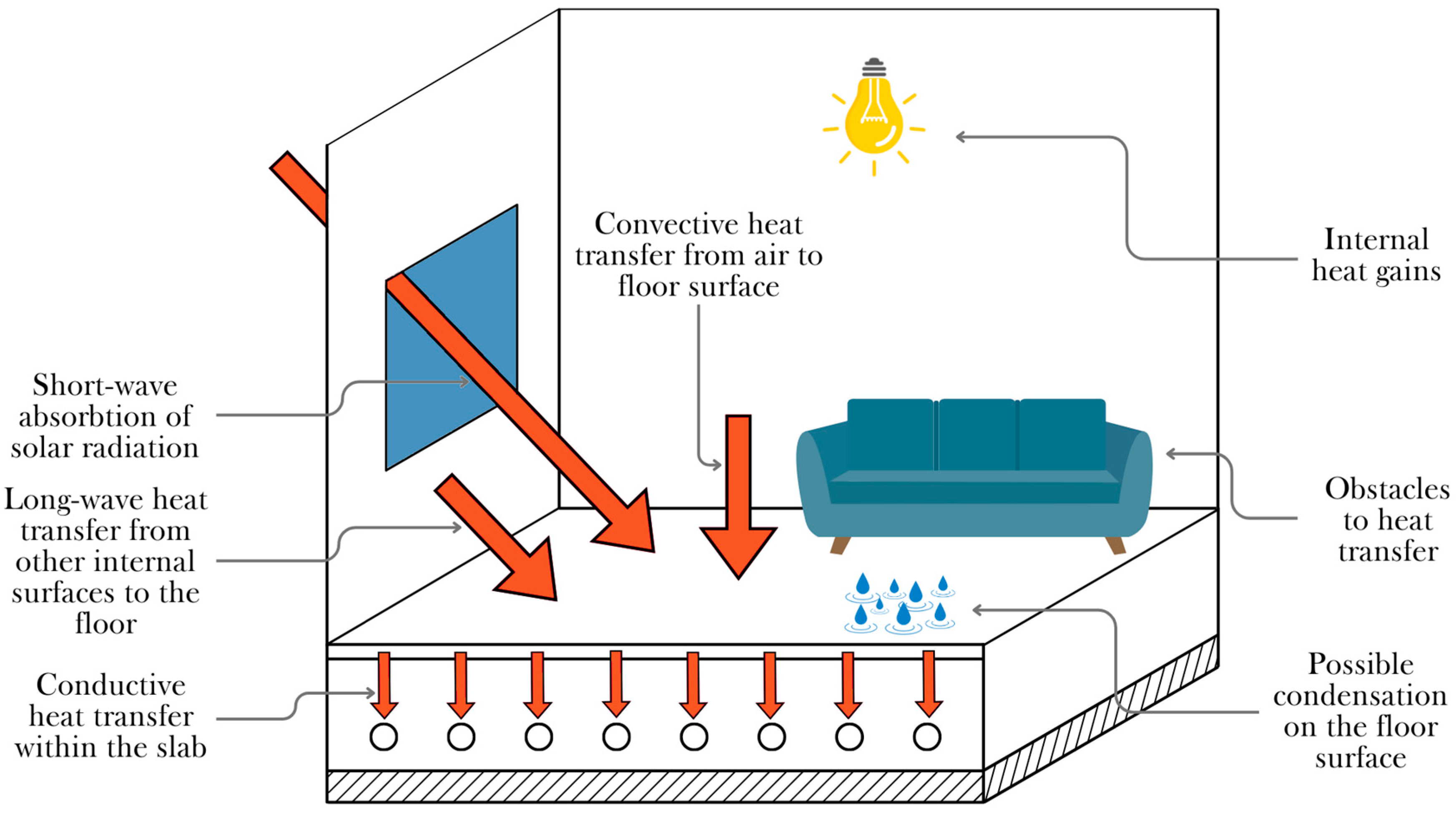
Due to the complexity of heat and mass transfer phenomena, it is common to simplify an analysis by modeling the behavior of a single thermal zone, rather than considering an entire building. The heat transfer mechanism involved in radiant floor cooling can be simplified as follows: first, the chiller produces cold water that is circulated through pipes buried in the floor. As the cooled water flows through the tubing, it cools the slab, while heating itself in the process. Conduction within the floor cools the surface, which in turn transfers heat by convective and radiative processes. Specifically, the cooled surface interacts with the ambient air through convection and also cools internal surfaces such as people, furniture, and walls through radiant heat transfer. The latter is the main mechanism by which the floor exchanges heat. Additionally, the radiant floor is also capable of removing internal and solar heat gains from the room, reducing their direct influence on the indoor air temperature. The phenomena and contributions considered to have the greatest influence on system performance are presented in Figure 1.

As stated above, an important operational issue is the possibility of condensation on the floor surface, which occurs when the temperature reaches the dew point limit. This is indeed a major problem with radiant systems, which can only handle the sensible heating/cooling load without removing the latent fraction. Even though the present study does not directly address the condensation phenomenon, this issue is one of the main drivers of the research, as modeling methods for the floor surface are particularly suited for its avoidance.

Accordingly, this review primarily aims to provide an in-depth analysis of the methods discussed and employed in scientific publications on radiant systems modeling. Our specific focus is on radiant floor cooling models; however, we have also included models designed for other types of TABS or ESS terminals, e.g., chilled ceilings or heated floors, which could also be suitable for floor cooling modeling purposes. To the best of our knowledge, no previous review paper has offered a specific analysis on the topic. Thus, it is essential to conduct a comprehensive study not only to highlight the limitations and possibilities of particular models that may be suitable for research, industrial, or technical purposes, but also to identify and outline the possible existing gaps in the literature related to the modeling of these systems.

The paper consists of seven other sections, in addition to this preliminary introduction. The following chapter explains the methodology employed to categorize the models and presents the main criteria used to describe specific methods. The subsequent two chapters, respectively, explore the models used for floor conduction and the more comprehensive modeling strategies that consider the coupling between the floor and the rest of the thermal zone. Then, the focus shifts to specific submodels for heat transfer mechanisms that have a significant impact on the description of TABS behavior. Finally, before some critical consideration of the accuracy of the models and the conclusive remarks, Section 6 examines the modeling methodology used in software and international technical standards.

2. Methods

As previously stated, RFCS can be a very useful solution for energy efficiency in buildings, and their modeling is a key phase that allows the full exploitation of their potential in specific applications. Consequently, a comprehensive survey of the modeling methods of RFCS proposed in the literature so far can provide a deeper understanding of the state of the art and address what still remains unfulfilled.

The scientific papers analyzed and discussed in the present review proposed modeling methods for TABS that were considered suitable for the purpose of modeling RFCS. The reviewed papers were published within the time span of 1990–2023, which corresponds to the phase of the vigorous revival of radiant systems as heating or cooling terminals in the building sector. The bibliography research was primarily conducted on the Scopus database by searching in the article title, abstract, and keywords the terms “radiant system”, “TABS”, “model”, and “simulation” and then selecting the actual papers that proposed an original model for thermally activated building radiant systems. References of previously identified papers have subsequently been screened for additional material to add to the present review. Finally, further searching on Google Scholar was conducted with the same keywords so as to include papers not published in Scopus-indexed journals.

From the previously outlined bibliography research, 28 scientific papers coherent with the analyzed topic were identified. These are therefore the major focus of the present review.

The most intensive production of modeling techniques considered applicable to floor cooling configurations began in 2003, but there has been no clear growth trend since then. The timeline of the published papers on this topic is shown in Figure 2.

To concisely assess the load of information from the publications, a word cloud chart was employed as a helpful tool to outline the key points common to the majority of the publications. Figure 3 shows the word cloud derived from the analysis of the abstracts of the 28 reviewed papers after removing non-significant terms such as conjunctions, articles, and so on. In the cloud, each word is presented with a font size that is linked to the number of occurrences in the texts under consideration. As could be expected, the most common words were those closely related to the main subject of this paper, such as “model”, “floor”, “cooling”, “radiant”, “surface”, “temperature”, “system”, “heating”, “thermal”, “panel”, and others. Since these terms were not considered significant hints for the survey, they have been hidden from the word cloud in order to place greater emphasis on aspects potentially useful for the models’ classification.

The so-modified diagram thus reveals a great relevance of terms such as “method”, “simplified”, “dynamic”, “steady”, “air”, “validated”, “experimental”, “analytical”, “numerical”, “performance”, “comfort”, “design”, “two-dimensional”, “capacity”, “RC-network”, and many more. These keywords provided a helpful guideline for the analysis of RFCS modeling methods.

Indeed, one of the main goals of our study is the classification of the models available in literature. The first and major distinction among models is shaped by the target phenomenon being modeled. Most of the analyzed works focused on the study and representation of the conductive exchange within the radiant slab, considering the rest of the building, i.e., the other internal surfaces of the room and the air temperature, as fixed boundary conditions that are not thermally affected by radiant or convective heat transfer with the floor. In these models, the focus is placed only on the conductive mechanism occurring within the floor slab, which is justifiably considered the most interesting and peculiar aspect to be modeled. Consequently, the majority of RFCS modeling methods fall into this category. On the other hand, other models consider the comprehensive coupling between the TABS and the rest of the building, and they are thus able to fully represent the behavior of the assessed room as it is subjected to specific climatic conditions. The latter class of methods is especially suitable for carrying out complete dynamic simulations of the cooling performance of the entire building system. That said, these comprehensive models are more general methods which may include the former ones, or similar methods, as a description of the conduction within the floor and then integrate them with the description of other passive building elements.

Another classification scheme for RFCS concerns the modeling method itself: even among the more commonly used white-box techniques (i.e., physics-based approaches), different modeling strategies can lead to a wide range of results in terms of accuracy, computational time, and modeling complexity. Therefore, it is fundamental to distinguish between numerical, analytical, and semi-analytical (e.g., RC) methods. In addition, gray-box and black-box techniques may be used to represent the dynamic behavior of TABS, integrating or substituting the physical explanation of involved phenomena with the analysis of datasets acquired during the operation of the system.

Additional important features highlighted in the present review are the spatial dimensionality of the analysis, the temporal dependency, the methodology used to validate RFCS models, and the purpose aimed at. Finally, the original application for which the model was developed is also illustrated. A schematic representation of the proposed classification methodology is presented in Figure 4. This classification was partly based on the previous results of the word cloud analysis.

Different modeling approaches allow a more or less accurate description of the system, but an extremely precise evaluation of TABS behavior is not always needed, as it may be useless for the purpose of the application. This issue will be discussed in more detail later on.

As shown by Figure 4, there is also an additional class of models that focuses on indoor air modeling, assessing air movements and possible temperature stratification within the analyzed room [39,40,41,42], whose use is usually limited to detailed occupants’ comfort evaluations. However, these models are not available for radiant floor cooling applications yet. They are normally used for radiant systems integrated with air systems (e.g., chilled ceilings integrated with displacement ventilation), which are beyond the scope of this review paper. That is why they were not previously introduced and will not be examined in the following sections.

The hereafter discussed modeling methods also differ in the way in which they account for other important phenomena involved, such as the convective exchange from the floor and the indoor air, the effect of solar radiation entering the room through glazed components, and additional internal heat inputs. A special focus is given to these collateral effects as well, underlining their implications and discussing different sub-models introduced in the literature.

In the two subsequent sections, in addition to tables presenting a schematic and structured representation of the review’s outcomes, a novel application of Sankey diagrams—commonly used to illustrate tangible flows such as energy—is employed to enhance the clarity and readability of the modeling classification.

Most of the investigated methods have been embedded in in-house simulation programs that have been uniquely designed to run these methods. Although the codes can be executed using different computational languages, this detail is often considered non-essential and consequently omitted from the papers.

3. Models for Floor Conduction

Heat conduction within radiant floors or other TABS has become an attractive research topic since the recent revival of this type of system. The heat transfer process involved in their operation is not trivial, meaning the aim of most of the available models is to find the right trade-off between simplification and descriptive accuracy. The heat transfer taking place within the floor is intrinsically three-dimensional because it involves the exchange between an array of pipes or coils arranged in a specific configuration, in which the temperature varies along their length. Conduction within the screed is also generally a three-dimensional phenomenon. However, the dimensionality of the model could be, and often is, reduced with appropriate assumptions and simplifications.

In the present section, 21 modeling methods for the conduction within the slab are presented and discussed. In these models, the heat transfer with the rest of the room is considered, but the air volume and surroundings are taken as fixed boundary conditions and are thus not affected by the actual floor operation.

A preliminary analysis of the Biot number for a reference floor cooling application shows that the use of lumped models is not fully justified for the floor, since its value is mildly high, as calculated in (1) for a typical case. Therefore, some kind of temperature distribution of the floor should generally be accounted for in order to correctly describe the heat transfer mechanism. The here-calculated floor Biot number is evaluated by taking a typical value of the thermal conductivity of the screed ${\mathsf{\lambda }}_{\mathrm{f}}=1.4\frac{\mathrm{W}}{\mathrm{m} \mathrm{K}}$, whereas the heat transfer coefficient for the surface is taken as an overall value, accounting for both convective and radiant exchange, ${\mathrm{h}}_{\mathrm{c}+\mathrm{r}}=6.5\frac{\mathrm{W}}{{\mathrm{m}}^2\mathrm{K}}$ [43]. The Biot number is then

$${\mathrm{Bi}}_{\mathrm{f}}=\frac{{\mathrm{h}}_{\mathrm{c}+\mathrm{r}}{\mathrm{L}}_{\mathrm{c}}}{{\mathsf{\lambda }}_{\mathrm{f}}}=0.23,$$

(1)

where the characteristic length of the floor was taken as a typical thickness of the screed: ${\mathrm{L}}_{\mathrm{c}}=0.050 \mathrm{m}$. However, in the specific case of a radiant floor, in which the heat path is not exactly in the vertical direction, this choice of characteristic length seems arguable. Indeed, considering the longest path followed by the heat flux, ${\mathrm{L}}_{\mathrm{c}}$, would be a better approximation that also takes into account the horizontal displacement due to heat conduction in between the pipes. Therefore, in our opinion, a meaningful evaluation of ${\mathrm{L}}_{\mathrm{c}}$ should be: ${\mathrm{L}}_{\mathrm{c}}=\sqrt{{\mathsf{\delta }}^2+{\mathrm{L}}^2/4}$, where $\mathsf{\delta }$ is the thickness of the screed and $L$ the spacing among pipes. Considering $\mathsf{\delta }=\mathrm{L}/2=0.050 \mathrm{m}$, the Biot coefficient comes out as ${\mathrm{Bi}}_{\mathrm{f}}=0.33$. Alternatively, the internal resistance could also be directly calculated with an analytical expression, e.g., considering a conduction shape factor. Similar results are obtained with this choice as well.

This analysis shows that in conventional radiant floor applications, as well as those with a more tailored choice of characteristic length, the external resistance is dominant, although it is a situation just at the edge of the applicability of the lumped capacitance approach.

Specifically, for the cooling of a plate, Glicksman and Lienhard [44] report that a lumped capacity solution for the time at which the plate reaches 95% completion of a transient is 3% accurate for $\mathrm{Bi}<0.1$ and 12% for $\mathrm{Bi}<0.5$. With this in mind, the choice of a lumped capacity method as RFCS model should be carefully conceived, as it may cause a significant deviation from exact results.

3.1. Analytical Methods

The developed models were initially mostly analytical. These methods are based on the analytical exact solution of the heat equation. Obviously, simplifications of geometry and boundary conditions must occur.

Early attempts to systematically describe the conduction within TABS were based on previously acquired knowledge of other systems. Indeed, Antonopoulos outlined in his work [11] a one-dimensional analytical model for radiant cooling panels, adopted from previous studies on solar collectors. Despite its simplicity, it allows the determination of the temperature field between tubes, which was validated with more accurate numerical simulations. The study also proposed three parameters to synthetically assess the performance of a specific cooling panel: a coefficient representing the temperature distribution in the flow direction, the panel efficiency, and the mean temperature of the panel. An additional early modeling attempt is the one presented by Kilkis et al. [12], in which the steady-state heat transfer within the panel was schematized using previously developed basic heated slab conduction models to obtain its temperature distribution. Specifically, the temperature variation on the panel surface is determined using the composite fin model, thus allowing the calculation of the maximum and minimum floor surface temperatures. The authors justified the use of a stationary approach by taking into account the significant thermal mass of the panels, which enabled a quasi-steady state analysis to be performed. The model has been validated on ANSYS numerical results, reporting a $0.2 °\mathrm{C}$ variance in the calculation of the average floor temperature. The application context for which this steady-state method was conceived is that of design calculations. A more ambitious three-dimensional analytical approach for multi-layer floors was developed by Simões and Tadeu in [16], where the heat transfer problem within the slab was solved using Green’s functions in the frequency domain. This approach enables, at the cost of considerable mathematical complexity, the determination of the entire temperature distribution in the floor in transient conditions without the computational effort needed by numerical methods. However, the pipes are considered linear thermal sources/sinks; therefore, the effect of their dimension is neglected. Additionally, Flores Larsen et al. [17] developed a radiant floor model based on mathematical techniques to solve 2D heat transfer equations within TABS. Using the separation of variables approach, they initially obtained the steady-state solution and then superimposed the unsteady temperature variation. Then again, considering the hypothesis of a slow temperature drop along the pipe, the heat transfer in the third dimension was modeled independently of the other two. The main drawback of this work is the absence of a validation of the method. Such an approach to integrate the analysis of an additional spatial dimension is frequently employed in slab models, as in Li et al.’s paper [29], which also employs the separation of variables technique, and in other models subsequently assessed. Previously, Li and colleagues had made another attempt to model multilayer radiant floors [22], but they limited their results to the two-dimensional temperature distribution.

Consequently, analytical models are highly valuable for representing system behavior without overburdening the calculation process.

3.2. Numerical Methods

Numerical works are based on numerical methods for the solution of partial differential equations (i.e., the heat equation); they offer a highly accurate representation of the studied mechanisms without the simplifying requirements of analytical methods. The heat transfer phenomena may be fully represented with steady-state or transient methods in two or three dimensions. On the other hand, numerical approaches generally require significantly higher computational effort, and results are very case-specific without providing general insights that can be easily extrapolated to analogous cases. In this context, three research studies based on numerical simulation methods are presented.

The development of a finite volume method (FVM) and its use in steady-state simulations was conducted by Jin et al. in [18] for floor cooling applications. Assuming a small temperature variation along the buried pipe, the heat transfer phenomenon within the floor was reduced to two dimensions in order to easily assess the effect of the thermal resistance of the pipe and water velocity. Remarkably, in the assessed configuration, the ignored resistance of a plastic pipe is reported to cause a $0.7 °\mathrm{C}$ error on the floor surface temperature estimate, whereas in case of metal pipes, the error is negligible. They also evaluated the effect of different water velocities and found a $0.5 °\mathrm{C}$ error in surface temperature estimates with plastic pipes. Likewise, Su et al. developed a two-dimensional steady-state numerical model, but of the finite difference type (FDM) [25]. Their study is specific to concrete ceiling cooling panels, but is potentially applicable to floor cooling as well. In the assessment, they also evaluated the effect of pipe spacing on temperature non-uniformity at the floor surface. As might be expected, doubling in the pipe spacing from $150 \mathrm{mm}$ to $300 \mathrm{mm}$ caused a significant increase in the floor surface temperature variation; with an average temperature of $16.2–16.3 °\mathrm{C}$, the largest temperature difference in the latter condition was more than $1 °\mathrm{C}$, while the former condition caused a smaller difference of $0.1 °\mathrm{C}$. Finally, a 3D model was developed by Radzai et al. [30] and used to compare different pipe positioning possibilities through FVM, finding the best temperature uniformity with a two-inlet-two-outlet counterflow serpentine. The model was implemented on Ansys Fluent software. In summary, due to the high computational cost required for the solution of thermodynamic and fluid dynamics equations in each cell of the domain, numerical methods are not suitable for transient simulations. Indeed, these tools are limited to detailed design and comfort evaluation and are not suitable for predicting actual TABS energy performances.

3.3. Semi-Analytical Methods

Finally, semi-analytical methods are the last major category of RFCS models here discussed. They represent some combination of analytical and numerical approaches, and this hybrid nature enables them to efficiently simplify the description of such intricate systems, which are quite hard to describe analytically, making them more practical and feasible to handle. Among others, this category includes resistance-capacitance (RC) models, in which the heat transfer equations are simplified to treat the problem with a lumped approach. RC models are considered semi-analytical because of the technique used to characterize the lumped parameters R and C, which is often analytical. Conceptually, however, they are similar to numerical methods.

A significant number of developed radiant systems models fall within this class. Several configurations of resistance-capacitance networks are possible, such as the ones investigated in [13,15,20,31]. Shmidt and Johannesson’s [13] work developed a form of numerical modeling technique composed of macro-elements, each described with a simplified RC network, which greatly relieves calculation complexity compared with classical numerical methods. The values for thermal resistors and capacitors were calculated from the geometric and thermal properties of the configuration. Their analysis was carried out in the frequency domain using a MathCad environment, and was subsequently validated with an analytical solution. Then, the more recent paper by Zheng et al. [31] also proposed a model where the ground is discretized into a reasonable number of elements, each containing a single section of the pipeline, and each of which is described by an RC network, where the solar contribution is also considered as a current generator placed in each enlightened surface node. To validate the method, an electrical heating film was placed on the floor to simulate the influence of solar radiation. A case study was also simulated to evaluate the effect of unevenly distributed solar radiation. The results showed that a uniform distribution of solar radiation leads to an underestimation of the surface temperature in the irradiated zone and an overestimation in the shaded zone. The model application showed that, due to the impact of solar radiation, local surface areas can experience temperatures up to $8.5 °\mathrm{C}$ higher than the non-illuminated zones.

Weber and Johannesson [15] proposed yet another alternative approach, using a single core node to represent the entire floor. This method calibrates the RC network, studying both star and delta configurations, based on the results of finite element simulations; the network is established between the buried tube and the top and bottom spaces. A similar method is the one developed by Liu and coworkers [20], who were able to estimate the values of the resistances and capacitances of the network with no need for additional simulations; the values to be assigned to RC parameters were derived from geometrical and thermal properties.

Many other semi-analytical methods approximate heat transfer in radiant panels in a simpler manner, only accounting for steady-state conditions. In these situations, the RC network is reduced to a combination of resistors, connecting nodes at a constant temperature. Jin et al. [19] applied such a methodology to describe radiant floor systems, but to characterize the floor performance more thoroughly, they obtained a correlation for the thermal conductivity of the layer with embedded tubes from numerical simulations, assessing its dependance on pipe diameter, spacing, thermal conductivity of the immediately above layer, and conductivity of the pipe. This need for additional simulations was then addressed by Zhang et al. [21], who also proposed a method for estimating the temperature variation on the floor surface that is only dependent on thermal and geometric parameters. Their research has yielded yet another valuable result, the so-called “attenuation coefficient”, which is a metric to characterize the relationship between the warmest and coldest spots on the floor surfaces: $\mathrm{S}=\frac{{\mathrm{T}}_{\mathrm{surf},\max }-{\mathrm{T}}_{\mathrm{surf},\min } }{{\mathrm{T}}_{\mathrm{supply}-{\mathrm{T}}_{\mathrm{return}}}}.$This coefficient can be easily calculated using a proposed correlation, providing valuable insight for various applications, such as condensation prevention. An additional simple thermal resistance series was used by Li et al. [23] to schematize the heat transfer within the floor, from the pipe to the air node, to assess the influence of different floor structure characteristics, i.e., pipe spacing and depth of embedded pipes. Furthermore, a steady-state conduction model applicable to RFCS, which does not require additional simulation for parameter estimation, was developed by Wu et al. [26], who used the conduction shape factor—specific for an array of pipes—to correct the thermal resistance representing the screed. Their model was validated using both measured data and numerical simulations performed with the HEAT2 program. For heating applications, the maximum errors between the model and experiments were $0.8 °\mathrm{C}$in terms of average surface temperature and $8.1 \mathrm{W}/{\mathrm{m}}^2$ in terms of heat flux.

Nonetheless, in addition to models based on the RC analogy, other semi-analytical methods are available in the literature. For instance, Laouadi [14] overlapped a one-dimensional numerical solution, calculated from an energy simulation software, with an analytical temperature perturbation in the other direction. The model is thus able to return a simplified bi-dimensional and transient temperature distribution within the floor. Another methodology called the “reaction coefficient method” was used by Tian and colleagues [24] to describe the behavior of an RFCS. Their unsteady model simplified the heat transfer in the slab and was found to be able to correctly model the system, at least under the stationary conditions in which the validating experiment was carried out. The last semi-analytical model here analyzed was developed by Merabtine et al. [28]. It simplifies the process with a basic exponential equation representing the temperature trend in time, which is calibrated on results deriving from a more accurate numerical model. Although this model does not explicitly incorporate the whole physical behavior of the system, validation against experimental results yielded deviations of the average surface temperature within $2.4\%.$

3.4. Data-Driven Methods

Further, while the previously presented papers focused on white-box techniques that physically represent the system behavior, black-box methodologies are also available. These approaches do not require any prior knowledge of the system, but simply exploit input and output parameters recorded during past system operations. Qin et al.’s work [27] falls within this category, being based on fuzzy logic. The variables which are measured and analyzed in order to estimate the indoor temperature in a room with an RFCS are external air temperature and relative humidity, indoor air temperature for autoregression, and supply and return water temperatures.

Data-driven methods are indeed a promising technique for modeling complex systems, such as radiant floor cooling systems. These methods could be used effectively in a variety of scenarios, even in cases where limited information is available about the case study. However, they need a vast amount of operational data, and because they do not take physical elements into account, their accuracy may decrease, especially when alterations are introduced to the system.

3.5. Overview of the Methods

To summarize, despite the existence of a wide variety of methods, similar features are traceable in many models. For instance, an important feature is how the model handles the heat flow along the pipework. A common approach is to consider a single average temperature for the fluid all along the pipework and subsequently calculate the temperature distribution along the pipe by applying thermal balance equations to a portion of the fluid. These equations are solved as decoupled from the main solution, and this simplification is justified by the reduced temperature gradient along the pipe, which allows the conductive heat transfer in the longitudinal direction to be neglected without committing significant errors.

Regarding the fixed boundary conditions (BC) employed, a common approach is to use a third type of BC for the surface nodes. Two heat transfer coefficients could be used to separately account for different mechanisms. The radiant coefficient (${\mathrm{h}}_{\mathrm{r}}$) is used to schematize the radiant exchange towards the mean radiant temperature of the surroundings, whereas the convective coefficient (${\mathrm{h}}_{\mathrm{c}}$) accounts for the exchange with air. Alternatively, a single coefficient, ${\mathrm{h}}_{\mathrm{c}+\mathrm{r}}$, might be employed to characterize the combined heat transfer with the room operative temperature. In all the cases analyzed in this section, both the heat transfer coefficient and ambient temperature are assumed as constant and not related to the dynamic RFCS operative conditions.

Table 1. Comparison of modeling methods for floor conduction in radiant cooling systems. NA: not applicable; n.a.: not available; n.s.: not specified.

Reference	Methodology	Dimensionality	Time Dependency	Validation	Applicability Context	Purpose
Antonopoulos [11]	Analytical	1D	Steady-state	Numerical	Ceiling embedded piping	Correlation development
Kilkis et al. [12]	Analytical	1D	Steady-state	Numerical	Heating/cooling panels	Design calculations
Simões and Tadeu [16]	Analytical	3D	Unsteady	Numerical	Floor heating	Performance assessment
Flores Larsen et al. [17]	Analytical	2D (simplified approach for 3rd dimension)	Unsteady	n.a.	Floor heating/cooling	Benchmark for models validation
Li et al. [29]	Analytical	2D (simplified approach for 3rd dimension)	Steady-state	Experimental (2D) and numerical (3D)	Floor heating/cooling	Performance assessment and optimal design
Li et al. [22]	Analytical	2D	Steady-state	Experimental	Floor heating/cooling	Performance assessment
Jin et al. [18]	Numerical (FVM)	2D	Steady-state	Experimental	Floor cooling	Design calculations
Su et al. [25]	Numerical (FDM)	2D	Steady-state	Experimental	Chilled ceiling	Design calculations
Radzai et al. [30]	Numerical (FVM)	3D	Steady-state	Experimental	Cooling panels	Design calculations
Schmidt and Johannesson [13]	Semi-analytical (RC)	3D	Unsteady	Analytical	Heating/cooling TABS	Integration in energy software
Zheng et al. [31]	Semi-analytical (RC)	3D	Unsteady	Experimental	Floor heating	Design and control
Weber and Johannesson [15]	Semi-analytical (RC)	1D	Unsteady	n.a.	Heating/cooling TABS	Performance assessment
Liu et al. [20]	Semi-analytical (RC)	1D	Unsteady	Numerical	Cooled panels	n.s.
Jin et al. [19]	Semi-analytical (R)	1D	Steady-state	Experimental	Radiant panels	Design calculations
Zhang et al. [21]	Semi-analytical (R)	1D	Steady-state	Experimental	Floor heating/cooling	Design and performance calculations
Li et al. [23]	Semi-analytical (R)	1D	Steady-state	Experimental	Floor cooling	Design calculations
Wu et al. [26]	Semi-analytical (R)	1D	Steady-state	Experimental and numerical	Floor heating/cooling	Design and control
Laouadi [14]	Semi-analytical	1D (simplified approach for 2nd dimension)	Unsteady	Numerical	Radiant panels	Integration in energy software
Tian et al. [24]	Semi-analytical	2D	Unsteady	Experimental (only steady-state)	Floor cooling	n.s.
Merabtine et al. [28]	Semi-analytical	0D	Unsteady	Experimental	Heating panels	Control applications
Qin et al. [27]	Data-driven (Fuzzy logic)	NA	Unsteady	Experimental	Floor cooling	Control applications

presents and structures the details of the previously disclosed methods for slab conduction modeling in RFCS.

The outcome of the review of this modeling class reveals a great variety of methods, covering almost every possible combination of characterizing features. Each method has its own unique characteristics that can be considered advantages or disadvantages depending on the specific application for which it is intended. For example, analytical methods require little computational effort, making them suitable for applications where computational capacity is limited or where short simulation times are required. However, since the mechanisms described are not trivial to treat, they usually rely on simplifications and approximations that may undermine the accuracy of the model. On the other hand, numerical methods may aim at more detailed and accurate descriptions of the system behavior, but at the cost of higher computational resources required and a high specificity of the solution. Finally, semi-analytical models represent a blend of both numerical and analytical characteristics. They are able to provide detailed representations of case studies without overburdening the calculation process, but they often rely on physical simplifications that may not lead to accurate results.

However, as also discussed in Section 7, it is unreasonable to seek a universal model that will be suitable for all applications. The pros and cons of each method will only become clear once the specific model requirements are established.

As useful tools to better understand the outcome of the review, Figure 5 and Figure 6 concisely summarize the interconnections between the different modeling features. In fact, Sankey diagrams are here used to represent, with the width of each flow, the number of models that embody both the specific starting and arriving characteristics; therefore, each flow represents the number of models that follow that specific path.

In this regard, Figure 5 represents the subdivision of the modeling approaches concerning the dimensionality of the method. Interestingly, the graphic highlights that the most used modeling methodologies, i.e., semi-analytical, mainly employ a one-dimensional description of the problem, significantly simplifying its solution. However, semi-analytical approaches are also suitable for more detailed analysis, in spatial terms, as well as for deeply schematic 0D models. On the other hand, numerical methods are mainly used where a detailed description of the problem is involved; thus, they have been only used for two- or three-dimensional analysis. The fully analytical methods were used in 1D studies as well. Regarding the purposes of the methods, the most remarkable observation arising is that, for design scopes, simplistic 1D models are typically employed, since no high geometric resolution is actually needed in the design phase.

Analogously, Figure 6 illustrates yet a different Sankey diagram focusing on the temporal nature of the description, i.e., whether it is steady-state or transient. As expected, all numerical methods perform steady-state analysis, since they would require a too-high computational effort to study the transient behavior of the TABS. Instead, the unsteady analysis is mostly performed with semi-analytical methods, which mainly employ RC networks, which are indeed a practical modality to study the transient behavior of such systems. Steady-state models were mainly proposed for design calculation purposes, since the sizing of HVAC systems is usually based on a worst-case scenario—which is considered with stationary analysis—whereas transient methods were mainly used for control applications—in which a complete and dynamic model might be needed—or for other purposes, e.g., integration in energy software.

At this point, a brief discussion of the characteristic time values for typical radiant systems becomes appropriate. Indeed, such an indication might help us to understand the importance of the transients undergone by the system. The conference paper by Ning et al. [45] provides a broad evaluation of the thermal time constant for radiant systems, which is the time needed by the system to reach the $63.2\%$ portion of a step change. Considering a step change at the start-up of the system, with an initial equilibrium condition in which the floor is at the set-point room temperature, they reported a wide variety of time constants depending on the type of radiant systems. For commonly used TABS or ESS, time constants are in the range of $3–7$ $\mathrm{h}$, but a variation in the pipe spacing or depth of the screed could deeply influence these results. However, such a general indication is still useful to underline the prolonged time intervals needed by the system to reach steady-state. Since normally the boundary conditions vary as well, the steady-state condition may never actually be reached. Another important effect of the high thermal time constant is that classical control applications face a relevant delay when trying to adjust the system operation, as the effect of the control action will be observed hours later. Therefore, the integration of a reliable model in the control devices may help to overcome this significant time lag, as in the case of model predictive controllers.

4. Coupled Floor-Building Models

Despite conductive heat transfer being the most noteworthy and peculiar aspect of RFCS modeling, to adequately describe their behavior in a built environment, heat exchange with air and other internal surfaces should also be accurately characterized. Especially if the model is intended for application in dynamic building energy and comfort simulations, it is important to employ a comprehensive modeling methodology that can also evaluate the impact of the floor surface cooling on other internal surfaces and air. Indeed, the behavior of these passive elements significantly influences both comfort and energy performance as well.

Therefore, while the previously discussed class of models is particularly suitable for the optimal design of the emitting terminal—focusing on specific behaviors of the radiant floor—the coupled floor-building models are the best way to perform simulations of whole systems, especially those indicated for integration in control applications or just to perform realistic energy and comfort assessment on specific case studies.

Nevertheless, there are a few models in the literature on radiant systems that consider the interactions between the active radiant surface and other passive elements in the thermal zone. Specifically, for the purpose of this paper, seven such models have been identified. The least recent is Lim et al.’s [32], where a complete model was developed to simulate the effect of different HVAC control methods. They used a one-dimensional unsteady FDM numerical approach, and the heat transfer within the cooled floor was schematized through the effectiveness-NTU and fin efficiency methods. For all the walls in the room, they considered conductive heat transfer, convection with air, radiant heat transfer among other internal surfaces, and the effect of solar irradiation. The modeling phase included in their research is only preparatory to the assessment of different control strategies for RFCS, which is the main focus of the paper. Another comprehensive method was proposed by Henze et al. in [33], where they presented a TABS model used to simulate the performance, both in terms of energy and comfort, of a radiant system with assisted ventilation. The model was obtained using an energy software (TRNSYS—Transient System Simulation Tool) which was then modified with a simplified approach for TABS: the active layer was considered to reach the desired set-point with a first-order dynamic, with a time constant fitted to the experimental results for a specific building. Subsequently, in 2012, a new complete numerical method called DIGITHON was presented by De Carli et al. [35], specifically developed for the thermal balance of rooms with radiant systems. It subdivides the room into elemental nodes, but not as densely as in classical numerical methods, to relieve computational effort. For each node, the complete heat transfer mechanism is considered, and good accuracy is confirmed by experimental results. However, to apply the model, previous numerical simulations, with greater computational complexity, must be carried out to characterize the simplified behavior of each node. An interesting finding of the study was also the sensitivity analysis of convective heat transfer coefficients, both in heating and cooling applications. The results showed that there were no notable differences in the calculated air temperature when comparing a variable coefficient, derived from measured values, with a constant coefficient taken from the EN 1264 standard [46].

The RC-network methodology is also effectively employed in coupled models, since, besides the active floor, it is also extremely suitable for passive wall characterization. In Zhang et al.’s [36] and Grassi et al.’s [34] works, and likewise in the more recent publication by Lu et al. [38], RC complete models were developed for an entire examined room equipped with radiant panels. Zhang’s and Lu’s models simplified the heat transfer mechanism by merging the passive surfaces in a single node, whereas Grassi’s method separately considered the effect on each wall, representing each of them with a passive RC network. Instead, the active node—the one with TABS—was schematized with methods similar to the ones treated in the preceding section for conduction. In particular, Zhang’s model is specific for lightweight radiant systems and studies a configuration where the pipes are enclosed in an air gap within the floor. In Grassi’s TABS model, a conduction shape factor is used to account for multidimensional effects, and the temperature gradient along the pipes is also considered to effectively estimate the floor surface average temperature. The model was implemented in a Matlab environment. Finally, Lu’s approach involves the schematization of each layer in a multilayer floor with a one-dimensional RC network, in which the exchange between the pipe and the floor is schematized with a core node. The code was tested with several case studies, in which the outdoor air temperature profile was selected from meteorological data in EnergyPlus software. Studying both continuous and intermittent operation, it was recognized that the ratio of radiant floor to unheated surfaces has a significant effect on the thermal output of the radiant panel.

Whereas the previously presented comprehensive models are suited to unsteady applications, Wang et al.’s [37] model was developed for steady-state simulations, considering a combination of thermal resistances. Here the other passive surfaces are modeled with yet another approach, extracting, from TRNSYS simulations, the relationship for the enclosure temperature, depending on indoor air temperature, floor temperature, and external disturbances.

Given the above, a basic similarity among the proposed models can be noted. They combine classical models for building simulation with radiant panels, using modeling methods similar to the ones seen in the previous section. The main differences lie in the integration between these two systems and also in the phenomena accounted for in modeling, e.g., solar radiation, which is even neglected in some studies. Therefore, the modeling complexity does not expand significantly compared to floor modeling alone, mainly because the methodology used to schematize building passive nodes is typically the same already used for the active element. The only additional complexity is indeed the consideration of interactions among different elements, which, however, can be simplified according to the desired accuracy. The main features of each comprehensive modeling methodology are summarized in

Table 2. Comparison of coupled floor-building modeling methods for radiant cooling systems.

Reference	Methodology	Time Dependency	Validation	Applicability Context	Purpose
Lim et al. [32]	Semi-analytical	Unsteady	Experimental	Floor cooling	Control application
Henze et al. [33]	Semi-analytical	Unsteady	Analytical	Heating/cooling TABS	Performance assessment and control
De Carli et al. [35]	Numerical	Unsteady	Experimental	Radiant panels	Performance assessment
Zhang et al. [36]	Semi-analytical (RC)	Unsteady	Experimental	Lightweight heating floor	Design considerations and comfort assessment
Grassi et al. [34]	Semi-analytical (RC)	Unsteady	Numerical	Heating/cooling panels	Design and performance assessment
Lu et al. [38]	Semi-analytical (RC)	Unsteady	Experimental	Floor heating	Performance assessment
Wang et al. [37]	Semi-analytical (R)	Steady-state	Experimental	Coupled radiant floor and air cooling systems	Design and control applications

.

In Table 2, differently from the previous section, no indication is given about the spatial dimensionality of the analysis, since such an indication is deemed to be of no concern in the whole simulation of the thermal zone, in which the three-dimensional nature of the analysis is intrinsic. A summarizing Sankey chart is here reported with an emphasis on time-dependence only, as shown in Figure 7.

As the rendering outlines, most of the coupled floor-building models are semi-analytical and dynamic. Indeed, the RC methodology is particularly suitable to perform transient simulations of the floor and also of the passive elements of the room. These simulations were then mainly used to evaluate the performance of the radiant systems in specific configurations. However, the floor-building coupled models were meant for design and control purposes as well.

Especially in the case of these integrated floor-building models, it is also very important to include the dynamic behavior of the air moisture within the thermal zone. In fact, as previously stated, condensation on the floor surface is a phenomenon to be avoided under all circumstances, so modeling the moisture content is fundamental to foresee and prevent the occurrence of this process. In most applications, a simple lumped moisture balance is sufficiently accurate.

Unless the singularity of condensation occurs, the moisture balance equation can be solved independently of the heat transfer equation, as the effects of the water mass balance on the temperature field are negligible, at least for the level of accuracy aimed at in macroscale building applications. Given that, a simple additional equation should be added to models to monitor the humidity evolution in the room and eventually to control it with additional devices. Considering the inside of the thermal zone as the control volume, the moisture balance takes the form:

$${\mathrm{M}}_{\mathrm{eff},\mathrm{air}}\frac{\mathrm{d}{\mathsf{\omega }}_{\mathrm{i}}}{\mathrm{dt}}={ \stackrel{·}{\mathrm{m}}}_{\inf }\left({\mathsf{\omega }}_{\mathrm{out}}-{\mathsf{\omega }}_{\mathrm{i}}\right)+{ \stackrel{·}{\mathrm{m}}}_{\mathrm{vent}}\left({\mathsf{\omega }}_{\mathrm{vent}}-{\mathsf{\omega }}_{\mathrm{i}}\right)+\sum { \stackrel{·}{\mathrm{W}}}_{\mathrm{g}}-\sum { \stackrel{·}{\mathrm{W}}}_{\mathrm{c}}$$

(2)

where ${\mathsf{\omega }}_{\mathrm{i}}$, ${\mathsf{\omega }}_{\mathrm{out}}$, and ${\mathsf{\omega }}_{\mathrm{vent}}$ represent the humidity ratio of the thermal zone air node, of the outside environment, and of the air flow entering through the air ventilation systems, respectively. ${ \stackrel{·}{\mathrm{m}}}_{\inf }$ and ${ \stackrel{·}{\mathrm{m}}}_{\mathrm{vent}}$ are the infiltration and ventilation mass flows, whereas ${\mathrm{M}}_{\mathrm{eff},\mathrm{air}}$ is the effective air node mass, which may include a corrective coefficient to simulate the effects of the buffered humidity. The last two terms indicate the generation of humidity (${\stackrel{·}{\mathrm{W}}}_{\mathrm{g}}$), possibly due to people, cooking, and water uses, and the moisture sink (${\stackrel{·}{\mathrm{W}}}_{\mathrm{c}})$, caused by the occurrence of condensation. The latter term includes both undesired events, such as the condensation on the floor surface, and intentional moisture removal by terminals designed to handle latent loads, e.g., dehumidifiers or fan-coils. The formation of condensation occurs when the local air temperature drops below the dew point temperature; this phenomenon can be studied through the use of the Carrier diagram. This is a standard methodology normally employed in building simulation, and generally a conservative approach should be used to compensate for uncertainties in the solution of the temperature field.

Therefore, sufficiently high supply temperatures should be used to keep the floor surface above the dew point temperature and prevent condensation. Control strategies should include a modeling method capable of determining the minimum floor surface temperature and, consequently, the most appropriate supply temperature from the chiller. Models that consider the floor surface as a single node are thus inadequate for this purpose, unless a corrective approach is used to determine the minimum temperature from the average surface temperature.

More accurate moisture modeling techniques also account for sorption effects, whether with a simple correction for air mass—with a corrective multiplying factor $>1$—or with a more detailed description of moisture uptake and release by walls and other objects in the thermal zone.

5. Analysis of Key Modeling Aspects

Besides the conductive heat transfer within the radiant slab, other modeling aspects acquire an essential role in the correct estimation of the whole system performance. Among them, the presence of solar radiation, the convective exchange with air, and the longwave radiative exchange with other internal surfaces are acknowledged as the most significant, as they directly influence the temperature of the radiant floor. Additionally, the effect of humidity within the room also has important implications for the system operation, as previously mentioned.

Solar heat gain is an important contribution to be considered in energy performance analysis and becomes particularly relevant in cooling applications. With radiant cooling systems, this gain can be directly removed by the active surface without warming the air in the first place. As mentioned earlier, this is one of the main advantages of using radiant systems as emissive terminals, and it is especially true for floors, since they usually are an internal opaque surface that is more subjected to direct solar radiation. Consequently, as signaled by several studies on the matter [47,48], when solar radiation is present, the cooling capacity of the TABS is increased. Thus, being acknowledged as an important matter in radiant systems operation, modeling strategies for the solar radiation effect have been intensively studied. For instance, the focus of Causone et al.’s analysis [49] was to determine the direct solar load on the floor, which is defined as the share of the total solar heat gain entering the room that is directly removed by the TABS. The fraction of the total gain was obtained by means of many simulations for different configurations and results were summarized in graphs to be used in specific cases. In another study, De Carli and Tonon [5] carried out a thorough investigation to determine the level of precision required to accurately account for solar radiation in energy simulations. They compared four models with different levels of approximations and ran their simulations on the previously cited DIGITHON model [35]. Their findings show that, to accurately predict the local thermal behavior of the radiant floor, a detailed model is needed, but if the aim is a broad calculation of the overall cooling performance, little differences are present among different methods. Moreover, a dynamic assessment of the effect of solar radiation by Zhao et al. [50], performed through FDM, showed the increase in cooling capacity when radiation is present and provided a further calculation method to estimate the dynamic temperature trend on the floor surface. Similar goals as Zhao’s were pursued by Feng and coworkers in [51], in which they used EnergyPlus as a simulative tool. An additional study by Tang et al. [52] assessed an approach generally used in many modeling methods, which is the even distribution of the solar heat gain on all of the TABS surface as a single node to represent the radiant panel. Their study simulated and compared the uniform distribution approach and detailed 3D assessment, showing reduced errors both in steady-state and transient simulations.

In TABS operation, in addition to the shortwave radiation from the sun, the infrared exchange amongst internal surfaces is also crucial, as it is the main mechanism by which an RFCS cools the environment. This aspect may be modeled with several strategies as well, employing different approximation levels. Two main approaches are usually employed: the mean radiant temperature (MRT) one, in which the heat exchange between the floor and other surfaces is simplified by using a single temperature representative of all the other passive surfaces, and complete methods that consider the amount of absorbed and emitted radiation in each single room surface.

While longwave radiation remains the primary mechanism employed by TABS to maintain occupants’ comfort, it is also essential to acknowledge the significant role of direct convective exchange with air, which thus requires proper characterization. In floor cooling applications, this exchange is typically weak due to the cooled surface being placed at the bottom, which causes air stratification and hinders convective cells that would create air movement within the room. However, that is true only from a strictly theoretical point of view, with two facing plates placed in an infinite medium; in that case, as reported in major heat transfer textbooks, the heat flow in the air medium is entirely conductive, as there would be no motion in the fluid. Despite this, in practical scenarios, numerous instabilities initiate air movements due to the presence of temperature differences. The causes for those thermal movements may include non-uniformity in cooled floor temperatures due to pipe spacing or partial sun insolation, as well as differences in temperature between the floor and other surrounding surfaces, such as walls, people, devices, or furniture. In order to perform a fully detailed analysis, the modeling would have to be extremely tailored to the specific configuration, obviously causing a questionable loss of generality. Additionally, specific devices could be used to enhance the convection within the thermal zone, such as ceiling fans, and such tools might have a significant effect on the energy performance of RFCS [48]. Therefore, with so many specific behaviors and configurations that influence the process, providing a broad and reliable assessment of convective heat transfer is challenging. However, given its minor contribution, simplistic approximations may be tolerable in modeling methods.

A first analysis of the heat transfer coefficient for stratified convection in air can be traced back to the experimental studies on downward-facing heated surfaces [53,54,55,56,57], which are also a useful indication for the analogous case of upward-facing cooled surfaces, as happens in floor cooling applications.

Instead, Olesen et al. [58] developed an experimental study specifically intended to measure the convective coefficients for floor cooling applications. They compared their results with correlations in the literature: Glent [59], ASHRAE fundamentals [60], and McAdams [61]. Their results disagreed with previous studies, showing a higher heat transfer coefficient. However, these results may depend on the specific conditions present in the experimental room, such as wall temperatures. Another in-depth study on the convective exchange between air in a room and a radiant floor, also in cooling applications, was devised by Cholewa et al. [62]. Similarly to the abovementioned article, employing an experimental campaign, convective coefficients for heated/cooled radiant floor in a test chamber were evaluated. The outcome of the study is a general suggestion to decrease the values usually considered as heat transfer coefficients, since they are acknowledged to overestimate actual performances. Yet another equation for the modeling of convective heat transfer in RFCS applications was formulated by Karakoyun et al. in their experimental investigation [63]. Unlike other studies, they included the effects of sidewall temperatures in their analysis and proposed a correlation for the total heat flux by interpolating the results of different configurations of heat gains through the walls. It has the peculiarity of suggesting a negative correlation of the convective coefficient with temperature. Although it goes in the opposite direction compared to other modeling methods, it still seems justified, since an increase in the temperature difference would reinforce the stratification and thus decrease the convective heat transfer.

Finally, the value proposed by the European Standard EN 1264-5 [43] may also be used to characterize convective heat transfer. The convective contribution can be estimated from the total value by subtracting the radiative heat transfer coefficient, calculated as ${\mathrm{h}}_{\mathrm{r}}=4{\mathsf{\sigma }\overline{\mathrm{T}}}^3 {\left(\frac{1}{{\mathsf{\epsilon }}_{\mathrm{floor}}}+\frac{1}{{\mathsf{\epsilon }}_{\mathrm{walls}}}-1\right)}^{-1}$, with ${\mathsf{\epsilon }}_{\mathrm{floor}}$ and ${\mathsf{\epsilon }}_{\mathrm{walls}}$ being the thermal emissivity of the floor and the surrounding walls, respectively.

Above all, an explanation of the progress in the description of convective heat transfer mechanisms, also in floor cooling applications, is given by Camci et al. in [64].

Table 3. Correlations and values of the air Nusselt coefficient usable for the cooled floor surface (stratified conditions). Where not stated, the reference temperature is the bulk temperature.

Reference	Nusselt Coefficient [−]	Notes
Fishenden and Saunders [53]	$\mathrm{Nu}=0.25{ \mathrm{Ra}}^{1/4}$	$3\times {10}^5\le \mathrm{Ra}\le 3\times {10}^{10}$
Min et al. [54]	$\mathrm{Nu}=0.071{ \mathrm{Ra}}^{0.255}$	$Ra$ range not specified
Restrepo and Glicksman [55]	$\mathrm{Nu}=0.587{ \mathrm{Ra}}^{1/4}$	Horizontal heated place facing downwards with cooled sides, $1.66\times {10}^6\le \mathrm{Ra}\le 3.19\times {10}^6$
Alamdari and Hammond [56]	$\mathrm{Nu}=0.586{ \mathrm{Ra}}^{1/5}$	$\mathrm{Ra}<{10}^{11}$
Awbi and Hatton [57]	$\mathrm{Nu}=2.353{ \mathrm{Ra}}^{0.133}$	$1.02\times {10}^{10}\le \mathrm{Ra}\le 7.12\times {10}^{10}$
Olesen et al. [58]	$\mathrm{Nu}=0.654{ \mathrm{Ra}}^{1/4}$ *	$\mathrm{Reference} \mathrm{height} \mathrm{for} \mathrm{air} \mathrm{temperature:} {\mathrm{h}}_{\mathrm{ref}}=0.6 \mathrm{m}$	$2.4\times {10}^{10}\le \mathrm{Ra}\le 5.2\times {10}^{10}$
	$\mathrm{Nu}=0.499{ \mathrm{Ra}}^{1/4}$ *	$\mathrm{Reference} \mathrm{height} \mathrm{for} \mathrm{air} \mathrm{temperature:} {\mathrm{h}}_{\mathrm{ref}}=1.1 \mathrm{m}$
	$\mathrm{Nu}=184.6$ *	$\mathrm{General} \mathrm{suggestion}, {\mathrm{L}}_{\mathrm{c}}=4.8 \mathrm{m}$
Glent [59]	$\mathrm{Nu}=0.265{ \mathrm{Ra}}^{1/4}$ *	$\mathrm{Ra}$ range not specified
ASHRAE [60]	$\mathrm{Nu}=0.230{ \mathrm{Ra}}^{1/4}$ *	$\mathrm{Ra}$ range not specified
McAdams [61]	$\mathrm{Nu}=0.27{ \mathrm{Ra}}^{1/4}$	$3\times {10}^5\le \mathrm{Ra}\le 3\times {10}^{10}$
Cholewa et al. [62]	$\mathrm{Nu}=6$ *	$4.6\times {10}^8\le \mathrm{Ra}\le 1.8\times {10}^9$$, {\mathrm{L}}_{\mathrm{c}}=1.56 \mathrm{m}$
Karakoyun et al. [63]	$\mathrm{Nu}=161.8{ \mathrm{Ra}}^{-0.1}$ *	${\mathrm{h}}_{\mathrm{ref}}=1.1 \mathrm{m}$, heated walls, $1.1\times {10}^9\le \mathrm{Ra}\le 8.6\times {10}^9$$,{\mathrm{L}}_{\mathrm{c}}=1.8 \mathrm{m}$
EN 1264-5 [43]	$\mathrm{Nu}=194.7$	$3.8\times {10}^9\le \mathrm{Ra}\le 5.1\times {10}^{10}$$, {\mathrm{L}}_{\mathrm{c}}=3 \mathrm{m}$ (taken as a typical value)

* In order to represent all correlations in terms of $\mathrm{Nu}$, the values of $\mathrm{g}, \mathsf{\beta }, \mathsf{\nu }$ and $\mathsf{\alpha }$ are calculated for air at $25 °\mathrm{C}$ ($\mathrm{Ra}=9.5\times {10}^7{ \mathrm{L}}_{\mathrm{c}}^3 \mathsf{\Delta }\mathrm{T})$, and, where needed, the characteristic length is retrieved from references by considering ${\mathrm{L}}_{\mathrm{c}}=4\frac{\mathrm{Area}}{\mathrm{Perimeter}}$.

summarizes the values or correlation proposed in the previously mentioned studies to characterize the convective heat transfer coefficient, ${\mathrm{h}}_{\mathrm{s}}$, between the radiant floor surface and the room air node in cooling applications. To easily allow the comparison among different values, all the references are reported in terms of the Nusselt number, $\mathrm{Nu}$, and a general correlation to the Rayleigh number, $\mathrm{Ra}$, can be observed: $\mathrm{Nu}={\mathrm{c} \mathrm{Ra}}^{\mathrm{n}}$. It seems evident that there is no neat agreement on the subject, as the proposed coefficient can differ significantly. This could be seen as an additional demonstration of the fact that convection in floor cooling applications is heavily dependent on site-specific conditions, and therefore it is difficult to propose a general approach with broad validity.

The different correlations are also visually presented in Figure 8. Despite some of them bringing similar results, probably because of similar conditions employed in the studies, a wide range of Nusselt values is actually covered.

Moreover, the study on the convective heat transfer coefficient for heated surfaces in a room carried on by Awbi and Hatton [57] might also be a suitable tool to estimate the convective flux that generates above floor portions that are heated by sun radiation. Indeed, their study includes a focus on partially heated surfaces, from which they conclude there is little difference, regarding the convective coefficient, between a partially and a wholly heated floor.

The above-cited phenomena are the ones acknowledged to have a significant impact on the description of RFCS. However, as previously mentioned, their effect may strongly depend on the actual configuration of the room. For instance, a major difference in the thermal behavior of the cooled space would be caused by the presence of furniture or other comparable obstacles. Their effect not only reduces the long-wave radiation heat transfer but also undermines convective exchange and adds further thermal capacities. This aspect is extremely case-dependent as well, and this is probably the reason why limited studies on the subject were undertaken. The effects of the presence of “light” furnishing (desk, two chairs and a small chest) were experimentally assessed by Wallentén [65], who reported limited effects on convective coefficients. However, that might have been due to the presence of particularly minimal furniture in the room. Subsequently, a fundamental contribution to the subject was given by Fontana in her experimental study on a case model [66] with radiant floor heating. Two different clusters of furniture were assessed in steady-state conditions. Both high and low furniture, representing the distance of the base of the objects from the floor, were reported to have a significant effect on the floor performance, with a reduction in the heat transfer up to 25% for the higher furniture and 30% for the lower one. Nonetheless, it would be too ambitious to take this as a general indication, as many aspects can vary from one situation to another. In addition, as this is a scale study, it is not certain that the results are consistent with real applications. On the other hand, the investigation undertaken by Wolisz et al. [67] focused on the different outcomes of dynamic thermal building simulations due to the presence of floor coverings or furniture. They state that the presence of these supplementary items slows down the dynamics of the building, also quantitatively characterizing it for the specific configuration assessed. Their final recommendation is therefore to incorporate these elements in energy simulations.

Therefore, despite the availability of numerous papers on the subject that recognize the importance of furniture in the performance of radiant floor systems, no general approach has yet been proposed for its implementation in models. The same applies to the convective mechanism: despite many studies and proposed correlations, a comprehensive approach that fully considers the effect of different boundary conditions is not yet available for floor cooling applications. These gaps highlight significant areas that need to be addressed for the development of reliable models of RFCSs.

6. Models Used in Software and Technical Standards

6.1. Software

Software for energy performance evaluations of buildings or other systems is widely used in the thermal engineering field nowadays, both for research and industrial purposes. Its application in energy simulations is crucial for optimizing systems operations towards energy efficiency. The two most commonly used softwares are TRNSYS, already mentioned, and EnergyPlus, an open-source simulation program developed and freely distributed by the U.S. Department of Energy.

The two above-cited software are able to perform complete dynamic simulations of building energy behavior, with the possibility of including radiant floors as emissive sub-systems as well. Performing complete simulations, their modeling logic is similar to the one described in Section 4 of the present review because they provide thermal coupling between the models of the radiant panel and the rest of the thermal zone.

The conductive model on which EnergyPlus is based is the transfer function method [68,69]. Two separate models for radiant systems are available, a one-dimensional method and a more detailed two-dimensional method; the heat exchange between the tube and the floor is then schematized in both approaches with the epsilon-NTU approach, as already seen for several other TABS models. The 1D method was validated in a successive study by Chantrasrisalai et al. [70]; however, a more recent paper by Brideau et al. [71] questioned the EnergyPlus correct estimation of the conductive heat transfer within the floor, comparing the output of its simulations with reference finite elements analysis. After an appropriate tuning, the 2D code was found to be coherent with the benchmark solution, whereas the 1D solution caused relevant deviations from the actual solution. Nevertheless, EnergyPlus and its model for radiant embedded systems are often renovated [72], and present concerns will be reasonably gradually corrected.

On the other end, the TRNSYS simulation software provides three distinct modeling methods for TABS, which were validated and compared in a study by Rey et al. [73]. The first approach is the active layer method that is integrated into “Type 56”, which is the TRNSYS model for a general built environment with multiple thermal zones. The active layer model used for TABS was developed following Glück’s method [74], which establishes a conduction network using a correction similar to the conduction shape factor approach. Then, the flow direction is also considered to take into account the temperature variation along the pipe. This resistive approach is employed for steady-state calculations but is also regarded as valid for transient conditions. No detailed documentation is available for the other two TRNSYS modeling methods, which are the so-called “Type 653” and “Type 993” methods. However, as indicated in their description in the user manual, the former one is a model with features similar to the one included in “Type 56”, considering the floor as a lumped capacitance and modeling the heat transfer between the tube and the floor with a heat exchanger approach. Instead, the latter is a more detailed modeling method that operates a 3D analysis of the conduction within the TABS; therefore, it requires a relevantly larger computational effort. “Type 993” was reported to be the least accurate method, whereas the two lumped approaches were able to predict the temperature within the pipes and the surface temperature more correctly. However, the outputs of the models are particularly dependent on several input parameters which are hard to know exactly; therefore, the correct estimation with the last two methods was obtained after a tuning process on those parameters.

Besides the fundamental description of the conductive mechanism within the floor, calculation software such as TRNSYS and EnergyPlus also consider all the other phenomena involved in the thermal balance of the studied zone. Among them, the thermal linkage between the floor and other internal surfaces and also the air node are considered. Furthermore, the crucial effects of solar radiation and internal gains are also modeled. The two programs describe these phenomena in different ways, and each of them also accepts the use of different levels of modeling accuracy, giving the choice of a more detailed method or a simplified one.

Thus, the models included in these software packages do not introduce any significantly novel element compared to the models discussed in the previous sections. In fact, the techniques used in their simulations suffer from the same limitations: either the description is too simplistic and struggles to provide accurate results or it is too detailed, making it impractical for real-world case studies where users may not know the full configuration details. In addition, even though these software tools account for many of the important phenomena, they still have the same problems as other modeling methods in terms of convective exchange and accounting for furniture.

Therefore, it is important that new research developments in modeling methods gradually find their way into simulation software as well. This would allow the improvement of these tools and the wider use of more reliable models.

6.2. Standards

The importance of credible modeling of radiant systems, both in heating and cooling applications, is acknowledged as crucial by international technical standards, which suggest their use both in the design stage, utilizing steady-state analysis, and during the operation of the system, optimizing the system control strategy to improve its energy efficiency. For the latter, dynamic simulations are considered a fundamental tool.

The most relevant international standard concerning TABS is ISO 11855 [75], and, in addition to that, EN 1264 [46], a European standard that deals in detail with the production aspect of radiant panels, is also of interest. ISO 11855 consists of seven parts, with modeling aspects mainly considered in parts two and four. ISO 11855-2 deals with the determination of the thermal heat flux to be given to or removed from the conditioned space by the radiant panel; indeed, it is only focused on steady-state calculations. It suggests the use of numerical methods, for which, however, no indication is given of the special features of the model to be adopted. However, the standard includes a benchmark for model validation. Furthermore, it also provides some simplified methods to model the stationary energy performance in specific configurations.

On the other hand, ISO 11855-4 treats dynamic methods for heating/cooling capacity calculations. It presents four different modeling strategies that differ both in their complexity and in the accuracy aimed at. Besides two roughly simplified methods that estimate the capacity of the TAB system based only on the daily heating/cooling demand, the standard suggests and provides an FDM to model the panel and the room in which it is installed. Additionally, the most accurate modeling method is indicated as a detailed simulation with dynamic software, a strategy that is suggested for cases outside the range of validity of the simplified models.

7. Considerations on Modeling Accuracy

Besides the rather clear distinction between the two main model classes, within each category there is no clear distinction in terms of the convenience of different types of heat transfer resolution method. Numerical, analytical, and semi-analytical methods can indeed achieve similar levels of accuracy, as demonstrated by experimental validations where average errors of a few tenths of a degree Celsius are often obtained. However, the use of one method or another may be more or less appropriate in specific cases, depending on the application for which the modeling is required, the computational capabilities available, and the creative effort one wishes to invest in the modeling phase of the specific system.

Simplified methods, such as those that employ a 1D or 2D approach to investigate a section of the floor, or even 0D models that provide a lumped representation of the problem, typically possess general applicability. Indeed, their output is not dependent on specific room dimensions or pipework configurations, such as serpentine or spiral layouts. Consequently, as evident in Figure 5, they are the main source for design and control purposes, thanks to their generality. Meanwhile, the detailed 3D methods, as well as the coupled floor-building models, require more thoughtful tailoring to the specific dimensions and configuration of the room being considered.

Remarkably, it might be useful to further investigate the accuracy actually needed in the use of the RFCS models. As highlighted in previous sections, two of the most common applications are the design and the control of the cooling systems. In both cases, accuracy of a few tenths of a degree might be significantly superior to what is actually required. Indeed, the design calculations aim to develop a system configuration that can fulfill comfort and energy requirements during its operation. However, for obvious reasons, a conservative approach is generally taken at this stage, whereby the capacity of the system tends to be over-dimensioned in order to ensure good robustness even under rare but extreme conditions. In this context, a model that provides accuracies to tenths of a degree would be over-qualified for real needs. Frequently, steady-state considerations are enough in these situations.

On the other hand, for control applications, dynamic and more accurate modeling could be useful to optimize the operation of the system. However, in these cases, the problem lies instead in the ability to correctly assess the actual state of the building and the system during its operation. For instance, these systems controllers are typically based on the measurement of the ambient temperature using a room thermostat; this applies to current installations as well as many methods still in the R&D phase. The problem is then the actual reliability of the temperature measurement made by the thermostat, since its placement in the room or building often does not reflect the actual internal conditions [76]: errors up to $2 °\mathrm{C}$ have been reported in some scenarios. Therefore, using a system model within a control methodology that aims for much higher accuracy could prove useless in this case as well.

Consequently, selecting the appropriate model for the specific application and context in which it will be used is crucial. For example, in situations where very precise control is desired and where special emphasis is placed on correctly estimating the system state variables, a modeling approach capable of achieving high accuracy would be required. Similar considerations apply to all the features previously listed for each model: there is no need to complicate the treatment by introducing a detailed 3D or 2D description if the target uses do not require it, nor is there a need to treat the problem as time-varying if equally significant results can be obtained with a steady-state analysis. This same principle underlies the use of simplified methods to account for the effect of solar radiation, radiative exchange with walls, convective heat transfer, and the presence of furniture.

The analysis just conducted reveals, indeed, the necessity to tailor the complexity and the accuracy of the modeling method to the specific context for which it is needed. However, as in practical and typically faced contexts great accuracy is not expected, in these situations a deeply detailed model, which may also require the need for more detailed simulations to be characterized, as some of the reviewed methods do, risks being worthless.

Therefore, in our view, future research trends should aim at the development of modeling methods that are oriented toward practical and widespread applications. New models should be easy to characterize, depending on a limited number of parameters that could be easily obtained from building construction projects or on-site surveys. That is, they should be simply employable without the need for too-detailed knowledge of the geometrical and constructive configuration of the system. Moreover, the approach to follow should be the integrated one, considering the coupling between the floor and the rest of the building. Although such a target for wider application would probably involve a lowering of accuracy expectations even in coupled models, overall energy benefits could still be achieved, especially if models are used to improve the control methodologies for both existing and new buildings. A valuable tool to address this need for easily characterizable modeling methods could come from a large-scale monitoring campaign involving actual buildings. The collection of operational data from a wide variety of practical applications could facilitate the development of novel gray-box techniques for modeling buildings equipped with radiant floor cooling systems by integrating these data with the existing knowledge of the physical phenomena governing their operation.

Additionally, a significant gap in the available literature on RFCS modeling methods is the absence of some schematization of the furniture and other obstacles to heat transfer, which might deeply interfere with the heat transfer mechanism previously described, as highlighted by preliminary research investigations on the topic. Even the presence of people and additional internal gains are never fully evaluated since, besides being other terms to take into account in the sensible and latent energy balances, they have a significant influence on the floor heat transfer itself due to the thermal plumes they produce, which increase the convective exchange. As a general suggestion for further research, an effective way to address these modeling gaps would be to conduct several dedicated experimental campaigns on the topics, which may provide the most appropriate means to capture physical behaviors and establish correlations or correction coefficients to be integrated into models.

Not considering these effects can severely undermine model accuracy in real-world scenarios. Therefore, further work on the reliable schematization of these effects is needed and should be widely applicable as well.

8. Conclusions

The installation of radiant floor cooling systems in buildings has the potential to significantly reduce energy consumption in comparison to traditional heating and cooling systems. However, to realize their full potential, a proper characterization of their performance is required, which should consider several important phenomena such as conductive, convective, and radiant heat transfer, heat-removal of solar radiation passing through glazing and of internal loads, as well as other factors such as the possible condensation of moisture on the floor surface and the presence of furniture or other obstructions to heat transfer.

In the presented review, a survey of modeling methods for RFCS was provided. The models proposed in the literature were first categorized according to the physical heat transfer phenomenon they sought to describe, and their objectives were also discussed in order to better understand their possible applications. A novel graphical approach based on Sankey diagrams was employed to effectively summarize the main outcomes of the review. Most of the models focused on the representation of the conductive heat transfer process that takes place within the floor, which is the most distinctive and novel trait brought by radiant systems. Therefore, these models may also be very accurate in their description, but to be truly useful in the simulation of case studies—whether for optimal design, control, or performance analysis—they must be integrated with the model of the entire thermal zone, providing the boundary conditions for the TABS model. Nonetheless, how this integration takes place is not trivial and becomes a further crucial part of the modeling phase. In light of that, some research papers have targeted the modeling of the entire building or room in which the RFCS is integrated, allowing the coherent simulation of the whole thermal zone.

Amongst the latter, some methods effectively considered relevant effects, but often disregarded others, such as the presence of solar radiation and the thermal exchange by irradiation between internal surfaces. However, none of the available models provide the possibility of simulating a configuration with furniture, people in the room, or other obstacles to heat transfer. Therefore, future developments should explore the topic in more depth and attempt to provide simple ways to account for these effects in models.

Further progress is also believed to be necessary in the development of modeling methods that are easy to characterize, so that they can be readily used to improve control applications in practical scenarios where limited information about the case study is available.