A New Method for Predicting the Gas Content of Low-Resistivity Shale: A Case Study of Longmaxi Shale in Southern Sichuan Basin, China

Abstract

Low-resistivity shales are widely developed in the Sichuan Basin. The production of low-resistivity shale gas reservoirs ranges from high to low to none. The existing methods for gas-content prediction cannot accurately predict the gas content of low-resistivity shale. This increases the risk of shale-gas exploration. To prove that the random forest algorithm has apparent advantages in predicting the gas content of low-resistivity shale and reducing the risks associated with shale-gas exploration and development, three prediction methods were selected in this paper to compare their effects. The first method is known as the grey-correlation multiple linear regression method. Low-resistivity shale-gas content logging series were optimized using the grey-correlation approach, and then the low-resistivity shale-gas-content prediction model was established using the multiple linear regression method. The second method we selected was the resistivity method. The improved water-saturation model was used to predict the water saturation of low-resistivity shale, and then the gas content of low-resistivity shale was predicted based on the free-gas content and the adsorbed-gas-content model. The random forest algorithm was the third method we selected. Fourteen logging series were used as input data and the measured gas content was used as supervised data to train the model and to apply the trained model to the gas-content prediction. The findings demonstrated that the grey-correlation multiple regression method had poor accuracy in predicting gas content in low-resistivity shale; The resistivity method accurately predicted water saturation, and the predicted gas content was higher than the actual gas content. Because the random forest algorithm accurately predicted low-resistivity shale-gas content, its use in the Sichuan Basin was advantageous. The selection of a low-resistivity shale-gas-content prediction model was guided by the research findings.

1. Introduction

Shale-gas resources are abundant in the Sichuan Basin, which is the primary area for developing oil and gas reserves [1]. However, operational issues arise during the shale-gas discovery and production process. One of the major issues is the discrepancy between the calculated results for low-resistivity shale-gas concentration and the actual test results. The calculation model is directly related to the incorrect estimation of the gas content in low-resistivity shale. Exploiting the link between logging resistivity and the water saturation of a reservoir is the usual practice in calculating the water saturation of shale, the gas saturation of shale, and the gas content of shale [2]. However, pyrite is an additional component that lowers the resistivity of shale in comparison to the resistivity of shaly sandstone and pure sandstone. Over-matured organic matter is another element contributing to lower resistivity in low-resistivity shale than in ordinary shale [3,4]. Low-resistivity shale’s conductive mechanism is more intricate than that of normal sandstone and conventional shale. The standard method of calculating water saturation results in high anticipated water saturation and low gas content [5]. The reserve assessment and the exploration deployment of low-resistivity shale gas are severely hampered by an erroneous estimate of gas content. Therefore, it is critical to consider the techniques for predicting the gas concentration in low-resistivity shale.

There are now two sorts of shale-gas-content prediction systems. The resistivity approach is one. By examining the conductive properties of shale, it is possible to improve resistivity, and the water-saturation-calculation model is then used to forecast shale-water saturation and determine its gas saturation and gas content [6]. The Simandoux equation model, the modified Simandoux equation model, the total shale model, the modified total shale model, the Indonesian model, the dual-water model, and the dispersed-clay model have provided the greatest increases in resistivity and water saturation. These models take into account the effects of clay minerals, clay minerals’ cation-exchange capacity, and unripe organic matter in the formation of resistivity. However, they ignore the effects of pyrite and overripe organic matter on shale resistivity. Therefore, it is necessary to improve the models [7,8].

The non-resistivity approach may be divided into two categories. One category is based on experimental findings, examining the adsorbed-gas-content control elements (such as total organic carbon (TOC), clay mineral content, and the relative humidity of shale) and improving the Langmuir equation [9] and, on this basis, predicting the adsorbed gas content using the logging curve [10]. The free-gas content is obtained by using the logging curve, based on the ideal gas-state equation, and then the predicted adsorbed-gas content and the free-gas content are added to obtain the total shale-gas content. However, the prediction results of this method are significantly different from the measured results when the gas fugacity form is unclear.

The other category of the non-resistivity approach consists of optimizing the density and the compensated neutron curve from the geophysical meaning of the logging curve, then fitting the total gas content by multiple linear regression or the multivariate high-order equation to obtain the total gas content of the shale. However, for types of shale with different compositions, different densities, and inconsistent water saturation, there are differences in the hydrogen-content index determined by compensating neutrons. This makes it difficult to promote the application of this method.

In recent years, with the rapid development of artificial intelligence and big data technology, artificial neural networks, machine learning, and deep learning algorithms have played an important role in various industries [11]. Machine learning has been widely used in the prediction of the bearing of shale gas. The commonly used machine algorithms are the support vector machine regression (SVR) algorithm, the back propagation (BP) neural network algorithm, the random forest (RF) algorithm, the convolutional neural network (CNN) algorithm, and the decision tree (DR) algorithm [12]. The SVR algorithm requires optimization of the model parameters, but the computational time required to use the optimization algorithm is long [13]. BP neural networks are used for coefficient determination by back propagation, which often results in overfitting [14]. CNNs are implemented on the basis of image training and usually require a large number of samples [15]. The random forest algorithm and the decision tree algorithm are effective algorithms for predicting the gas content of shale by obtaining a large dataset with a put-back extraction, and they are able to extract dominant features [16].

By contrasting three shale-gas-content methods—grey correlation and multiple linear regression, enhanced resistivity technique, and random forest—this work demonstrates the superiority and accuracy of the RF machine learning algorithm in estimating low-resistivity shale-gas content to maximize attractive drilling targets.

2. Geology Settings

The Sichuan Basin has generated five basement faults (Figure 1). From west to east, the Sichuan Basin is divided by these basement faults into six secondary tectonic units: western, southwestern, central, northern, southern, and eastern Sichuan [17]. The Lower Silurian Longmaxi Formation shale in the Sichuan Basin is one of these faults and it is primarily found in the western, southern, and eastern regions of Sichuan. The Sichuan Basin has seen multiple stages of tectonic movement since the Longmaxi Formation shale was deposited, including the Hercynian, Indosinian, Yanshan, and Himalayan motions [18].

During the Hercynian movement, due to the influence of the Dongwu movement, the Emei ground fissure activity led to the eruption of basalt along the basement-fault fissure, which affected the distribution of the geothermal field in the Sichuan Basin and had an important influence on the thermal evolution of organic matter in the Longmaxi Formation shale.

During the Indonesian movement, due to the closure of the Paleo-Tethys Ocean, the extrusion activity formed several paleo-uplifts in the Sichuan Basin, including the Luzhou paleo-uplift and the Kaijiang paleo-uplift. The Jiangnan Xuefeng orogenic belt shifted to the northwest during the Yanshan movement period, creating several northeast-trending broom-shaped fold groups and northeast-trending fault systems in the southeast Sichuan region. Additionally, during this time, a significant amount of gas was produced in the Longmaxi Formation shale. A significant right-lateral strike-slip stress field developed in the western Sichuan Basin during the Himalayan period as a result of the Qinghai–Tibet Plateau’s eastward extension, activating the fault system that had been created during the Yanshan period. Shale gas and fluid activities in the southern Sichuan Basin are significantly impacted by the fault system created by the two tectonic movements known as the Yanshan period and the Himalayan period [19].

In a vertical direction, the Lower Silurian Longmaxi Formation can be divided into the first member and the second member of the Longmaxi Formation. The major layer of shale in the Longmaxi Formation that produces gas is known as the first member of the formation. This layer is further separated into the 11th, 12th, 13th, and 14th members of the formation. The southern Sichuan region is situated on the deep shelf or the transition zone between the deep shelf and the shallow shelf during the shale deposition period of Long 1-1. It mostly produces carbonaceous siliceous shale and carbonaceous calcareous shale, both of which have significant levels of organic matter and little variation in the mineral content of the clay [20,21].

3. Data Selection and Methods

The well-location information and the particular methods chosen in this paper are used to establishing that the random forest machine learning algorithm has more advantages than the multiple linear regression method or the resistivity method in predicting the gas content of low-resistivity shale.

3.1. Data Selection

Shale with logging resistivities less than 10 ohm·m is referred to as low-resistivity shale. According to the origin of the shale, it can be separated into four different types of low-resistivity shale: a superheated-evolution type, a high-water-saturation type, a layered-pyrite type, and a bedding-fracture type. The layered-pyrite type of low-resistivity shale is only produced locally and has no impact on the shale’s gas concentration. As a result, it is not taken into account in this study.

Low-resistivity bedding-fracture-type shale is created when mud filtrate enters the fracture, which—in actual geological conditions—is not filled with other materials and has no discernible impact on shale gas content. Therefore, this kind of low-resistivity shale is not taken into account in this study.

The superheated-evolutionary and high-water-saturation type (type I) and the superheated-evolution type (type II) were chosen to thoroughly examine the benefits and drawbacks of the three approaches (the random forest machine learning algorithm, the multiple linear regression method, and the resistivity method). The type I low-resistivity shale of four wells was chosen as the object in the vicinity of the fracture because high water saturation is related to the fracture distance. The four wells were designated A1, A2, A3, and A4, referring to the Tiangongtang anticline, the Luochang syncline, the Linjiang syncline, and the Tiangongtang anticline, respectively. Low-resistivity shale from the A1 through A3 wells was used for training the gas-content prediction model, while low-resistivity shale from the A4 well was utilized for testing the model. Four type II low-resistivity shale wells were chosen as the objects, and they were located far from the fault. These four wells were designated B1, B2, B3, and B4, respectively, in the west wing of the Xiaocaoba anticline, the Huguosi syncline, the Jianwu syncline, and the Yunjin syncline. Low-resistivity shale from wells B1 to B3 was used to train the gas-bearing prediction model. For model testing, the B4 well’s low-resistivity shale was utilized.

Table 1. Each well’s related information of low-resistivity shale of Long 1-1.

Type	Well Name	Vitrinite Reflectivity (%)	Water Saturation (%)	Pressure Coefficient	Mineralization (g/L)
type Ⅰ	A1	3.52	55.00~83.30 (69.38)	1.68	23.35
	A2	3.80	59.19~89.90 (72.93)	0.50	23.57
	A3	3.47	39.95~78.73 (64.07)	1.95	24.65
	A4	3.50	27.90~89.50 (63.82)	1.00	23.94
type Ⅱ	B1	3.60	33.70~56.84 (46.60)	2.00	24.83
	B2	3.52	56.93~70.78 (62.97)	2.05	25.85
	B3	3.39	32.07~78.39 (59.01)	1.90	25.69
	B4	4.59	54.63~62.62 (59.10)	1.00	24.28

Annotation: min~max (average).

displays the pertinent details of the low-resistivity shale in each well.

3.2. Methods

In this study, three methods—the resistivity technique, grey-correlation multiple linear regression, and the random forest algorithm—were used to predict the gas content of low-resistivity shale. Below are the fundamental tenets of the three techniques.

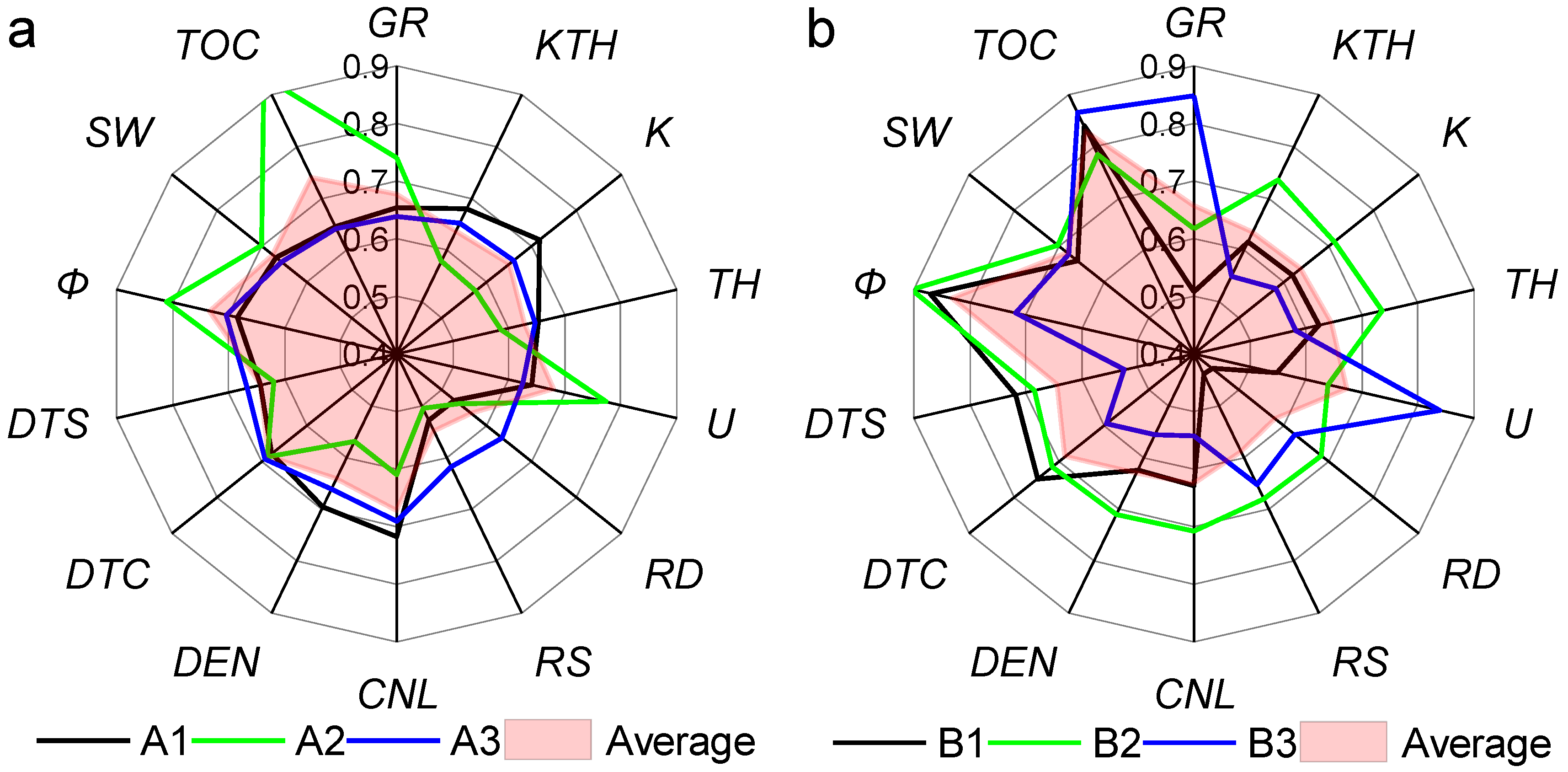
3.2.1. Grey Relational Analysis

Grey correlation analysis is a technique used to gauge how closely two variables are correlated. The degree of correlation between the two elements is strong during the system development process if the trajectories of the two factors are consistent [22,23]. The steps are as follows, according to the core principle of grey relational analysis:

(1)

Each independent variable is represented by a comparison sequence (Xi = xi(k)|k = 1, 2, n) and a reference sequence (Y = y(k)|k = 1, 2, m), while the dependent variable is represented by the reference sequence [24].

(2)

The comparison sequence and the reference sequence are normalized so that each independent variable and each dependent variable have values between 0 and 1.

(3)

The grey correlation coefficient i(k) of each element in each comparison sequence is calculated, based on this information. The calculation formula is as follows:

$${\zeta }_i(k)=\frac{\underset{i}{\min }\underset{k}{\min }|y(k)-x_i(k)|+\rho \underset{i}{\max }\underset{k}{\max }|y(k)-x_i(k)|}{|y(k)-x_i(k)|+\rho \underset{i}{\max }\underset{k}{\max }|y(k)-x_i(k)|}$$

(1)

(4)

The average grey correlation coefficient, or the degree of grey correlation r_i between each independent variable and each dependent variable, is computed for each comparison series. Below is the calculating formula:

$$r_i=\frac{1}{n}{\displaystyle \sum _{k=1}^n{\zeta }_i(k) k=1,2,\cdots ,n}$$

(2)

3.2.2. Multiple Linear Regression

Multiple independent variables are used in multiple linear regression to estimate the dependent variable. The fundamental formula is as follows:

$$y={\beta }_0+{\beta }_1{X}_1+{\beta }_2{X}_2+\cdots +{\beta }_k{X}_k+\mu k=1,2,\cdots ,n$$

(3)

A multivariate linear regression model may then be obtained using the least squares approach by minimizing the sum of squares of the error to identify the optimum function and by performing a matrix operation to generate the coefficient matrix [25,26]. The coefficient matrix equation is as follows:

$${\beta }^{’}={(X^{T}X)}^{-1}{X}^{T}y$$

(4)

3.2.3. Prediction of Shale Gas Content Based on the Resistivity Method

Typically, the Archie formula is used to determine how saturated with water the pure sandstone is, and this application has achieved good results [27]. However, there is some mud in pure sandstone under actual formation circumstances. The logging resistivity will decrease somewhat, due to the mud’s high cation-exchange capacity and additional conductivity, and the water saturation determined by the Archie formula will be high. The majority of studies have recommended an updated Archie formula to determine the precise water saturation of shaly sandstone.

Table 2. Modified Archie models.

Model	Equation	Characteristics
Modified Simandoux	$\frac{1}{R_t}=\frac{V_{sh}{S}_w}{R_{sh}}+\frac{{\varphi }^m{S}_w^2}{a{R}_w}$	Applied to shaly sandstone
Total shale	$\frac{1}{R_t}=\frac{{\varphi }_t^m}{a{R}_w}{S}_w^n+\frac{V_{sh}}{R_{sh}}{S}_w^{n-1}$
Waxman–Smits	$\frac{1}{R_t}=\frac{S_w^n{\varphi }^m}{a}\left(\frac{1}{R_w}+\frac{B{Q}_v}{S_w}\right)$
Dual-water	$\frac{1}{R_t}=\frac{S_w^n{\varphi }_{}^m}{a}\left(\frac{1}{R_w}+\frac{S_b}{S_w}\left[\frac{1}{R_b}-\frac{1}{R_w}\right]\right)$	Modified from the Waxman–Smits model; water in reservoirs is divided into irreducible water and free water.
Indonesian	$\frac{1}{\sqrt{R_t}}=\left(\sqrt{\frac{{\varphi }_{}^m}{a{R}_w}}+\frac{V_{sh}{}^{(1-V_{sh}/2)}}{\sqrt{R_{sh}}}\right)S_w^{n/2}$	Considering the total porosity-containing organic matter is currently the most suitable model for shale.

displays the currently most-frequently used improved formulae.

Table 2 shows that the Waxman–Smits model is more appropriate for reservoirs with ionic double-electron layers on the shaly surface and that the modified Simandoux model and the total shale model are adequate for the water-saturation prediction of shaly sandstone reservoirs [28]. The Waxman–Smits model, which is more appropriate for argillaceous sandstone reservoirs holding bound water and free water, is the basis for the improvement of the dual-water model. Although the model does not take into account the impact of organic matter on resistivity, the existing Indonesian equation for shale reservoirs better describes the non-linear relationship of the shale reservoir conductivity model and is more suitable for conventional shale water-saturation prediction. Therefore, an organic matter term was added to the Indonesian equation and stated that organic matter increases logging resistivity and that the relationship between resistivity and organic matter content is quadratic [29], as shown in Equation (5). However, in low-resistivity shales, both organic matter and pyrite with superheated evolutionary degrees lead to a decrease in shale resistivity. Therefore, Sanjukta’s improved model does not apply to the prediction of water saturation in low-resistivity shale. In this paper, a model for predicting water saturation in low-resistivity shale is proposed by combining the Indonesian model with the Sanjukta model and its concept of a quadratic nonlinear relationship between log resistivity and each conducting material (Equation (6)).

$$R_t=\frac{R_o}{S_w^n}-{(V_{CLAY})}^2\cdot R_{sh}+{(V_{om})}^2\cdot R_{om}$$

(5)

$$\frac{1}{\sqrt{R_t}}=\{\sqrt{\frac{{\varphi }^m}{a\cdot R_w}}+\frac{V_{sh}{}^{(1-V_{sh}/2)}}{\sqrt{R_{sh}}}\}{S}_w{}^{n/2}+\frac{V_{om}}{\sqrt{R_{om}}}+\frac{V_{py}}{\sqrt{R_{py}}}$$

(6)

In the low-resistivity shale water saturation model, the lithological coefficient (a), the cementation index (m), and the saturation index (n) can be obtained by rock-resistivity experiments. The formation-water resistivity can be obtained by Equation (7) and the resistivity (R_sh) of argillaceous can be obtained by logging resistivity in the statistical relationship with clay mineral content; The volume fraction of organic matter may be obtained by Formula (8), and the resistivity (R_om) of organic matter in the degree of superheating evolution may be obtained by the statistical relationship between well-logging resistivity and TOC. Pyrite resistivity (R_py) is obtained via the relevant literature.

$$R_w=\left[\frac{1}{2.74\times {10}^{-4}\times S^{0.955}}+0.0123\right]\times \left[\frac{81.77}{1.8\times T+6.77}\right]$$

(7)

$$V_{om}=\frac{TOC\times {\rho }_b}{{\rho }_{om}}$$

(8)

Based on the accurate calculation of the water saturation (S_w) of low-resistivity shale, the gas saturation (S_g) of low-resistivity shale is calculated by Equation (9) and the free-gas volume (V_f) of low-resistivity shale is calculated by Equations (10) and (11).

$$S_g=1-S_w$$

(9)

$$V_f=\frac{P{T}_{SC}{S}_g\varphi }{ZT{P}_{SC}{\rho }_r}$$

(10)

$$P=\alpha P_{hydrostatic}=\alpha {\rho }_{w}gh$$

(11)

The adsorbed-gas capacity (Vs) of low-resistivity shale can be obtained using the Langmuir equation (Equations (11) and (12)). In the Langmuir equation, the Langmuir volume (V_L) can be obtained by Equations (13) and (14), the Langmuir pressure (P_L) can be obtained from Equations (13) and (15) [30], and Formulas (14) and (15) are substituted into Formula (12) to obtain the calculation model of the adsorbed-gas amount (Formula (16)).

$$V_S=\frac{V_L\times P}{P+P_L}$$

(12)

$$t=t_0+\gamma \times h/100$$

(13)

$$V_L=0.49\times TOC-0.01\times t+2.06$$

(14)

$$P_L=e^{\frac{-1325.43}{t+273.15}+4.8}$$

(15)

$$V_S=\left[\frac{0.49\times TOC-0.01\times t+2.06}{P+e^{\frac{-1325.43}{t+273.15}+4.8}}\right]\times P$$

(16)

The total gas content (V_total) of the low-resistivity shale is obtained by adding the free-gas amount of the low-resistivity shale and the adsorbed-gas amount (Equation (17)).

$$V_{total}=V_S+V_f$$

(17)

3.2.4. Random Forest Regression

The random forest method was created on the foundation of decision trees. It is a supervised machine learning algorithm that is part of an ensemble learning algorithm [31]. The algorithm’s primary phases for implementation are as follows (see Figure 2):

(1)

The dataset is divided into the independent variable matrix and the dependent variable vector (label).

(2)

The same number of samples is pulled from the initial data set, using put-back to create various subsets of the unordered data set [32].

(3)

A decision tree is obtained for each subgroup by using label-supervised learning to identify a certain number of ideal features (shown by the red line in Figure 2).

(4)

The decision trees of each subset are combined to obtain random forests.

(5)

The prediction results of each decision tree are added and averaged to determine the predicted value.

3.2.5. Method Process

For the grey-correlation multiple linear regression method, the logging curve that was sensitive to the gas content of low-resistivity shale was first optimized by the grey correlation method, then the multiple linear regression method was used to establish a relationship between the gas content of low-resistivity shale and the sensitive logging curves. Finally, the fitted relationship was used for the prediction of the gas content of the same type of low-resistivity shale [33].

For the resistivity method, the new water-saturation model was used to predict the water saturation of low-resistivity shale. The prediction results were compared with the measured water saturation, and the model parameters were continuously improved to obtain accurate water-saturation prediction models for different types of low-resistivity shale. On that basis, the free-gas volume and adsorption gas volume prediction models were applied to determine the gas content of low-resistivity shale, and the whole set of models was applied to predict the gas content of the same type of low-resistivity shale.

For the random forest algorithm, the GR, KTH, K, TH, U, RD, RS, CNL, DEN, DTC, DTS, SW and TOC logging curves or the interpretation results from six wells from A1 to A3 and B1 to B3 were regarded as input data and the measured gas content was regarded as supervised data to train a set of gas-content prediction methods applicable to all types of low-resistivity shale. The trained random forest model was used for low-resistivity shale gas-content prediction in other wells.

The gas contents predicted by the three methods were compared with the measured gas contents in wells A4 and B4 to clarify the superiority of the random forest algorithm in the prediction of gas content in low-obstruction shale [34].

4. Results and Discussion

4.1. Prediction Effect Analysis Based on Multiple Linear Regression

For type I low-resistivity shale, that is, superheated-evolutionary and high-water-saturation low-resistivity shale, the correlations between GR, KTH, K, TH, U, RD, RS, CNL, DEN, DTC, DTS, Φ, SW, TOC and gas content were analyzed by the grey-correlation method. The results showed that the logging series with a high correlation with the grey degree of low-resistivity shale gas content of the A1 well included K, CNL, DEN, and DTC, while the logging series with a high correlation with the grey degree of low-resistivity shale gas content of the A2 well included GR, U, DTC, Φ, SW, and TOC and the logging series with high correlation with the grey degree of low-resistivity shale gas content of the A3 well included KTH, K, TH, RD, RS, CNL, DEN, DTC, and DTS. To obtain a unified logging series with a high grey correlation with type I low-resistivity shale gas content, we adopted the method of averaging the grey-correlation degree of each logging series and gas content in the three wells, A1 to A3, and the average value reflected the grey-correlation degree of each logging series and type I low-resistivity shale gas content. Logging series with grey correlation values greater than 0.65 were defined, as well as series that were closely related to low-impedance shale-gas content, which can be used for low-resistivity shale gas-content prediction. Finally, the log series that were closely related to the gas content of type Ⅰ low-resistivity shale were GR, U, CNL, DTC, Φ, SW, and TOC (Figure 3a), and the relationship equation between the gas content of type Ⅰ low-resistivity shale and the log series was fitted by the multiple linear regression method (Equation (18)); the fitted correlation coefficient was 0.73 [6,35,36].

$$\begin{array}{ll}Total Gas Content& =-4.57-0.01\times GR+0.27\times U-0.19\times CNL+0.15\times DTC\\ & -25.77\times \varphi +0.42\times SW-112.45\times TOC\\ & R^2=0.73\end{array}$$

(18)

Repeating the above method, the logging series that were closely related to the gas content of type Ⅱ low-resistivity shale were U, DTC, Φ, SW, and TOC (Figure 3b). Similarly, the relationship between type II low-resistivity shale gas content and the logging series (Equation (19)) was fitted by the multiple linear regression method, and the correlation coefficient of the fit was 0.55, which was lower than that of type I low-resistivity shale.

$$\begin{array}{ll}Total Gas Content& =4.98-0.06\times U-0.08\times DTC+28.91\times \varphi \\ & +0.69\times SW+51.13\times TOC\\ & R^2=0.55\end{array}$$

(19)

It can be seen from Figure 4 that the gas-content and the measured-gas-content data points of type I low-resistivity shale were distributed near the 1:1 line, but when the gas content was greater than 3 m³/t, the gas content predicted by multiple linear regression was lower than the measured gas content (Figure 4a), which may have been due to the difference between the sensitive logging series of the low-resistivity shale gas content of the A2 well and the other two wells (Figure 3a). The gas content of type II low-resistivity shale was far from the 1:1 line (Figure 4b), indicating that the method based on grey-correlation multiple linear regression does not apply to the calculation of gas content of type II low-resistivity shale. This is related to the sensitivity logging series of B1, B2, and B3 low-resistivity shale gas content (Figure 3b).

4.2. Prediction Effect Analysis Based on Resistivity Method

The prediction of low-resistivity shale-gas content based on the resistivity method was divided into two steps. The first step was to calculate the water saturation of low-resistivity shale by using the improved-water-saturation prediction model. In the second step, based on the water saturation of low-resistivity shale, the gas saturation of low-resistivity shale was calculated, then the free-gas volume of low-resistivity shale was calculated by the ideal gas state equation combined with the Langmuir model to calculate the adsorbed gas volume of low-resistivity shale. Finally, the total gas content of low-resistivity shale was obtained [37,38].

Due to the lack of petrographic data in the wells selected for this article, the petrographic data of the low-resistivity shale in well R1, which is near well A2, were used to determine the Archie parameter in the water-bearing saturation equation, considering the similar rock-formation characteristics of the main producing layer of the Longmaxi Formation in the Sichuan Basin. Combining the relationship between formation factor (F) and porosity (Φ) (Figure 5a), the lithology factor a in the water-content-saturation model of low-resistivity shale was 1 and the cementation index m was 1.75 by fitting with Equation (20). Combining the relationship between resistivity increase factor (I) and the water-content saturation (SW) of the two data sets, factor b was 1 by fitting with Equation (21) and the saturation index was 2.1.

$$F=\frac{R_O}{R_W}=\frac{a}{{\varphi }^m}\Rightarrow \lg F=\lg a-m\lg \varphi$$

(20)

$$I=\frac{R_t}{R_O}=\frac{b}{S_W^n}\Rightarrow \lg I=\lg b-n\lg S_W$$

(21)

To determine the resistivity of the wet clay, the statistical method of data was utilized. Due to the large number of factors in low-resistivity shale that can lead to reduced resistivity in logging, it is not appropriate to select low-resistivity shale to determine the resistivity of wet clay [39]. The shale of well R2 was selected for the wet clay resistivity value, and the organic matter in the Longmaxi Formation shale of this well did not lead to a decrease in log resistivity (Figure 6a). Furthermore, the amount of wet clay leads log resistivity to decrease [40]. When the amount of wet clay is 100%, however, the log resistivity value may be equal to the amount of wet clay, and the result is 1.71 ohm·m (Figure 6b).

To determine the resistivity of the over-mature organic matter, the same statistical method of data was used. To measure the resistivity of over-mature organic matter, the shale from well B2 was chosen. According to Figure 7a, the water saturation of the shale in this well did not contribute to the decline in shale resistivity. Figure 7b shows a statistical relationship between good resistivity and TOC, which allowed for the determination of the resistivity value of 1.5 ohm·m for over-mature organic matter.

There is a significant relationship between pyrite resistivity and temperature [41]. Previous studies showed that the value of pyrite resistivity is about 0.1ohm·m at temperatures between 300 and 700 K [9]. The current temperature of the Longmaxi Formation shale in the Sichuan Basin ranges from 300 to 700 K. Therefore, the value of pyrite resistivity in Equation (6) is 0.1 ohm·m.

Based on the determination of the above parameters, the water content saturation was predicted using Equation (6) for type Ⅰ low-resistivity shale and type Ⅱ low-resistivity shale (Figure 8a,b). The water-content-saturation-prediction results and the measured values were closely distributed on a 1:1 line, indicating that the improved water content saturation model applies to the accurate prediction of water content saturation in low-resistivity shale.

Based on the accurate prediction of water saturation in low-resistivity shale, the free-gas volume was first calculated using Equations (9)–(11), then the adsorbed gas volume was calculated using Equations (12)–(16). The current geothermal gradient (γ) in Equation (13) was taken to be 3.0 °C/100 m. Finally, the total gas content was calculated using Equation (17). Based on this method, the predicted gas-content values of type Ⅰ low-resistivity shale and type Ⅱ low-resistivity shale were significantly higher than the measured gas content values (Figure 9a,b). This showed that the existing free- and adsorbed-gas models overestimate the gas content of shale, which greatly increases the risks associated with shale gas exploration and development. Two possible reasons for overestimating the gas content of low-resistivity shale were considered. First, employing the ideal gas equation overstates the quantity of free gas in the shale, since the formation conditions are high temperature and high pressure, and the gas contained in the formation is not ideal. Second, the shale reservoir contains a certain amount of formation water, and the existing models do not account for differences in the capacity of organic matter to adsorb under various thermal evolution degrees. As a result, the predicted total gas content for low-resistivity shale may be overestimated as a result of the overestimation of the adsorbed gas.

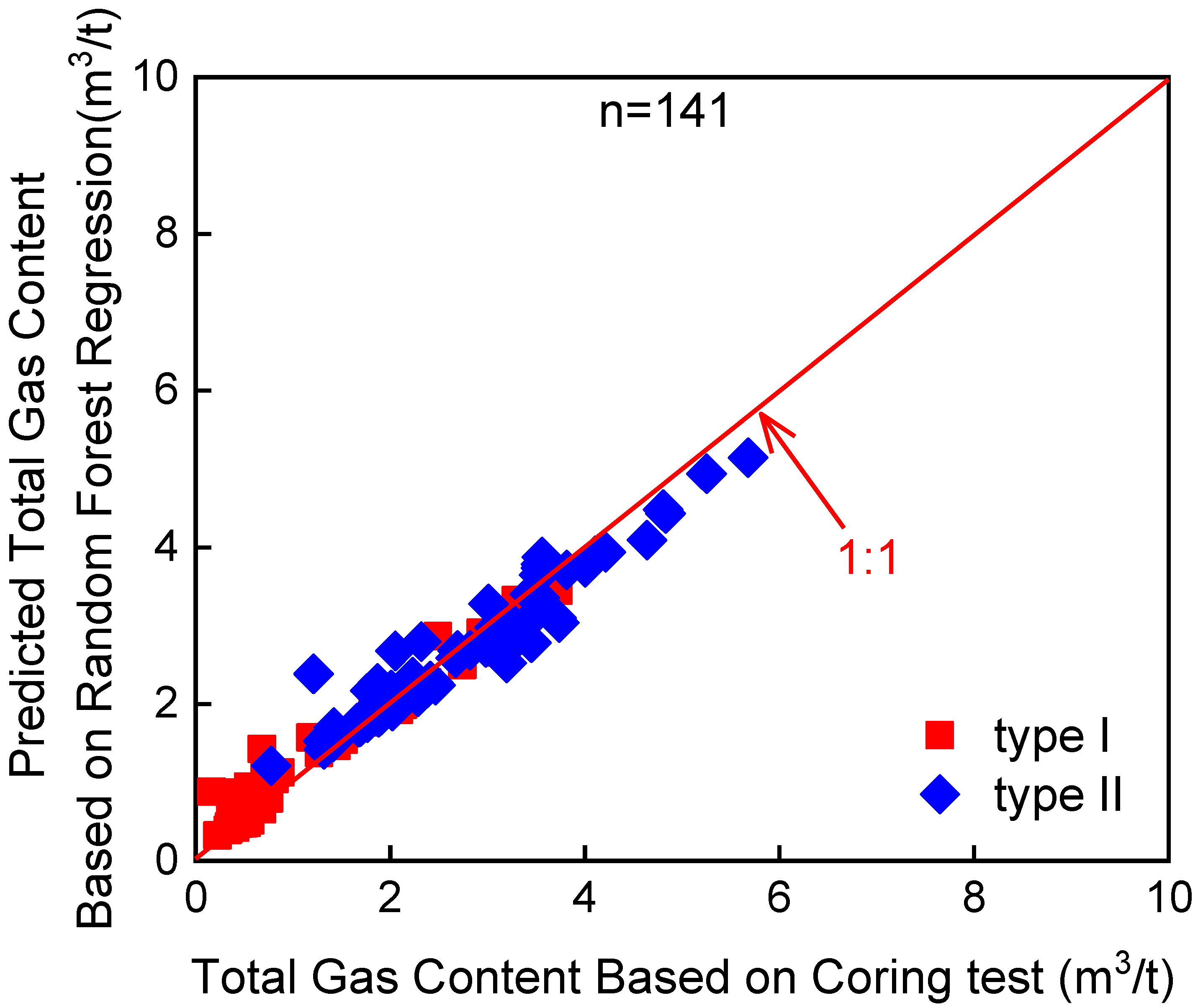
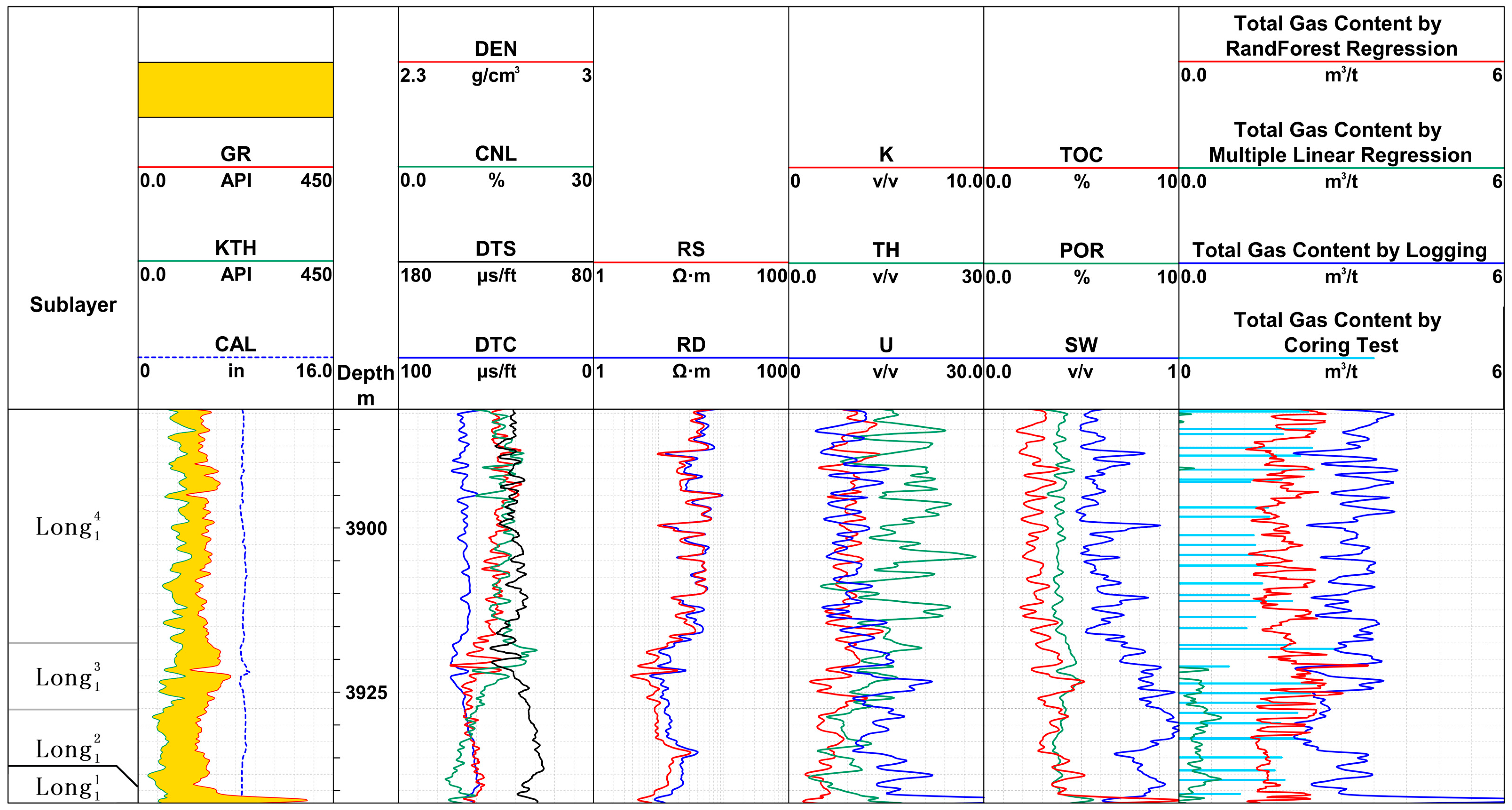
4.3. Prediction Effect Analysis Based on Random Forest Regression

A total of 141 actual measurements of low-resistivity shale gas content from six wells, A1 to A3 and B1 to B3, were used as labels, and 14 attribute values of GR, KTH, K, TH, U, RD, RS, CNL, DEN, DTC, DTS, Φ, SW, and TOC at corresponding depths were used as input data. Using the random forest machine learning algorithm, the original dataset was randomly selected 800 times with all the put-backs, and a total of 800 subsets were obtained. The dominant feature vector (i.e., the decision tree) of each subset was obtained by the supervised training of each subset’s actual measured air content. The gas content of type Ⅰ low-resistivity shale and type Ⅱ low-resistivity shale was predicted using 800 trained decision trees. The results showed that the predicted and measured results were closely distributed on a 1:1 line, and the correlation coefficient between them reached 0.95 with a mean square error of 0.07 (Figure 10). This showed that the random forest algorithm has a great advantage in predicting the gas content of low-resistivity shale, which may be related to the fact that the machine learning algorithm can better learn various characteristics of the data and can fully reflect the influence of an independent variable on a dependent variable.

To verify the validity of the three low-resistivity shale gas-content prediction methods, the type Ⅰ low-resistivity shale of well A4 and the type Ⅱ low-resistivity shale of well B4 were selected for validation. For well A4, the resistivity method’s predicted gas content was significantly higher than the measured gas content, while the trained random forest model’s predicted gas content was in good agreement with the measured gas content. However, the grey-correlation multiple linear regression method’s predicted gas content was significantly lower than the measured gas content (Figure 11). The advantages of the random forest algorithm in predicting the gas content of type I low-resistivity shale were confirmed.

For well B4, the predicted gas content using the grey-correlation multiple linear regression method and the resistivity method was higher than the overall measured value, while the predicted gas content using the trained random forest model was in good agreement with the measured value in the Long₁¹–Long₁³ section (Figure 12). This confirmed the advantages of the random forest algorithm in predicting the gas content of type II low-resistivity shale. As for the Long₁⁴ section, the gas content predicted based on the random forest model was higher than the measured value (Figure 12). This may have been because the training set did not contain all the features of type II low-resistivity shale when the model was trained, so the algorithm did not learn all the features of this type; therefore, inaccurate gas-content prediction occurred in the local-layer section. The characteristic structure of the data will be fully analyzed in a follow-up study to avoid this problem.

5. Conclusions

This paper compared three methods for predicting the gas content of low-resistivity shale. The following conclusions were obtained.

(1)

The gray-correlation multiple linear regression method could not fully include the relationship between the gas content of the two types of low-resistivity shales and the logging series, and the accuracy of the prediction results was low.

(2)

The inclusion of pyrite and over-mature organic matter into the water-content-saturation prediction model was more consistent with the low-resistivity shale petrophysical model. However, the free-gas and adsorbed-gas fugitive forms were not fully defined and the existing free-gas volume and adsorbed-gas volume models could not accurately predict the total shale-gas content, resulting in high prediction results.

(3)

The random forest algorithm comprehensively learned the relationship between the gas content of low-resistivity shale and each logging series. the correlation between the predicted gas content and the measured gas content reached 0.95, which supported the extension of this application in the study area.

References

1. Kokkinos, N.C.; Nkagbu, D.C.; Marmanis, D.I.; Dermentzis, K.I.; Maliaris, G. Evolution of Unconventional Hydrocarbons: Past, Present, Future, and Environmental Footprint. J. Eng. Sci. Technol. Rev. 2022, 15, 15–24. [Google Scholar] [CrossRef]
2. Zhong, G.; Xie, B.; Zhou, X. Shale Gas Logging Evaluation Method—A Case Study of Southern Sichuan Basin. J. Lithol. Reserv. 2015, 27, 96–102. [Google Scholar]
3. Cui, R.; Sun, J.; Liu, X. Study on main controlling factors of low resistivity shale. J. Geophys. Geochem. Explor. 2022, 46, 150–159. [Google Scholar]
4. Sun, J.; Xiong, Z.; Luo, H. Low resistivity genesis analysis and logging evaluation of Lower Paleozoic shale gas reservoirs in Yangtze area. J. China Univ. Pet. (Nat. Sci. Ed.) 2018, 42, 47–56. [Google Scholar]
5. Yin, S.; Ding, W.; Huang, C. Logging evaluation of gas saturation in unsaturated tight sandstone reservoirs. J. Gas Earth Sci. 2016, 27, 156–165. [Google Scholar]
6. Xia, H.; Liu, C.; Wang, H. Shale gas content logging evaluation method. J. Spec. Reserv. 2019, 26, 1–6. [Google Scholar]
7. Li, Y.; Hu, Z.; Cai, C.; Liu, X.; Duan, X.; Chang, J.; Li, Y.; Mu, Y.; Zhang, Q.; Zeng, S.; et al. Evaluation method of water saturation in shale: A comprehensive review. J. Mar. Pet. Geol. 2021, 128, 105017. [Google Scholar] [CrossRef]
8. De, S.; Sengupta, D. An advanced well log and an effective methodology to evaluate water saturation of the organic-rich Cambay shale. J. Nat. Resour. Res. 2020, 30, 1719–1731. [Google Scholar] [CrossRef]
9. Zhu, L.; Ma, Y.; Cai, J.; Zhang, C.; Wu, S.; Zhou, X. Key factors of marine shale conductivity in southern China—Part I: The influence factors other than the porosity. J. Pet. Sci. Eng. 2021, 20, 35. [Google Scholar] [CrossRef]
10. Wen, K.; Yan, J.P.; Zhong, G.H.; Jing, C.; Tang, H.M.; Wang, M.; Wang, J. A new method for shale gas evaluation of Wufeng-Longmaxi Formations in Changning area, southern Sichuan. J. Lithol. Reserv. 2022, 34, 95–105. [Google Scholar]
11. Li, X. Research on the application of big data technology in oilfield development. J. China Manag. Informatiz. 2022, 25, 113–115. [Google Scholar]
12. Luo, S.; Xu, T.; Wei, S. Prediction method and application of shale reservoirs core gas content based on machine learning. J. Appl. Geophys. 2022, 204, 104741. [Google Scholar] [CrossRef]
13. Chen, Y.; Deng, X.; Wang, X. Application of a PSO-SVM algorithm for predicting the TOC content of a shale gas reservoir: A case study in well Z in the Yuxi area. J. Geophys. Prospect. Pet. 2021, 60, 652–663. [Google Scholar]
14. Ye, S.; Cao, J.; Wu, S. Prediction method of total organic carbon content based on deep belief nets. J. Prog. Geophys. 2018, 33, 2490–2497. [Google Scholar]
15. Zhong, Z.; Carr, T.R.; Wu, X.; Wang, G. Application of a convolutional neural network in permeability prediction: A case study in the Jacksonburg-Stringtown oil field, West Virginia, USA. Geophysics 2019, 84, 363–373. [Google Scholar] [CrossRef]
16. Rong, J.; Zheng, Z.; Luo, X.; Li, C.; Li, Y.; Wei, X.; Wei, Q.; Yu, G.; Zhang, L.; Lei, Y. Machine learning method for TOC prediction: Taking wufeng and longmaxi shales in the Sichuan Basin, Southwest China as an example. Geofluids 2021, 2021, 6794213. [Google Scholar] [CrossRef]
17. Wang, X.; Chen, S.; Yang, Y. High-precision seismic prediction of gas content in shale reservoirs based on convolutional neural network algorithm. In Proceedings of the 2022 Chinese Petroleum Geophysical Prospecting Academic Annual Conference Proceedings, Xi’an, China, 16–18 November 2022; pp. 176–179. [Google Scholar] [CrossRef]
18. Jiang, C.; Zhang, H.; Zhou, Y. Paleogeomorphic characteristics of the Wufeng-Longmaxi Formation in the Dazu block of western Chongqing and their influence on the development of high-quality shale. J. Cent. South Univ. (Nat. Sci. Ed.) 2022, 53, 3628–3640. [Google Scholar]
19. Li, J.B.; Yang, Q.D.; Liu, C.S.; Tan, D.Y.; Li, Z.F. Reconstruction of Sichuan Basin by large-scale strike-slip faults. In Proceedings of the 2022 Annual Chinese Petroleum Geophysical Prospecting Academic Conference, Xi’an, China, 16–18 November 2022; pp. 542–545. [Google Scholar] [CrossRef]
20. Wang, X. Influential Factors and Gas-Bearing Evaluation of Marine Low-Resistivity Shale Development in Southern Sichuan; China University of Petroleum: Beijing, China, 2020. [Google Scholar] [CrossRef]
21. Sun, S.; Dong, D.; Li, Y. Hydrocarbon geological characteristics and accumulation controlling factors of continental shale in Da’anzhai Member of Jurassic Ziliujing Formation in Sichuan Basin. J. Oil Gas Geol. 2021, 42, 124–135. [Google Scholar]
22. Zhao, K.; Mou, K. Discussion on shale reservoir evaluation methods based on grey correlation analysis and principal component analysis. J. Geol. Explor. 2022, 12, 1–13. [Google Scholar]
23. Wang, P. Application of grey theory in coal seam gas content analysis. J. Innov. Appl. Sci. Technol. 2022, 12, 75–78. [Google Scholar] [CrossRef]
24. Cai, Z.; Zhu, Z. Research on the Integration of Big Data and Manufacturing Industry Based on Entropy Weight-Grey Correlation Method—A Case Study of Beijing-Tianjin-Hebei Region. J. Hunan Univ. Financ. Econ. 2022, 38, 18–28. [Google Scholar]
25. Chen, J. Regression analysis of urban fire frequency and meteorological factors. J. Sci. Technol. Innov. 2022, 35, 17–20. [Google Scholar]
26. Wang, Y.; Geng, J.; Zhou, Y. Spatio-temporal variation of eco-environmental quality and its response to climate change and human activities in northern China. J. Mapp. Bull. 2022, 8, 14–21+35. [Google Scholar] [CrossRef]
27. Wang, L.; Li, S.; Liu, X. Well logging evaluation of water saturation in low-resistivity shale of Wufeng-Longmaxi Formation in Sichuan Basin. J. Sci. Technol. Eng. 2022, 22, 6456–6462. [Google Scholar]
28. Zhang, B. Study on Logging Characterization Method of Shale Reservoir Parameters; China University of Geosciences: Beijing, China, 2017. [Google Scholar] [CrossRef]
29. Yang, A.; Firdaus, G.; Heidari, Z. Electrical resistivity and chemical properties of kerogen isolated from organic-rich mudrocks. Geophysics 2016, 81, 24–26. [Google Scholar]
30. Ji, W.M.; Zhu, M.F.; Song, Y. Evolution characterization of marine shale gas occurrence state in South China. J. Cent. South Univ. (Sci. Technol.) 2022, 53, 3590–3602. [Google Scholar] [CrossRef]
31. Yao, D.; Yang, J.; Zhan, X. Feature Selection Algorithm Based on Random Forest. J. Jilin Univ. Technol. Ed. 2014, 44, 142–146. [Google Scholar]
32. Ganaie, M.A.; Tanveer, M.; Suganthan, P.N.; Snasel, V. Oblique and rotation double random forest. Neural Netw. 2022, 153, 496–517. [Google Scholar] [CrossRef]
33. Seokhyun, C.; Young, W.P.; Taesu, C. A mathematical programming approach for integrated multiple linear regression subset selection and validation. Pattern Recognit. 2020, 108, 107565. [Google Scholar]
34. Senger, K.; Birchall, T.; Betlem, P.; Ogata, K.; Ohm, S.; Olaussen, S.; Paulsen, R.S. Resistivity of reservoir sandstones and organic-rich shales on the Barents Shelf: Implications for interpreting CSEM data. Geosci. Front. 2021, 12, 101063. [Google Scholar] [CrossRef]
35. Kethireddy, N.; Heidari, Z.; Chen, H. Quantifying the Effect of Kerogen on Resistivity Measurements in Organic-Rich Mudrocks. Petrophysics 2014, 55, 25–28. [Google Scholar]
36. Zhang, M.H.; Wei, J.; Bian, H.D. Slope stability analysis method based on machine learning-a case study of 618 slopes in China. J. Earth Sci. Environ. 2022, 44, 1083–1095. [Google Scholar] [CrossRef]
37. Zhang, Z.; Sun, J.; Gong, J.; Xia, Z. Gas content calculation model of shale gas reservoir. J. Lithol. Reserv. 2015, 27, 5–14. [Google Scholar]
38. Zhe, W.; Peng, J.; Xu, X.L.; Wang, B.L.; Zhu, Y.J.; Li, D.D. Sample and feature selecting based ensemble learning for imbalanced problems. Appl. Soft Comput. 2021, 6, 54–58. [Google Scholar]
39. Song, Y.J.; Tang, X.M. Generalized effective medium resistivity model for low resistivity reservoir. J. Sci. China (Ser. D Earth Sci.) 2008, 8, 144–158. [Google Scholar] [CrossRef]
40. Ran, B. Elastic and resistivity anisotropy of compacting shale: Joint effective medium modeling and field observations. J. Seg Tech. Program Expand. Abstr. 2010, 29, 2580–2584. [Google Scholar]
41. Pridmore, D.F.; Shuey, R.T. The electrical resistivity of galena, pyrite, and chalcopyrite. J. Phys. Chem. 1976, 62, 758–759. [Google Scholar]
Figure 1. Structural plane map of Sichuan Basin.
Energies 16 06169 g001
Figure 2. Random forest model.
Energies 16 06169 g002
Figure 3. Grey-correlation degree between gas content and logging curve. (a) Type I low-resistivity shale, (b) Type II low-resistivity shale.
Energies 16 06169 g003
Figure 4. Relationship between multiple regression gas content and measured gas content. (a) Type I low-resistivity shale, (b) Type II low-resistivity shale.
Energies 16 06169 g004
Figure 5. Relationship between lgF and lgΦ and the relationship between lgI and lgSW. (a) Relationship between lgF and lgΦ, (b) Relationship between lgI and lgSW.
Energies 16 06169 g005
Figure 6. Relationship between RD and TOC and the relationship between RD and Vwsh. (a) Relationship between RD and TOC, (b) Relationship between RD and Vwsh.
Energies 16 06169 g006
Figure 7. Relationship between RD and SW and the relationship between RD and TOC. (a) Relationship between RD and SW, (b) Relationship between RD and TOC.
Energies 16 06169 g007
Figure 8. Relationship between predicted SW based on Archie formula and SW based on core testing. (a) Type I low-resistivity shale, (b) Type II low-resistivity shale.
Energies 16 06169 g008
Figure 9. Relationship between predicted total gas content based on electrical logging and total gas content based on core testing. (a) Type I low-resistivity shale, (b) Type II low-resistivity shale.
Energies 16 06169 g009
Figure 10. Relationship between predicted total gas content based on random forest regression and total gas content based on core testing.
Energies 16 06169 g010
Figure 11. Comparison of three low-resistivity shale gas-content prediction methods in the A4 well.
Energies 16 06169 g011
Figure 12. Comparison of three low-resistivity shale gas-content prediction methods in the B4 well.
Energies 16 06169 g012