Leakage Monitoring and Quantitative Prediction Model of Injection–Production String in an Underground Gas Storage Salt Cavern

Abstract

The leakage of the injection–production string is one of the important hidden dangers for the safe and efficient operation of underground salt cavern gas storage. Although distributed fiber optic temperature measurement system (DTS) can accurately locate the position of the string leakage port, how to establish the quantitative relationship between the temperature difference and leakage rate of the leakage port still needs further exploration. This paper proposes a new quantitative prediction model based on a DTS for the leakage monitoring of the injection–production string of salt cavern gas storage. The model takes into account the gas’s physical parameters, unstable temperature conditions, and the Joule–Thomson effect. In order to verify the accuracy of the model, a simulation experiment of string leakage based on a DTS was carried out. The test results show that the relative deviation between the predicted leakage rate and the measured value is less than 5% compared with the calculated value. When the leakage rate drops to 0.16 m³/h and the temperature range is less than 0.5 °C, it is difficult to accurately monitor the DTS. The results of this study help to improve the early warning time of underground salt cavern gas storage string leakage.

1. Introduction

The energy structure orientation of “carbon peak and carbon neutrality” has gradually promoted low-carbon energy, such as natural gas, to be favored by countries around the world. The imbalance between natural gas consumption and production regions has promoted the rapid development of large-scale energy storage [1,2]. The salt rock strata is an excellent geological body of deep gas storage, with low pores and good sealing advantages. Salt rock strata have been widely used for geological energy storage in the energy consumption of countries such as the United States, Germany, France, and China [3,4]. The sealing problem is one of the core issues in the operation of salt cavern gas storage [5,6]. Under the influence of high-frequency intense injection and mining, brine erosion, and corrosion for a long time, the injection–production string of gas storage often has small damage paths. During the operation of injection and production, high-pressure gas escapes from the path, and, once it leaks to the ground, it is highly likely to cause explosions and other accidents, resulting in inestimable economic and social impacts [7,8,9]. Therefore, the leakage monitoring of gas storage is of great significance to ensure the safe and efficient operation of gas storage.

The distributed optical fiber temperature measurement system, hereinafter referred to as the DTS, provides remote temperature monitoring through single-mode optical fibers. Due to its advantages of whole-well monitoring, permanent installation, low cost, accurate positioning, and visualization, the DTS is widely used in the field of the wellbore leakage monitoring of salt cave gas storage [10]. The latest DTS devices are capable of providing continuous temperature measurements with a high spatial and thermal resolution (up to 0.02 m spatial resolution and 0.1 °C) over distances of up to 20 km using optical cables [11]. Distributed optical fiber temperature sensing technology has become an excellent choice for string leakage monitoring due to its unique advantages [12]. The basic principle of the DTS is the use of the Joule–Thomson effect and multi-mode fiber optical time domain reflectometry (OTDR) technology [13]. OTDR technology is based on the optical propagation speed in the fiber and the backlight echo time to accurately locate the measured temperature points, which belong to the optical field [14]. The Joule–Thomson effect refers to the fact that, during the process of injection–production gas passing through the leakage path, the gas volume of compressible fluids, such as natural gas, is affected by the fluid nonlinear equation of state, and a sharp expansion occurs during the pressure drop process, which can cause a significant decrease in the temperature of the micro-leakage port [15]. According to these two characteristics, the DTS can achieve the minimum value of the peak fluctuation point of the temperature data of the string in real-time, to realize the accurate location of string micro-leakage [16]. However, for management decision making, it is far from enough to only grasp the location of the leakage port. We need to determine the leakage volume’s specific value, evaluate the possible subsequent impact, and take remedial measures as soon as possible.

The calculation of the leakage of the injection–production string has always been the focus of experts and scholars. Because the downhole string is usually buried more than 1000 m deep, it is difficult to monitor the data of small leakage holes in the string. Most studies focus on the relationship between the rise of the annular pressure and wellbore casing temperature with the leakage rate. SCANNELL, a Norwegian company, designed and manufactured an annular leakage rate measurement sled to realize the real-time detection of multiple annular leakage points at the wellhead and the calculation of the annular leakage rate based on annular pressure changes, which has been successfully applied in the field [17]. Wu et al. proposed an algorithm for locating the leakage point of production strings based on the U-shaped tube principle and established a tool for predicting the location of tubing leakage under the continuous casing pressure of offshore gas wells based on the pressure difference and probability distribution [18]. Kabir et al. established the unsteady heat transfer wellbore model based on DTS temperature measurement data, the string, and other relevant data; proposed a method to estimate the total wellhead flow rate and distributed flow profile based on DTS temperature measurement; and verified the effectiveness of the method through field data [19]. Alan et al. accounted for the Joule–Thomson, isentropic expansion, conduction, and convection effects for predicting the transient temperature behavior and computing the wellbore temperature at different gauge depths [20]. Pan et al. made a semi-analytical analysis of wellbore heat transfers and numerically solved the mass and heat balance equations using a finite difference scheme to describe the nonisothermal well opening flow of the co-brine mixture [21]. Based on distributed temperature sensing (DTS) and pressure data, Wiese determined the wellbore thermodynamics and heat transfer laws of the Ketzin CO₂ injection well in Germany and proposed two methods to measure heat flux. One is to determine the thermodynamic phase state along the well profile through the pressure data of the downhole point pressure gauge and the distributed temperature data. The other is to obtain heat flux based only on DTS data by analyzing spatial temperature differences [22]. Solima et al. obtained the relevant interface movement and gas flow in the string through the leakage profile developed by DTS technology and estimated the nitrogen leakage rate using the volume method and mass method [23]. Compared with the traditional temperature logging system, the estimation accuracy of the nitrogen leakage rate was improved. However, this method is still based on the ideal equation of state, is only applicable to the early sealing test stage, and does not apply to the unbalanced state during the operation of string injection and production. The above studies are all based on the temperature and pressure changes in the overall reservoir to predict wellbore leakage. In actual production, there are multiple leakage paths in the wellbore system at the same time, casing corrosion damage, casing cementing quality problems, and casing wire leakage in injection–production wells, which may cause an annular pressure rise and temperature change [24]. The monitoring of the temperature distribution of the injection–production string via a DTS makes it possible to calculate the leakage amount by using the transient temperature change of the leakage point.

Therefore, based on the Joule–Thomson effect, a new quantitative prediction model for the injection–production string leakage of salt cavern gas storage is proposed in this paper to solve the problem that the DTS can only be located but not quantified. The mathematical model takes into account the unsteady temperature condition, compression effect, and Joule–Thomson effect and combines the temperature data monitored by distributed optical fiber temperature sensing (DTS) to predict the gas leakage rate. In order to verify the accuracy of the model, a DTS monitoring string leakage test was carried out, and the relative deviation of pressure and pressure data measured via the DTS were compared with the predicted values. The prediction of the leakage rate was less than 5%, and the sensitivity of the leakage rate, ambient temperature, and related heat transfer coefficient were evaluated.

2. Model Development

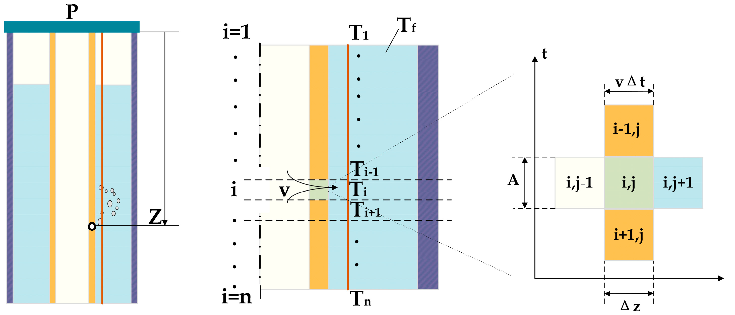
2.1. Mathematical Model

As the salt cavern gas storage is buried thousands of meters underground, there is a large temperature gap between the fluid in the wellbore and the formation environment, resulting in a rapid increase in the fluid temperature and annulus pressure in the enclosed space of casing annulus in each layer during the injection and production process [25]. In particular, the fluid in the annulus between the string and casing is affected by the high-temperature formation environment, which disturbs the stability of the wellbore temperature field and forms additional radial unsteady heat transfer in the limited confined space. The physical model of the string leakage process is shown in Figure 1. In the process of gas injection and production, the gas escapes from the leakage port into the annular fluid of the pipe string and casing, and the primary forms of heat flow include convective heat transfer between the gas and the annular fluid, heat conduction between the pipe string and the annular fluid, the Joule–Johnson effect caused by the gas flow, and the internal coupling of these forms of heat transfer [13]. Figure 2 illustrates the flow and heat transfer characteristics of the leakage port of the string, and the string can be divided into three parts: the gas in the injection–production pipe string, the injection–production pipe string, and the annulus fluid between the pipe string and casing.

Before building the prediction model in this paper, the following assumptions need to be made:

(1)

The temperature of the pipe column is symmetrical along the center line of the pipe column, and the pipe column is isotropic;

(2)

There is only one case of string leakage in the casing;

(3)

The annulus between the pipe string and the casing is sealed;

(4)

The thermal physical properties of each material in the wellbore remain unchanged;

(5)

No consideration is given to changes in borehole structure.

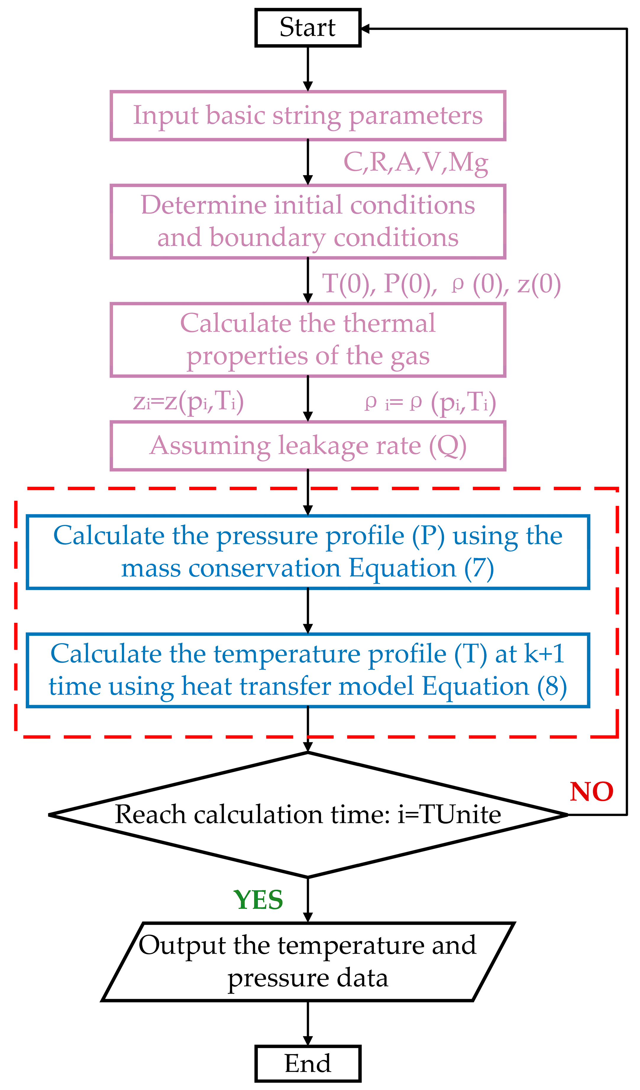
For the fluid in the string, there is a coupling effect between the fluid’s pressure, temperature, flow rate, and density [26]. Assume a compressible fluid in the tubing. When there is a leak in the wellbore, the fluid flow variable will change with time. According to gas flow characteristics before equilibrium, it belongs to unsteady and nonuniform flow. Because the fluid flowing out of the leakage aperture at the instantaneous moment still conforms to the energy conservation law, the inconsistent term is equal to the sum of the diffusion and source terms. Since the external heat transfer to the wellbore can be ignored in the case of wellbore micro-leakage, the source term can be omitted, and the energy equation can be established to obtain the following:

$$\rho A\Delta \mathrm{z}{\left.\left(U+\frac{v^2}{2}\right)\right|}_i^{{}_{t+△t}}-\rho A\Delta \mathrm{z}{\left.\left(U+\frac{v^2}{2}\right)\right|}_i^{{}_t}=\rho Av\Delta t{\left.\left(H+\frac{v^2}{2}\right)\right|}_i^{{}_{j+1}}-\rho Av\Delta t{\left.\left(H+\frac{v^2}{2}\right)\right|}_i^{{}_j}$$

(1)

where ρ is the fluid density, kg/m³; A is the leakage port area, m²; Δz is a micro-expression of the length of leakage path from the pipe column to the annulus; U is the internal energy of a molar gas at every moment, J/kg; v is the fluid leakage rate, m²/s; t is for time, s; Δt is the increment of time, s; and H is the energy carried by the fluid, J/kg. As shown in Figure 2, calibrate the wellbore axial spatial discretization through i (i = 0, 1, 2… n); calibrate the wellbore axial spatial discretization through j (j = 0, 1, 2… n).

Divide AΔzΔt for both sides of the equation:

$$\frac{\rho (U+\frac{v^2}{2})\left|\begin{array}{l}\\ t+△t\end{array}\right.-\rho (U+\frac{v^2}{2})\left|\begin{array}{l}\\ t\end{array}\right.}{△t}=\frac{v\rho (H+\frac{v^2}{2})\left|\begin{array}{l}\\ j+1\end{array}\right.-v\rho (H+\frac{v^2}{2})\left|\begin{array}{l}\\ j\end{array}\right.}{△z}$$

(2)

Take the partial derivative of both sides of the equation:

$$\frac{\partial \left[\rho (U+\frac{v^2}{2})\right]}{\partial t}=\frac{\partial \left[\rho v(H+\frac{v^2}{2})\right]}{\partial \mathrm{z}}$$

(3)

According to the first law of thermodynamics,

$$U=H-\frac{p}{\rho }$$

(4)

Substitute Formula (4) into Formula (3):

$$\begin{array}{l}\rho \frac{\partial H}{\partial t}+H\frac{\partial \rho }{\partial t}-\frac{\partial p}{\partial t}+\frac{v^2}{2}\frac{\partial \rho }{\partial t}+\rho v\frac{\partial v}{\partial t}\\ =vH\frac{\partial \rho }{\partial z}+\rho H\frac{\partial v}{\partial z}+\rho v\frac{\partial H}{\partial z}+\frac{v^3}{2}\frac{\partial \rho }{\partial z}+\frac{3\rho v^2}{2}\frac{\partial v}{\partial z}\end{array}$$

(5)

The phenomenon that the temperature of a gas changes after irreversible adiabatic expansion when it passes through a porous medium is called the Joule–Thomson effect. The total derivative of enthalpy can be derived from thermodynamic equilibrium relations. For the gas phase, the total derivative of enthalpy can be obtained via the thermodynamic equilibrium as shown in Equation (6):

$$\left\{\begin{array}{l}dH=C_{v,g}dT-{\mu }_{jT}{C}_{v,g}d\rho \\ \frac{\partial H}{\partial t}=C_{v,g}\frac{\partial T_f}{\partial t}-{\mu }_{jT}{C}_{v,g}\frac{\partial p}{\partial t}\\ \nabla H=C_{v,g}\nabla T_f-{\mu }_{jT}{C}_{v,g}\nabla p\end{array}\right.$$

(6)

where p is fluid pressure, Pa; μ_jT is the Joule–Thomson effect coefficient, K/Pa; C_v,g is the specific heat capacity of the fluid, J/(kg∙°C); T is the temperature of the leakage point, °C; and T_f is the temperature of pore fluid, °C.

By substituting Formula (6) into Formula (5), the fluid energy equation in its final form can be obtained:

$$\begin{array}{l}\rho C_{v,g}\frac{\partial T_f}{\partial t}-(\rho {\mu }_{jT}{C}_{v,g}+1)\frac{\partial p}{\partial t}+(C_{v,g}T+\frac{v^2}{2})\frac{\partial \rho }{\partial t}+\rho v\frac{\partial v}{\partial t}\\ =\rho v{C}_{v,g}\frac{\partial T_f}{\partial z}-\rho v{\mu }_{jT}{C}_{v,g}\frac{\partial p}{\partial z}+(v{C}_{v,g}T+\frac{v^3}{2})\frac{\partial \rho }{\partial z}+(\rho C_{v,g}T+\frac{3\rho v^2}{2})\frac{\partial v}{\partial z}\end{array}$$

(7)

2.2. Model Solving

The energy conservation, Equation (7), is solved numerically using the finite difference method, and the grid of the prediction model is first discretized. In this paper, the heterogeneous nodes of the prediction model are established according to the fluid in the pipe, the pipe, and the annulus fluid. For column axial space discretization I (i = 0, 1, 2… n) calibration and column radial space discretization j (0, 1, 2,… M) calibration, the node is represented by (i, j). The discrete time is calculated using n (n = 0, 1, 2… k). For calibration, Δt is a uniform time step. This prediction model considers the temperature, pressure, density, and velocity as variables and discretizes Formula (7) to obtain Formula (8), which represents the pore temperature value at the next time. The norehole unit division is shown in Figure 3:

$$\begin{array}{l}\rho C_{v,g}\frac{{T_f}^{k+1}-{T_f}^k}{\Delta t}-(\rho {\mu }_{jT}{C}_{v,g}+1)\frac{p^{k+1}-p^k}{\Delta t}+(C_{v,g}T+\frac{v^2}{2})\frac{{\rho }^{k+1}-{\rho }^k}{\Delta t}\\ +\rho v\frac{v^{k+1}-v^k}{\Delta t}=\rho v{C}_{v,g}\frac{T_f^{k+1}-T_f^k}{\Delta \mathrm{z}}-\rho v{\mu }_{jT}{C}_{v,g}\frac{p^{k+1}-p^k}{\Delta z}\\ +(v{C}_{v,g}T+\frac{v^3}{2})\frac{{\rho }^{k+1}-{\rho }^k}{\Delta z}+(\rho C_{v,g}T+\frac{3\rho v^2}{2})\frac{v^{k+1}-v^k}{\Delta z}\end{array}$$

(8)

To realize the coupling solution of fluid–string–annulus fluid, it is necessary not only to adopt the above fully implicit numerical discretization method but also to realize the simultaneous solution of the above equation under the same time step. The specific solution flow chart is shown in the figure below. The whole calculation process consists of two layers of iteration: the iterative solution of the pressure field and the iterative solution of the temperature field. Figure 4 is a detailed flowchart of the main program. The specific steps are as follows:

(1)

Input the initial temperature and pressure distribution of the inner and outer tubes;

(2)

Calculate the thermal physical property parameters of the gas according to the temperature and pressure field distribution calculated at time k or the last iteration;

(3)

Assume the leakage rate of pipe leakage port Q at time k;

(4)

The mass conservation equation is used to solve the pressure field distribution at k + 1 moment;

(5)

The fluid–column–annulus heat transfer model established in this paper is used to solve the temperature field distribution at k + 1;

(6)

Determine whether the temperature field distribution meets the convergence condition, and, if it does not, jump back to step (2);

(7)

Perform the k + 2 moment solution until the solution time is complete.

The solution process is as follows:

Figure 4. Detailed flow chart of the main program.

Figure 4. Detailed flow chart of the main program.

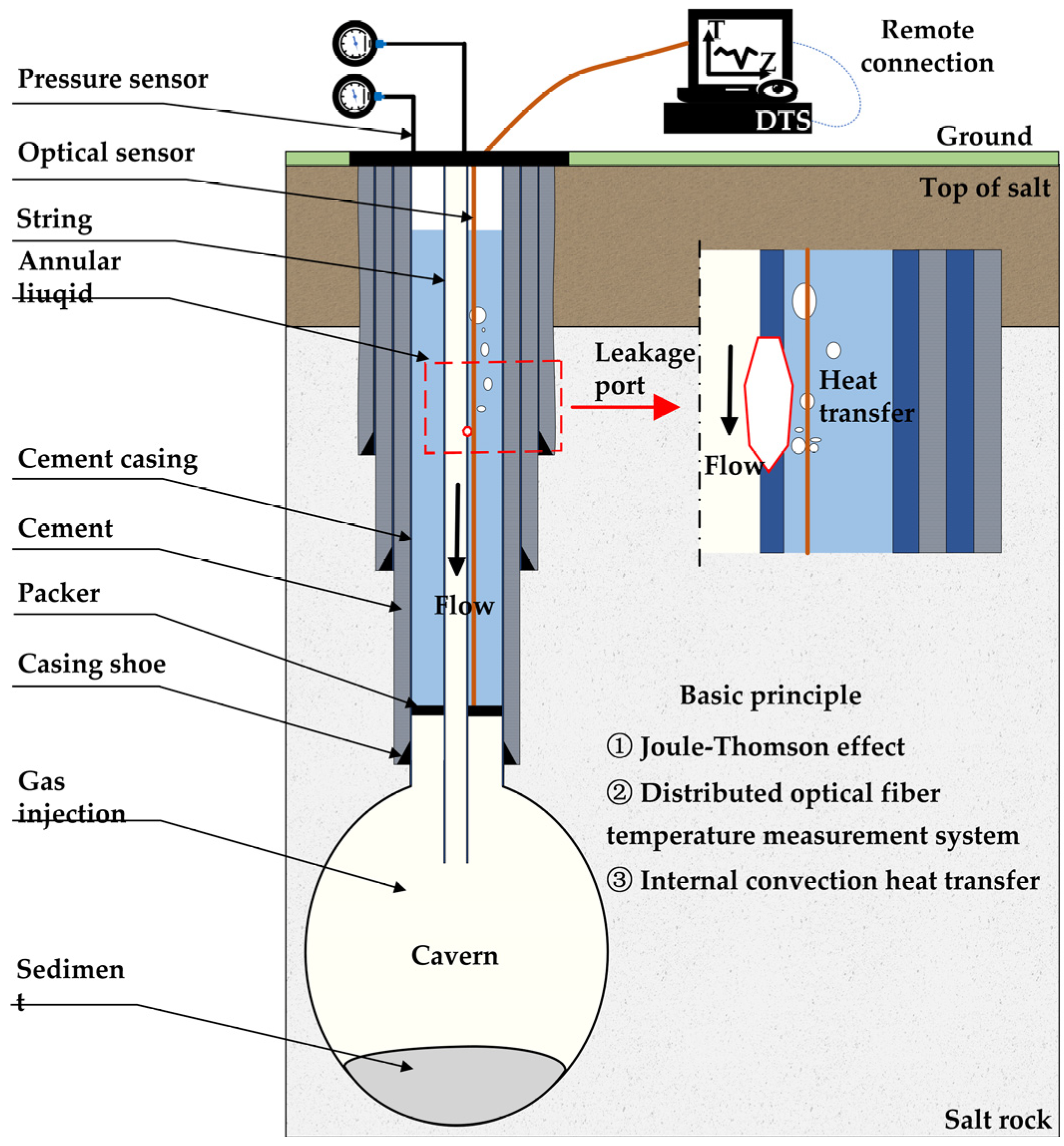
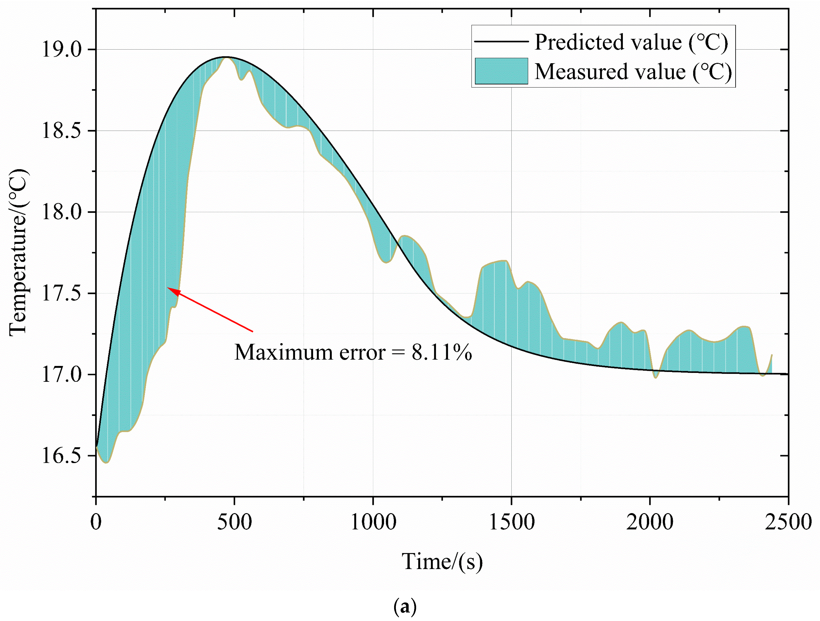
3. Experimental Verification

The second research work proposes a method and mathematical model for calculating the leakage rate of leakage ports in a string based on the temperature field. This section will verify the model by combining the DTS system and simulated wellbore installation. As shown in Figure 5a, the research group designed and built a set of full-size wellbore leakage indoor simulation devices with a double-layer string structure in the preliminary research work. The wall thickness of 304 stainless steel inner and outer strings is 0.01 m, the stainless steel outer string diameter d_outer is 0.246 m, the stainless steel inner string diameter d_inner is 0.178 m, the inner and outer strings are concentric, and the total length of the inner and outer strings L is 3 m. The side wall of the stainless steel inner string is provided with a leakage port with a diameter d of 0.025 m. The housing is connected with multiple flanges to facilitate the installation and replacement of leakage holes. There is a support structure between the internal line and the outer casing to ensure the concentricity of the inner and outer strings. The position of the leakage port is arranged on the inner wall of the string, and the leakage point is provided. The leakage valve is installed in the corresponding outer casing position to change the opening size of the leakage hole. The temperature-sensing cable is arranged to seal the inner casing wall close to the leakage valve. DTS measurements are made using multi-mode optical fibers.

Table 1. Measurement specifications of DTS.

DTS	Index
Detection unit length (spatial resolution)	0.02 m
Positioning accuracy	±1 m
Measuring time	<30 s
Temperature resolution	0.1 °C
Sampling interval	0.02 m
Temperature variation accuracy	0.5 °C (2000 m)

summarizes the specifications of the DTS used. The spatial resolution is the minimum fiber distribution length required to characterize the DTS for accurate temperature measurement along the fiber length distribution. The high-spatial-resolution DTS equipment used in this paper can reach 0.02 m; the positioning accuracy is the maximum deviation between the measured length value of the optical fiber temperature measuring device and the measured value of the standard ruler, the positioning error value. The sampling interval is 0.02 m, depending on the accuracy of the hardware device. Figure 5b shows the temperature change curve along the optical fiber distance finally detected by the DTS. During the experiment, a 3 m long string can monitor about 150 temperature points, among which the lowest temperature point showing drastic fluctuations in the curve is regarded as the leakage point, that is, the location of the leakage port. For safety reasons, gas is injected through a nitrogen simulated gas reservoir, and annular protection fluid is affected through water. In the simulation test device, a nitrogen cylinder is used to fill high-purity nitrogen into the oil pipe to manufacture natural gas, and water is set outside the casing to cram into the annulus to affect the annular protection fluid. Plugs are formed at both ends of the pipe string combination to seal, and the pipe string combination is lifted off the ground and kept vertically placed during the experiment. During the investigation, the compressed gas enters the annulus from the leak hole of the inner tube string. The temperature signal generated by the gas leak is received by the flexible optical cable (temperature-measuring multi-mode fiber) installed on the wall of the inner tube string and transmitted to the signal demodulation instrument, which converts the optical signal into an electrical signal and transfers it to the monitoring system in the computer, showing the graph between the visual fiber distance on the wall of the inner tube string and the temperature.

Compressed nitrogen was selected as the experimental gas because the preparation of nitrogen is simple and safe. At the same time, the main factors that affect the temperature change characteristics of the pipe string after pipe leakage are the pressure difference between the string and casing and the size of the leakage hole. Gas properties have little effect on optical fiber monitoring. In the DTS monitoring string leak test, it is first necessary to ensure the tightness of the device. After 2~6 MPa nitrogen is injected into the inner pipe string and the pressure of the inner and outer tanks is observed to remain unchanged for a while, it is considered that the device is qualified for sealing. After the sealing test, the leakage hole parameters are set according to the test plan. The leak aperture is 25 mm, and the opening angle of the leak opening can be set to 180° (245.313 mm²) by changing the valve size. Then, open the gas injection valve to inject nitrogen into the inner string at a preset pressure and stop the nitrogen injection when the pressure in the internal string reaches a specific value. Nitrogen in the inner string can enter the annulus through the leak hole, increasing the annular pressure. When the tension between the inner tube string and the annulus at the leak point is equal, when the pressure balance is reached, a set of temperature data of the internal tube string is collected. After one experiment, perform the following steps:

(1)

Open the bolts and flanges on the wall of the jacket tube.

(2)

Release the pressure in the annulus.

(3)

Replace the leak holes of other sizes and leak points of different depths.

(4)

Repeat the above experiment process.

The basic principle of DTS positioning technology based on the micro-leakage monitoring of the injection–production pipe string is as follows: the gas on both sides of the pipe leakage port flows out at the same time, and the gas accumulation on both sides causes the heat release phenomenon, resulting in the temperature increase of the pipe string on both sides of the leak port. When the gas passes through the hole plug, it absorbs heat due to the rapid expansion in the pressure drop process. The Joule–Thomson effect results in a significantly lower peak temperature at the leakage port. Based on this feature, the position of the string leakage port can be observed. As shown in Figure 6a,b, the temperature and pressure data at this point of the pipe string were obtained through the leakage test. The leakage rates at different times were calculated using Formula (9), and Formula (10) was fitted. The change law of the annular pressure p (t) and pipe temperature with the leakage time t of the leakage port under the condition of local micro-leakage at the leakage port was calculated to calculate the leakage rate prediction at the leakage port of the injectional production pipe string. A comparison was made with the experimental simulation results, as shown in Figure 6c.

$$v=\frac{VM}{\rho ZRT}\frac{d{P}_A}{dt}$$

(9)

$$v=0.0022-0.000002t$$

(10)

where P_A is the wellhead annulus pressure, Pa; V is the annulus volume, m³; M is the molar mass of gas, kg/kmol; Z is the compression factor; and R is the molar gas constant, J/(mol∙K).

As shown in Figure 6a, due to leakage, nitrogen in the pipe column floods into the annulus liquid, bubbles are generated due to the pressure difference, bubble diffusion is dispersed, and, after hitting the optical cable, it breaks back and constantly releases heat. However, this behavior is intermittent, and the temperature curve shows that the measured value’s temperature curve is an uninterrupted fluctuating rise. However, the peak value of the predicted leakage point temperature change calculated via software simulation and the estimated weight of the actual device coincides with the curve shape, and the maximum error is 8.11%.

As shown in Figure 6b, due to nitrogen injection into the annulus liquid at the leakage port, bubbles formed by pressure difference will spread around and surge to the place with low pressure. The pressure gauge at the side of the device will monitor the pressure value of the entire annulus, and the pressure curve will show slight fluctuations and not smooth due to the continuous rupture of bubbles. However, on the whole, when the pressure difference is 2 MPa, the predicted value of the leakage point pressure change calculated via software simulation and the final stabilizing value measured by the actual device coincide with the curve shape, and the maximum error is 9.59%.

As shown in Figure 6c, the initial leakage rate is the largest, and the pressure difference gradually decreases with the leakage process. On the whole, the leakage rate of the leakage point decreases linearly with time. The temperature and pressure values of the leakage point at different times were obtained through the test, and the time interval was 1 s. The leakage rate values of the leakage point at other times were obtained by calculating the temperature and pressure data combined with Formula (9). The error between the fitting curve of the leakage rate and the actual value is less than 5%, indicating that the prediction model proposed in this paper can accurately predict the leakage rate of the leakage point of the pipe string.

4. Sensitivity Analysis

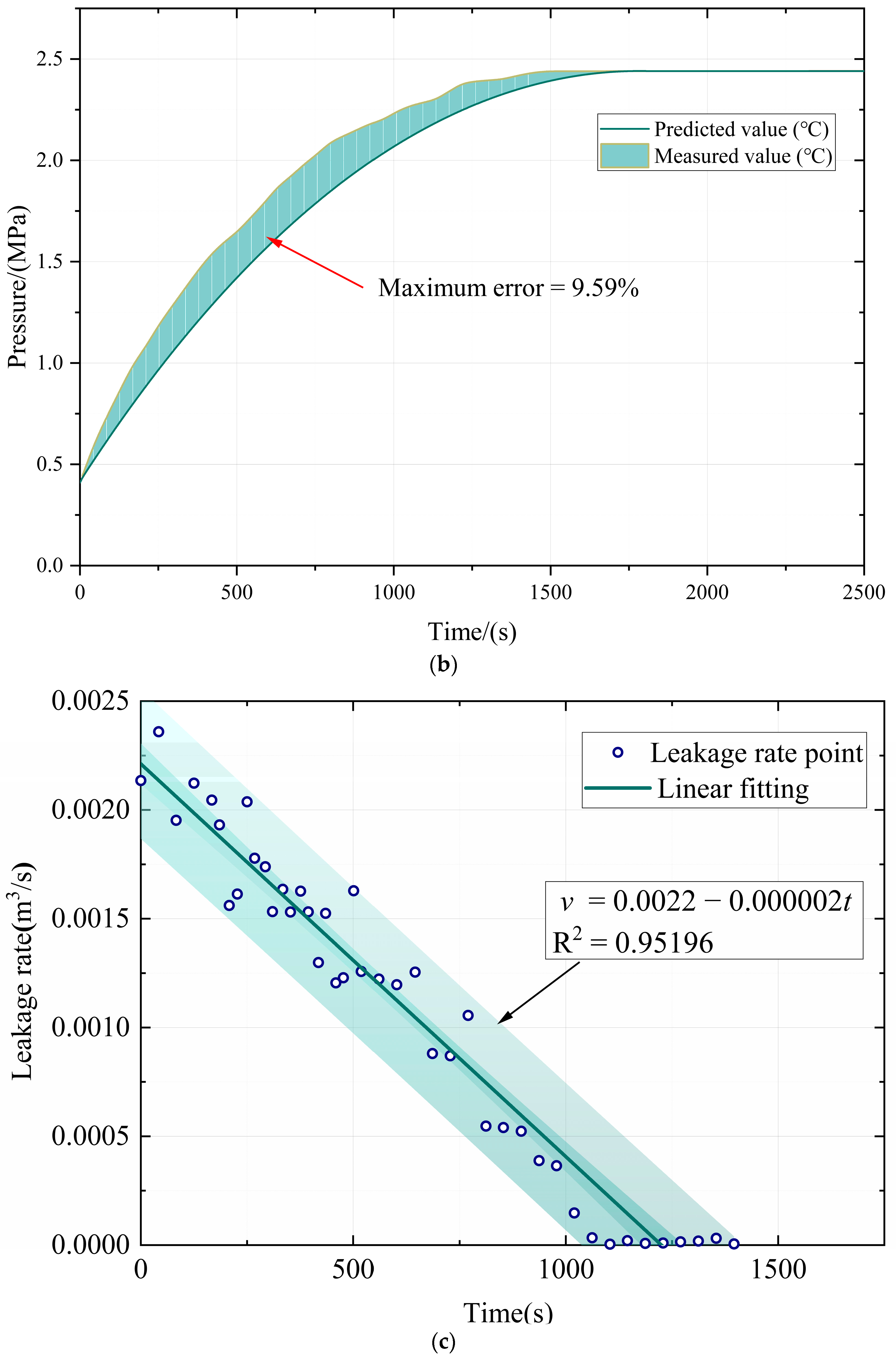
4.1. Leakage Rate

According to the test results of the wellbore tightness of an injection–production well in Jintan Salt Cave storage (

Table 2. Tightness test data of wellbores, including leakage location, average leakage rate, and interface displacement.

No.	Leakage Position (m)	Test Phase	Average Leakage Rate (m3/h)	Interface Displacement (m/h)
W1#	892.1~894.5	Phase 1	3.06	4.33
		Phase 2	0.71	4.11
W2#	893.2~895.4	Phase 1	0.10	0.40
		Phase 2	0.08	0.08
W3#	894.3~896.2	Phase 1	0.16	1.05
		Phase 2	0.03	0.42
W4#	903.2~904.3	Phase 1	0.12	0.05
		Phase 2	0.04	0.18
W5#	888.9~889.7	Phase 1	0.14	0.24
		Phase 2	0.09	0.03

) [27], the maximum leakage rate can reach 9.66 m³/h. In addition, the leakage rate of each wellbore in the second stage decreased significantly compared with that in the first stage: W1 decreased by 76.8%, and W3 decreased by 81.2%. The leakage rate decreases gradually with increases in time, which indicates that the leakage of the string is first rapid then slow and finally tends to be stable. Its basic parameters are shown in Table 2. To explore the change in temperature with time under different gas leakage rates, eight cases are explored in this section. The leakage rate values of the leakage point are 9.66 m³/h, 3.06 m³/h, 0.71 m³/h, 0.16 m³/h, 0.08 m³/h, 0.04 m³/h, 0.01 m³/h, and 0.001 m³/h. As shown in Figure 7, with the gradual decrease in the leakage rate, the fluctuation trend of the temperature curve at the leak point gradually weakens. When the leakage rate is 0.16 m³/h, the peak fluctuation of the temperature curve is less than 0.5 °C, while the leakage rate is reduced to 0.01 m³/h and 0.001 m³/h, and the temperature curve is close to the 0.16 m³/h curve. When the leakage rate is reduced to 0.16 m³/h, it is difficult for the DTS to accurately monitor when the temperature range is less than 0.5 °C.

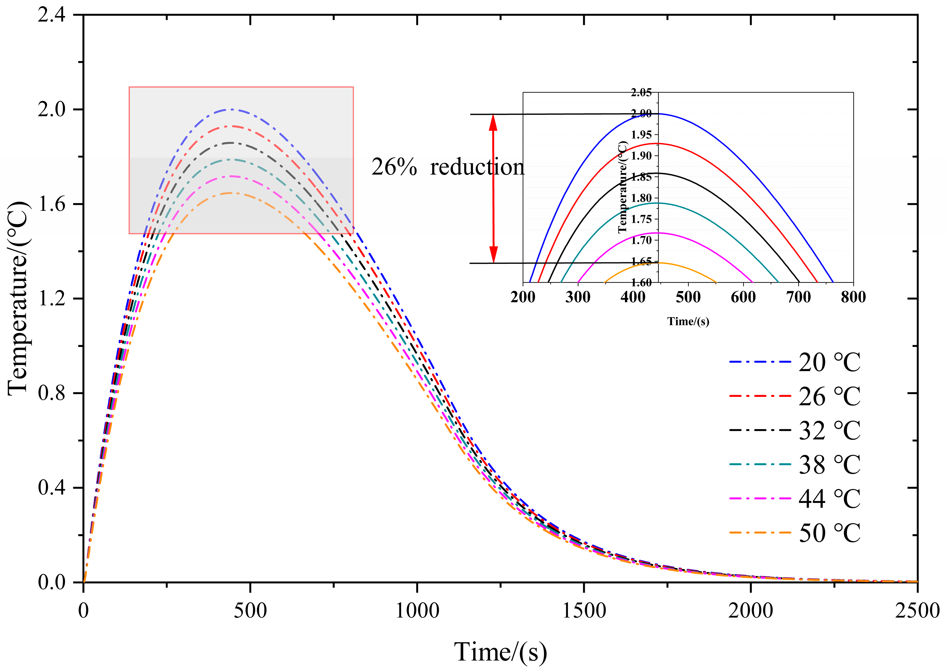
4.2. Ambient Temperature

The buried depth of salt cavern gas storage is generally 600–2000 m, and the string distribution is 0–1200 m. Due to the existence of a geothermal gradient, the influence of different ambient temperatures at different depths and gas densities on the evolution of the temperature field still needs to be supported by more detailed numerical simulation. In this section, sensitivity analysis under different ambient temperatures will be carried out to further reveal the temperature evolution law after gas leakage and provide theoretical support for further leakage prediction. Taking the basic parameters of Jintan injection production as an example (

Table 3. Summary of the basic parameters used for model performance.

Parameter	Value	Parameter	Value
Wellbore diameter	0.254 m	Ground temperature	20 °C
Gas recovery rate	35 m3/s	Geothermal gradient	0.03 °C/m
Gas production duration	8 d	Resting time	8 d
Initial gas storage pressure	16.5 MPa	The density of the surrounding rock	2650 kg/m3
Specific heat of gas	2347 J/(kg∙K)	Thermal conductivity of gas	0.15 W/(m∙K)
Specific heat of surrounding rock	999 J/(kg∙K)	Thermal conductivity of surrounding rock	2.09 W/(m∙K)

), the initial surface temperature is 20 °C, and the ground temperature gradient is 0.03 °C/m. The temperature variation rule of the well depth is 200 m (26 °C), 400 m (32 °C), 600 m (38 °C), 800 m (44 °C), and 1000 m (50 °C), and six conditions are studied under this rule. As can be seen from Figure 8, with the increase in depth and the growth in ambient temperature, the variation range of the temperature gradually decreases. In general, the variation trend of temperature curves at leakage points under different geothermal gradients is similar, and the temperature fluctuation difference between 0 and 1000 m depth is 0.45 °C, indicating that the geothermal gradient has a significant impact on the temperature monitoring of the DTS, which should be considered in the design of the DTS.

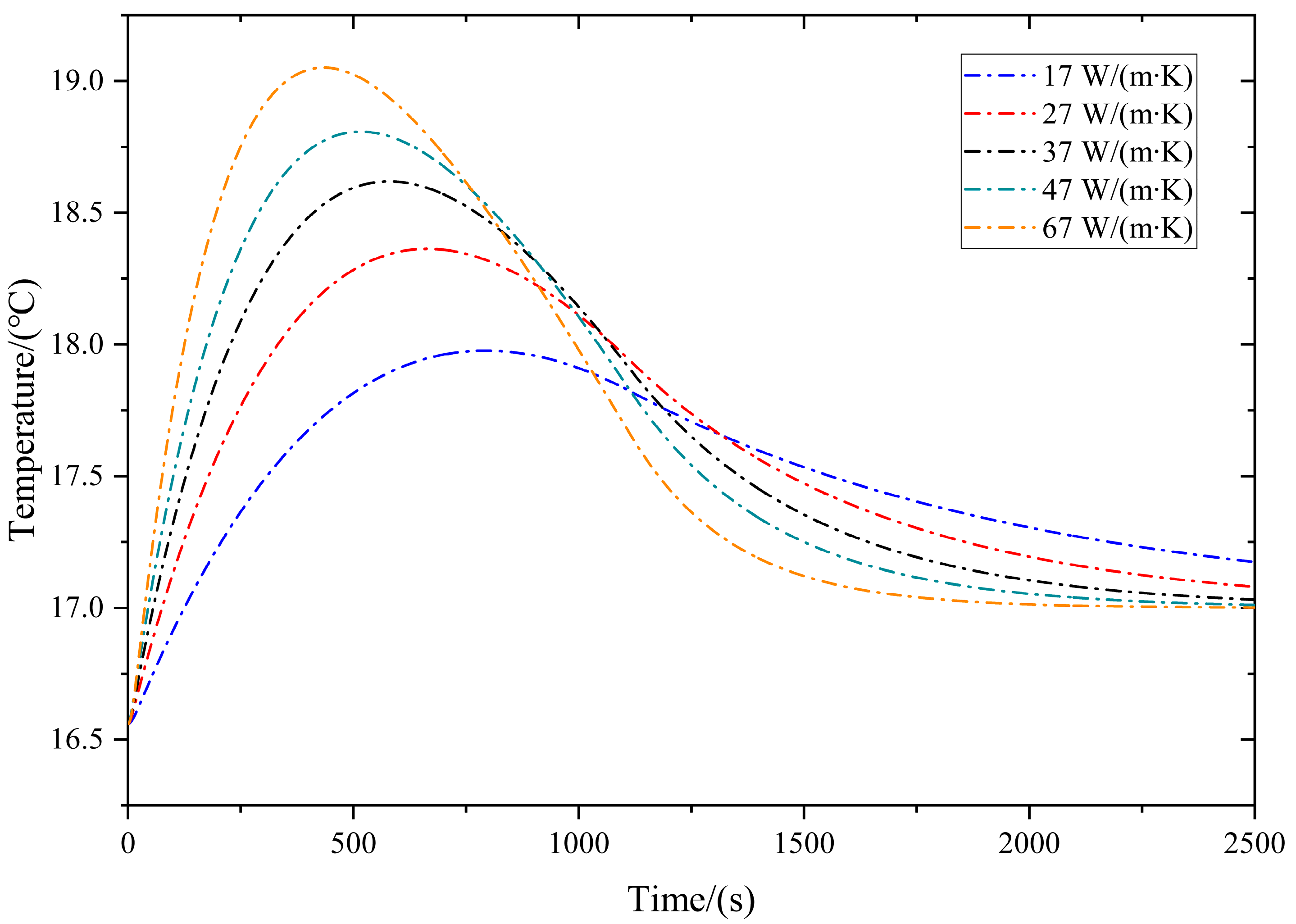
4.3. Heat Transfer Coefficient

The convective heat transfer coefficient is closely related to the physical characteristics, depth, and leakage rate of injection–production and annulus fluids. The convective heat transfer coefficient, meaning the convective heat transfer rate, is numerically equal to the convective heat transfer rate per unit heat transfer area under the unit temperature difference. The heat transfer coefficient of the string wall is closely related to the heat transfer coefficient of the gas and annulus liquid in the string, wall thickness, and fouling thermal resistance. This section will conduct sensitivity analysis under different convective heat transfer coefficients and column wall surface heat transfer coefficients and explore the influence law of different convective heat transfer coefficients and column wall heat surface transfer coefficients on the temperature change after gas leakage when the shape, depth, and leakage rate are unchanged. The values of the convective heat transfer coefficient were selected as 222 W/(m²∙K), 422 W/(m²∙K), 522 W/(m²∙K), and 822 W/(m²∙K). It can be seen from Figure 9 that the higher the convective heat transfer coefficient and the stronger the heat transfer capacity between the fluid and the solid, the more pronounced the temperature change. The column wall surface heat transfer coefficient refers to the ability of a string wall to transfer heat per unit area in unit time. The values of the string wall surface heat transfer coefficient are 17 W/(m·K), 27 W/(m·K), 37 W/(m·K), 47 W/(m·K), and 67 W/(m·K), respectively. It can be seen from Figure 10 that, with the increase in the wall heat transfer coefficient, the temperature range gradually increases, and the speed of rising to the peak point gradually increases. However, with the gradual decrease in the leakage rate, the temperature of the leak point with a significant wall heat transfer coefficient decreases faster, which indicates that DTS monitoring equipment is more suitable for the injection production string with a significant wall heat transfer coefficient, the string diameter is more extensive, and the wall thickness is thinner. This study will help analyze the feasibility of DTS monitoring string leaks.

5. Conclusions

In this paper, a new mathematical formula for predicting the gas leakage rate in an injection–production string of salt cavern gas storage using distributed temperature sensing technology (DTS) is presented, and the following conclusions are obtained:

• The formula for calculating the heat transfer at the leakage port under unsteady temperature conditions was established, and the quantitative relationship between the temperature difference and leakage rate was set by considering the Joule–Thomson effect. The predicted value of the gas leakage rate was obtained by inverting the temperature data of the string.
• A simulation test of leakage monitoring for the injection–production string of salt cavern gas storage was carried out. Combined with DTS monitoring technology, the measured temperature value of string leakage under pressure was obtained. By comparing the calculated value with the predicted value, the prediction of the leakage rate was realized, and the maximum error was less than 5%, which verified the accuracy of the mathematical model.
• The sensitivity of the leakage rate, ambient temperature, and related heat transfer coefficient was evaluated. The results showed that when the leakage rate value was reduced to 0.16 m³/h, it would be difficult to accurately monitor the DTS when the temperature change range was less than 0.5 °C; the ambient temperature significantly influences temperature monitoring, and the temperature fluctuation error at 20 to 50 °C is 26%. This influence factor should be considered when designing the DTS.

References

1. Yang, C.; Wang, T. Deep Underground Energy Storage: Aiming for Carbon Neutrality and Its Challenges. In Engineering; Elsevier: Amsterdam, The Netherlands, 2023. [Google Scholar]
2. Haldorsen, H.H. Invited Perspective: The Outlook for Energy: A View to 2040. J. Pet. Technol. 2015, 67, 14–19. [Google Scholar]
3. Yang, C.; Wang, T.; Chen, H. Theoretical and Technological Challenges of Deep Underground Energy Storage in China. Engineering 2022. [Google Scholar] [CrossRef]
4. Al-Shafi, M.; Massarweh, O.; Abushaikha, A.S.; Bicer, Y. A review on underground gas storage systems: Natural gas, hydrogen and carbon sequestration. Energy Rep. 2023, 9, 6251–6266. [Google Scholar] [CrossRef]
5. Zhang, Y.; Oldenburg, C.M.; Zhou, Q.; Pan, L.; Freifeld, B.M.; Jeanne, P.; Tribaldos, V.R.; Vasco, D.W. Advanced monitoring and simulation for underground gas storage risk management. J. Pet. Sci. Eng. 2022, 208, 109763. [Google Scholar] [CrossRef]
6. He, T.; Wang, T.; Wang, D.; Xie, D.; Dong, Z.; Zhang, H.; Ma, T.; Daemen, J. Integrity analysis of wellbores in the bedded salt cavern for energy storage. Energy 2023, 263, 125841. [Google Scholar] [CrossRef]
7. Evans, D.J. A review of underground fuel storage events and putting risk into perspective with other areas of the energy supply chain. Geol. Soc. Lond. Spec. Publ. 2009, 313, 173–216. [Google Scholar] [CrossRef]
8. Li, H.Z.; Saint-Vincent, P.M.B.; Mundia-Howe, M.; Pekney, N.J. A national estimate of U.S. underground natural gas storage incident emissions. Environ. Res. Lett. 2022, 17, 084013. [Google Scholar] [CrossRef]
9. Zhao, L.; Yan, Y.; Wang, P.; Yan, X. A risk analysis model for underground gas storage well integrity failure (Article). J. Loss Prev. Process Ind. 2019, 62, 103951. [Google Scholar] [CrossRef]
10. Jayawickrema, U.M.N.; Herath, H.; Hettiarachchi, N.; Sooriyaarachchi, H.; Epaarachchi, J. Fibre-optic sensor and deep learning-based structural health monitoring systems for civil structures: A review. Measurement 2022, 199, 111543. [Google Scholar] [CrossRef]
11. Wang, J.; Han, Y.; Cao, Z.; Xu, X.; Zhang, J.; Xiao, F. Applications of optical fiber sensor in pavement Engineering: A review. Constr. Build. Mater. 2023, 400, 132713. [Google Scholar] [CrossRef]
12. Sun, Y.; Xue, Z.; Hashimoto, T. Fiber optic distributed sensing technology for real-time monitoring water jet tests: Implications for wellbore integrity diagnostics. J. Nat. Gas Sci. Eng. 2018, 58, 241–250. [Google Scholar] [CrossRef]
13. Tabjula, J.L.; Wei, C.; Sharma, J.; Santos, O.L.; Chen, Y.; Kunju, M.; Almeida, M.; Upchurch, E.R.; Samdani, G.A.; Moganaradjou, Y.; et al. Well-scale experimental and numerical modeling studies of gas bullheading using fiber-optic DAS and DTS. Geoenergy Sci. Eng. 2023, 225, 211662. [Google Scholar] [CrossRef]
14. Leone, M. (INVITED)Advances in fiber optic sensors for soil moisture monitoring: A review. Results Opt. 2022, 7, 100213. [Google Scholar] [CrossRef]
15. Liu, Y.H.; Ai, G. Numerical Study on the Heat Transfer in the Leakage of Pressure Vessels Considering the Joule-Thomson Cooling Effect. Procedia Eng. 2015, 130, 232–249. [Google Scholar] [CrossRef]
16. Nuñez-Lopez, V.; Muñoz-Torres, J.; Zeidouni, M. Temperature monitoring using Distributed Temperature Sensing (DTS) technology. Energy Procedia 2014, 63, 3984–3991. [Google Scholar] [CrossRef]
17. Tarmoom, I.; Thabet, H.B.; Samad, S.; Chishti, K.; Hussain, A.; Arafat, M. A Comprehensive Approach to Well-Integrity Management in Adma-Opco. In SPE Middle East Oil and Gas Show and Conference; SPE: Kuala Lumpur, Malaysia, 2007. [Google Scholar]
18. Wu, S.; Zhang, L.; Fan, J.; Zhang, X.; Zhou, Y.; Wang, D. Prediction analysis of downhole tubing leakage location for offshore gas production wells. Measurement 2018, 127, 546–553. [Google Scholar] [CrossRef]
19. Kabir, C.; Izgec, B.; Hasan, A.; Wang, X. Computing flow profiles and total flow rate with temperature surveys in gas wells. J. Nat. Gas Sci. Eng. 2012, 4, 1–7. [Google Scholar] [CrossRef]
20. Alan, C.; Cinar, M. Interpretation of temperature transient data from coupled reservoir and wellbore model for single phase fluids. J. Pet. Sci. Eng. 2022, 209, 109913. [Google Scholar] [CrossRef]
21. Pan, L.; Oldenburg, C.M.; Wu, Y.-S.; Pruess, K. Wellbore flow model for carbon dioxide and brine. Energy Procedia 2009, 1, 71–78. [Google Scholar] [CrossRef]
22. Wiese, B. Thermodynamics and heat transfer in a CO2 injection well using distributed temperature sensing (DTS) and pressure data. Int. J. Greenh. Gas Control 2014, 21, 232–242. [Google Scholar] [CrossRef]
23. Soliman, E.M.; Lee, D.; Stormont, J.C.; Taha, M.M.R. New mathematical formulations for accurate estimate of nitrogen leakage rate using distributed temperature sensing in Mechanical Integrity Tests. J. Pet. Sci. Eng. 2022, 215, 110710. [Google Scholar] [CrossRef]
24. Trudel, E.; Frigaard, I.A. Stochastic modelling of wellbore leakage in British Columbia. J. Pet. Sci. Eng. 2023, 220, 111199. [Google Scholar] [CrossRef]
25. Wu, S.; Zhang, L.; Fan, J.; Zhang, X.; Liu, D.; Wang, D. A leakage diagnosis testing model for gas wells with sustained casing pressure from offshore platform. J. Nat. Gas Sci. Eng. 2018, 55, 276–287. [Google Scholar] [CrossRef]
26. Hasan, A.R.; Kabir, C.S. Wellbore heat-transfer modeling and applications (Review). J. Pet. Sci. Eng. 2012, 86–87, 127–136. [Google Scholar] [CrossRef]
27. Wang, T.; Chai, G.; Cen, X.; Yang, J.; Daemen, J. Safe distance between debrining tubing inlet and sediment in a gas storage salt cavern. J. Pet. Sci. Eng. 2021, 196, 107707. [Google Scholar] [CrossRef]
Figure 1. Schematic diagram of distributed temperature sensing (DTS) system used for leak monitoring of injection–production string of salt cavern gas storage.
Energies 16 06173 g001
Figure 2. Schematic diagram of two-dimensional pipe leakage diameter to heat transfer.
Energies 16 06173 g002
Figure 3. Discrete model of pipe leakage heat transfer.
Energies 16 06173 g003
Figure 5. Schematic diagram of the test device. (a) The connection of the test device and the expression of the position of the leakage port; (b) Temperature changes along the length of the cable and the specific display of the leak point location monitored by DTS.
Energies 16 06173 g005aEnergies 16 06173 g005b
Figure 6. Comparison between the predicted value and the measured value when the leakage opening is 180°, and the internal and external pressure difference is 2 MPa: (a) Time–annular pressure curve at the leak point; (b) description of time–temperature curve at the leak point; (c) description of time–leakage rate curve at the leak point.
Energies 16 06173 g006aEnergies 16 06173 g006b
Figure 7. Temperature change with time at different leakage rates.
Energies 16 06173 g007
Figure 8. Temperature fluctuation range of leakage points at different depths with time.
Energies 16 06173 g008
Figure 9. Variation in temperature fluctuation range of leakage point with time under different convective heat transfer coefficients.
Energies 16 06173 g009
Figure 10. Temperature fluctuation range of leakage point under different string wall heat transfer coefficient changes with time.
Energies 16 06173 g010