Balancing Profit and Environmental Sustainability with Carbon Emissions Management and Industry 4.0 Technologies

Abstract

The environmental pollution issue in the textile industry has gained significant attention recently as one of the world’s most polluting industries. This paper aims to optimize product mixes for profit, tax, carbon, and resource efficiency. It employs mathematical models based on Activity-Based Costing (ABC) and the Theory of Constraints (TOC) to address carbon emissions, waste reuse, and energy recovery. Industry 4.0 technologies are integrated with real-time sensing and detection in production, and data are analyzed in the ERP system for optimal responses to production issues. The study explores different carbon emission cost models, including balancing environmental protection and green production with maximizing corporate profits. Additionally, a new environmentally friendly brick is proposed, combining cement with emitted coal slag to create a cost-effective and eco-friendly product.

1. Introduction

The traditional textile industry has long been known for being both labor-intensive and highly polluting [1]. Up to 8000 chemicals may be used to produce a single garment, from dyeing to final processing. The fast-fashion business model, with its short product life cycle, is causing ecological pressure, and its pollution level is second only to the petrochemical industry. To meet current fashion trends, the textile industry must adopt some level of diversity or customization in production [2,3,4]. Therefore, technological improvements in the manufacturing process have become necessary. In recent years, Industry 4.0 has gained popularity as a manufacturing trend for optimizing factories through advanced technology. This not only optimizes manufacturing processes [5] but also aids in data monitoring and maintenance to effectively control industrial pollution [6,7]. The first smart manufacturing demonstration of Industry 4.0 was at Hannover Messe 2011 in Germany [3]) and garnered attention [8,9]. Industry 4.0 relies on system components and sensors to collect data for analysis in the ERP system to promptly address production issues.

There is a lack of consensus on how to balance profit and environmental sustainability, and there are unanswered questions about how Industry 4.0 technologies can be used to reduce carbon emissions. The components and sensors in Industry 4.0 can facilitate waste recycling and carbon emission reduction. To fill the current literature gap, this paper aims to integrate Industry 4.0, ERP, ABC, TOC [5], and environmental concerns to enhance green production efficiency, while also considering carbon emissions, energy recovery, waste reuse, and profit maximization. The components and sensors in Industry 4.0 can facilitate waste recycling and carbon emission reduction.

This article is divided into seven parts: the research background, construction of a green production model under activity-based costing for a single period, analysis of the single-period model using Lingo 16.0, extension of the single-period model into a multi-phase model with time factors, optimal solution of the multi-period model using Lingo 16.0 with sensitivity analysis, and conclusion.

2. Research Background

2.1. Introduction to Industry 4.0

The world has experienced four industrial revolutions since the 18th century, each driven by major technological innovations. The first revolution began with the steam engine, followed by the second revolution with the invention of electricity. The third revolution emerged with the development of semiconductors, networks, and computers. Currently, the world is witnessing the beginning of the Fourth Industrial Revolution [10]. Industry 4.0 combines network systems, IoT, big data, and cloud computing to improve production efficiency. It means using automated robots, sensors, supply chains, and human–machine collaboration to optimize manufacturing for zero downtime, waiting, and maximum customization. Sensors on machines capture process data and monitor machine status to prevent wear and make timely replacements. Real-time machine status helps plan maintenance schedules to avoid unexpected downtime and optimize yield to reduce scrap loss, extend tool life, reduce tool cost, and increase productivity [11,12].

2.2. The Impact of Industry 4.0 on the Textile Industry

The textile industry is a major source of environmental pollution, particularly in terms of carbon emissions. As a result, there is an increasing awareness of the need for environmental protection and green products [5]. Moreover, the textile industry is now more focused on production processes to meet carbon emission standards and green product demands. However, due to the industry’s labor-intensive and complex manufacturing processes, as well as its long supply chain, small-batch customized production requires a smart factory [13], and the cyber–physical system (CPS) or virtual–real integration system is the most relevant for the textile industry and Industry 4.0. The CPS enables the textile machines to be more flexible and communicative and facilitates self-optimizing production and faster response to machine failures or repairs [14]. A review by Mahmood, Haider, et al. [15] suggests that policy interventions, such as environmental information transparency and government-business relations, can play a vital role in enhancing environmental sustainability in China.

2.3. Relationship between ERP, TOC, ABC, and Industry 4.0

Activity-based costing (ABC) accurately calculates product costs, while TOC maximizes profits for some companies. Industry 4.0 sensors collect machine data [16,17,18], which are analyzed using big data [19] and cloud computing in the ERP system. Afterward, the manufacturing production system (MES) is used to issue production instructions, and automated technical assistance improves the production process. These four concepts and their relationship are displayed in Figure 1.

3. Research Design and Methods

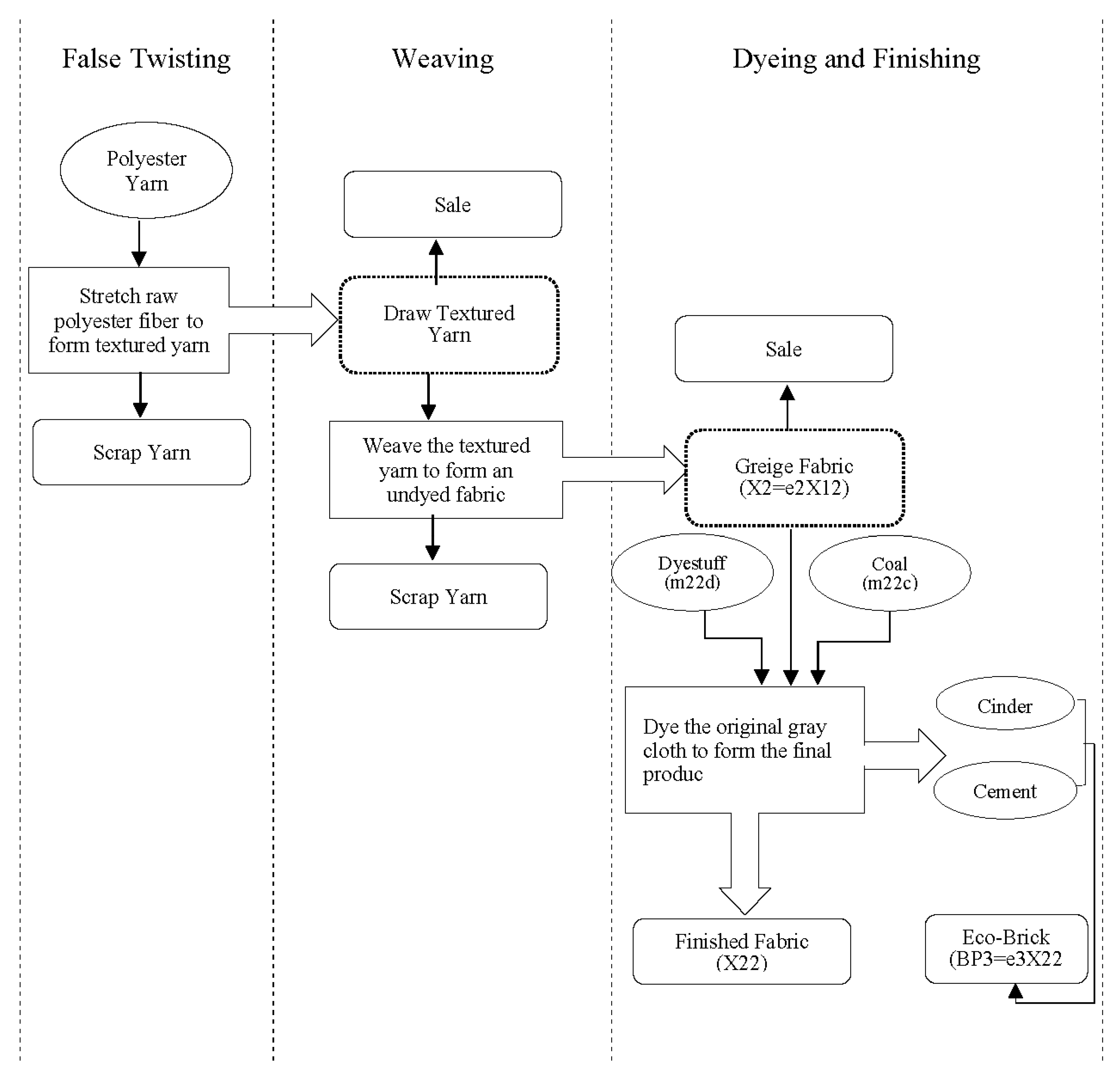
3.1. The Production Process of a Typical Textile Company

The textile industry is traditionally labor-intensive [13], with multiple processes required to produce finished products. These include false twisting, weaving, dyeing, and finishing. In the traditional textile industry, the finished product is obtained through false twisting, weaving, and dyeing/finishing. False twisting is used to stretch raw polyester fiber to form textured yarn. Weaving is used to weave the textured yarn to form an undyed fabric, while dyeing/finishing is used to dye the original gray cloth to form the final product. However, the dyeing process usually requires high heat generated through coal, which damages the environment. To address this, an environmentally friendly brick can be produced by combining cement and discharged cinder, which has a light texture and good permeability. This new product can help save raw material costs while also benefiting the environment.

3.2. Process Assumptions

This paper applies Industry 4.0’s decision-making model to vertically integrate textile production. In the first false-twisting process, each unit of processed polyester fiber raw material will produce ${\mathrm{e}}_1$ unit of textured yarn after false-twisting stretching and then subsequently produce a $1-{\mathrm{e}}_1$ unit of waste fabric. The produced textured yarn can be sold or further entered into the next weaving process, and the waste cloth can also be sold at a lower price. After the second weaving process, each unit of textured yarn can produce ${\mathrm{e}}_2$ units of original gray cloth and then produce ${1-\mathrm{e}}_2$ units of waste cloth, and the original gray cloth can still be sold or further processed for the next dyeing-and-finishing process. After dyeing and finishing, the finished fabric can be produced. Assumptions for the decision-making model of green production in Industry 4.0 include the following: (1) Divide all handling activities into single-batch handling. (2) This model does not involve expansion, and outsourcing (3) can increase the working hours of labor through overtime working hours to meet the higher wage rates stipulated by the government. (4) Carbon dioxide emission costs vary based on emission levels and tax rates, with certain models factoring in carbon weight.

3.3. Single-Period Objective Function

The structure of the green production planning model under ABC and Industry 4.0 is shown in the main equation. The carbon tax component is analyzed in eight cases in this paper, while the other components of the model, such as the main product income, by-product income, raw material cost, direct labor cost, heat and water recovery, and fixed cost, remain unchanged. This section introduces the relevant coefficients, while the models for changing the carbon tax are discussed in Section 3.4.

The objective function for maximum profit and the model’s variables can be defined as follows:

Maximum profit = main product income + by-product income − raw material cost − direct labor cost − carbon tax + heat and water recovery − fixed cost

$$\begin{gathered} \pi =\left[P_1{X}_{11}+P_2{X}_{21}+P_3{X}_{22}+{\beta }_1\left(1-e_1\right)M+{\beta }_2\left(1-e_2\right)X_{12}+{\beta }_3{e}_3{X}_{22}\right] \\ -\left[\left(C_{1}M+C_2{m}_{22d}\right)+\left(C_3{m}_{22c}+C_4{m}_{22m}\right)\right] \\ -\left[L_0+{\eta }_1{r}_{ot}\left(Q_1-G_0\right)\right]-\mathrm{c}\mathrm{a}\mathrm{r}\mathrm{b}\mathrm{o}\mathrm{n} \mathrm{t}\mathrm{a}\mathrm{x}+\left({\mathrm{C}}_5{\mathrm{R}\mathrm{E}}_{\mathrm{h}}+{\mathrm{C}}_6{\mathrm{R}\mathrm{E}}_{\mathrm{w}}\right)-\mathrm{F} \end{gathered}$$

(1)

In the above equation, we have the following:

${\mathrm{P}}_{\mathrm{i}}$	The selling price per unit of the product;
${\mathrm{X}}_{11}$	Textured Yarn Sales Quantity;
${\mathrm{X}}_{12}$	The amount of textured yarn that will enter the weaving process;
${\mathrm{X}}_{21}$	Sales volume of raw gray cloth;
${\mathrm{X}}_{22}$	Sales volume of finished cloth;
${\mathsf{\beta }}_{\mathrm{i}}$	By-product sales;
${\mathrm{e}}_1$	Input–output relationship coefficient in false twisting process;
${\mathrm{e}}_2$	Input–output relationship coefficient in weaving process;
${\mathrm{e}}_3$	The input–output relationship coefficient of manufacturing environmentally friendly bricks;
${\mathrm{c}}_1,{\mathrm{c}}_2,{\mathrm{c}}_3,{\mathrm{c}}_4$	$\mathrm{Unit} \mathrm{material} \cos \mathrm{t} \mathrm{of} \mathrm{M},{\mathrm{m}}_{22\mathrm{d}},{\mathrm{m}}_{22\mathrm{c}},{\mathrm{m}}_{22\mathrm{m}}$;
${\mathrm{c}}_5,{\mathrm{c}}_6$	Cost of heat and water saved per unit of recycling;
$\mathrm{M}$	The quantity of raw material polyester fiber;
${\mathrm{m}}_{22\mathrm{d}}$	Quantity of dye raw materials;
${\mathrm{m}}_{22\mathrm{c}}$	The amount of cinder produced;
${\mathrm{m}}_{22\mathrm{m}}$	Amount of cement;
${\mathrm{L}}_0$	Direct labor costs for regular hours;
${\mathsf{\eta }}_0,{\mathsf{\eta }}_1$	This is a dummy variable of 0 and 1;
${\mathrm{r}}_{\mathrm{o}\mathrm{t}}$	Wage rate for direct labor in case of overtime;
${\mathrm{Q}}_1$	Overtime;
${\mathrm{G}}_0$	Working Hours Limits for Regular Working Hours;
${\mathrm{R}\mathrm{E}}_{\mathrm{h}},{\mathrm{R}\mathrm{E}}_{\mathrm{w}}$	Heat and water recovery in green energy;
$\mathrm{F}$	Fixed cost.

3.3.1. Unit Direct Labor Cost Function

The model assumes that labor can work overtime to process materials and products, with a piecewise linear total cost function for direct labor. Figure 2 shows that the normal direct working hours are ${\mathrm{G}}_0$, which can be extended to ${\mathrm{G}}_1$ at an increased cost of ${\mathrm{L}}_0$, ${\mathrm{L}}_0+{\mathrm{r}}_{\mathrm{o}\mathrm{t}}{\mathrm{G}}_1$. Direct labor includes time for changing materials and resetting batch programs in dyeing, as well as manual labor for transferring products between processes. The formula and associated constraints for direct labor are given below:

$$\begin{gathered} l_{1}M+l_2{X}_{12}+l_3{X}_{22}+{\mu }_{01}{B}_{01}+{\mu }_{12}{B}_{12}+{\mu }_{10}{B}_{10} \\ +{\mu }_{23}{B}_{23}+{\mu }_{20}{B}_{20}+{\mu }_{30}{B}_{30}+\omega BS=Q_0+Q_1 \end{gathered}$$

(2)

$$0\le Q_0\le {\eta }_O{G}_0$$

(3)

$${\eta }_1{G}_0\le Q_1\le {\eta }_1{G}_1$$

(4)

$${\eta }_0{+\eta }_1=1$$

(5)

In the above constraints, we have the following:

${\mathrm{l}}_1$	Direct labor time required to move M;
${\mathrm{l}}_2$	Direct labor time required to move ${\mathrm{X}}_{12}$;
${\mathrm{l}}_3$	Direct labor time required to move ${\mathrm{X}}_{22}$;
${\mathsf{\mu }}_{\mathrm{s},\mathrm{e}}$	Direct labor time per batch activity from start to finish;
${\mathrm{B}}_{\mathrm{s},\mathrm{e}}$	The number of shipments per batch activity from start to finish;
$\mathsf{\omega }$	Setup time per batch of direct labor;
$\mathrm{B}\mathrm{S}$	Set the quantity of products in the batch activity;
${\mathrm{Q}}_0$	Direct labor hours in normal working hours;
${\mathrm{Q}}_1$	Overtime hours;
${\mathrm{G}}_0$	Limits on normal direct labor hours;
${\mathrm{G}}_1$	Direct labor hour limits for overtime;
${\mathsf{\eta }}_0,{\mathsf{\eta }}_1$	This is a dummy variable of 0 and 1.

3.3.2. Batch Cost Transfer Function

This model considers batch activities in the production process, including material and product handling from start to finish, as well as dye setting during the dyeing-and-finishing process. Each finished in-process product is then shipped back to the factory for sale. The associated formulas and constraints are presented below:

$$M\le {\sigma }_{01}{B}_{01}$$

(6)

$$X_{12}\le {\sigma }_{12}{B}_{12}$$

(7)

$$X_{11}+\left(1-e_1\right)M\le {\sigma }_{10}{B}_{10}$$

(8)

$$X_{22}\le {\sigma }_{23}{B}_{23}$$

(9)

$$X_{21}+\left(1-e_2\right)X_{12}\le {\sigma }_{20}{B}_{20}$$

(10)

$$X_{22}+e_3{X}_{22}\le {\sigma }_{30}{B}_{30}$$

(11)

$$X_{22}\le \lambda BS$$

(12)

In the above associated formulas and constraints, we have the following:

${\mathsf{\sigma }}_{\mathrm{s},\mathrm{e}}$—The number of moves per batch activity from start to finish;

$\mathsf{\Lambda }$—Set quantity for batch activity.

3.3.3. Heat Energy and Water Energy Recovery Function

The textile industry heavily relies on heat for the dyeing-and-finishing process, usually generated through coal-powered steam boilers, high-temperature air heat transfer, and heat recovery from exhaust gases. Additionally, the industry is also known to consume a significant amount of water [5] (Schoeberl, Brik et al., 2005), making water recycling an essential issue [20] (Lopez, Ricco, et al., 1999). The dyeing-and-finishing process [21] (Chequer, de Oliveira, et al., 2013), in particular, requires the most heat and water, with varying resource recovery rates. The costs for recovering heat and water are denoted as ${\mathrm{C}}_5{\mathrm{R}\mathrm{E}}_{\mathrm{h}} \mathrm{a}\mathrm{n}\mathrm{d} {\mathrm{C}}_6{\mathrm{R}\mathrm{E}}_{\mathrm{w}}$, and their related constraints are as follows:

$${\mathrm{R}\mathrm{E}}_{\mathrm{h}}={\mathsf{\rho }}_1\times {\mathrm{X}}_{22}$$

(13)

$${\mathrm{R}\mathrm{E}}_{\mathrm{w}}={\mathsf{\rho }}_2\times {\mathrm{X}}_{22}$$

(14)

In the above constraints, we have the following:

${\mathsf{\rho }}_1$—Correlation coefficient between heat energy recovery and ${\mathrm{X}}_{22}$;

${\mathsf{\rho }}_2$—Correlation coefficient between water energy recovery and ${\mathrm{X}}_{22}$.

3.3.4. Input–Output Relationship Function

Material input may result in losses during the production process, leading to a difference between input and output quantities. Let ${\mathrm{X}}_{12}$ be the input quantity of deformed yarn, ${\mathrm{e}}_2{\mathrm{X}}_{12}$ be the output quantity of original gray cloth, and $\left(1-{\mathrm{e}}_2\right){\mathrm{X}}_{12}$ be the output quantity of waste cloth. Figure 3 is a flowchart that shows the different stages of textile manufacturing with variable symbols. The associated constraint formula is as follows:

$${\mathrm{X}}_1-{\mathrm{e}}_1\mathrm{M}=0$$

(15)

$${\mathrm{X}}_1={\mathrm{X}}_{11}+{\mathrm{X}}_{12}$$

(16)

$${\mathrm{X}}_2-{\mathrm{e}}_2{\mathrm{X}}_{12}=0$$

(17)

$${\mathrm{X}}_2={\mathrm{X}}_{21}+{\mathrm{X}}_{22}$$

(18)

$${\mathrm{X}}_{12}={\mathrm{e}}_2{\mathrm{X}}_{12}+\left(1-{\mathrm{e}}_2\right){\mathrm{X}}_{12}$$

(19)

$${\mathrm{B}\mathrm{P}}_1=\left(1-{\mathrm{e}}_1\right)\mathrm{M}$$

(20)

$${\mathrm{B}\mathrm{P}}_2=\left(1-{\mathrm{e}}_2\right){\mathrm{X}}_{12}$$

(21)

$${\mathrm{B}\mathrm{P}}_3={\mathrm{e}}_3{\mathrm{X}}_{22}$$

(22)

$${\mathrm{m}}_{22\mathrm{d}}={\mathsf{\vartheta }}_1\times {\mathrm{X}}_{22}$$

(23)

$${\mathrm{m}}_{22\mathrm{c}}={\mathsf{\vartheta }}_2\times {\mathrm{X}}_{22}$$

(24)

$${\mathrm{m}}_{\mathrm{c}\mathrm{i}\mathrm{n}}={\mathsf{\vartheta }}_3\times {\mathrm{m}}_{22\mathrm{c}}$$

(25)

$${\mathrm{m}}_{\mathrm{c}\mathrm{e}\mathrm{m}}={\mathsf{\vartheta }}_4\times {\mathrm{m}}_{\mathrm{c}\mathrm{i}\mathrm{n}}$$

(26)

In the above, we have the following:

${\mathrm{B}\mathrm{P}}_{\mathrm{i}}$—The number of by-products;

${\mathsf{\vartheta }}_1$—The relationship coefficient between ${\mathrm{X}}_{22}$ and ${\mathrm{m}}_{22\mathrm{d}}$;

${\mathsf{\vartheta }}_2$—The relationship coefficient between ${\mathrm{X}}_{22}$ and ${\mathrm{m}}_{22\mathrm{c}}$;

${\mathsf{\vartheta }}_3$—The relationship coefficient between ${\mathrm{X}}_{22}$ and ${\mathrm{m}}_{\mathrm{c}\mathrm{i}\mathrm{n}}$;

${\mathsf{\vartheta }}_4$—The relationship coefficient between ${\mathrm{X}}_{22}$ and ${\mathrm{m}}_{\mathrm{c}\mathrm{e}\mathrm{m}}$.

3.3.5. Other Sales and Production Functions

The production process involves three machines: a false twister for false-twisting polyester fibers, a loom for weaving textured yarn into original gray cloth, and a dyeing-and-finishing machine for dyeing the cloth. The maintenance of the operator and machine efficiency are constrained by the following formulas:

$${\mathrm{h}}_1\mathrm{M}\le {\mathrm{H}}_1$$

(27)

$${\mathrm{h}}_2{\mathrm{X}}_{12}\le {\mathrm{H}}_2$$

(28)

$${\mathrm{h}}_3{\mathrm{X}}_{22}\le {\mathrm{H}}_{22}$$

(29)

In the above formulas, we have the following:

• ${\mathrm{h}}_1$—Machine hours consumed by the false twisting process;
• ${\mathrm{h}}_2$—Machine hours consumed in the weaving process;
• ${\mathrm{h}}_{22}$—Machine hours consumed by the dyeing-and-finishing process;
• ${\mathrm{H}}_1$—Machine hour limits for the false twist process;
• ${\mathrm{H}}_1$—Machine hour limits for the weaving process;
• ${\mathrm{H}}_{22}$—Machine hour limits for dyeing-and-finishing processes.

3.4. Single-Period Carbon Tax Cost Model

The impact of greenhouse effect caused by human [22,23] is a major concern, and the textile industry is one of the major contributors to carbon dioxide emissions. This paper examines the issue of carbon emissions during the dyeing-and-finishing process by discussing four different carbon tax cost models.

3.4.1. Cost Function of Continuous Progressive Tax Rate Carbon Tax with Tax Exemption

Figure 4 displays the carbon tax cost function for progressive tax rates, accounting for government-granted untaxed carbon emissions. Enterprises’ carbon emissions are exempt from taxation within this limit. Beyond this limit, varying carbon emissions incur different tax rates. The total carbon cost of this function is $\left({GC}_1{\mathrm{\varnothing }}_1+{GC}_2{\mathrm{\varnothing }}_2+{GC}_3{\mathrm{\varnothing }}_3\right)$, which is shown in Function (30), while Functions (31)–(41) are related to the carbon tax cost.

The following is the objective function for maximum profit and relevant carbon tax restraints:

$$\begin{gathered} \mathsf{\pi }=\left[{\mathrm{P}}_1{\mathrm{X}}_{11}+{\mathrm{P}}_2{\mathrm{X}}_{21}+{\mathrm{P}}_3{\mathrm{X}}_{22}+{\mathsf{\beta }}_1\left(1-{\mathrm{e}}_1\right)\mathrm{M}+{\mathsf{\beta }}_2\left(1-{\mathrm{e}}_2\right){\mathrm{X}}_{12}+{\mathsf{\beta }}_3{\mathrm{e}}_3{\mathrm{X}}_{22}\right] \\ -\left[\left({\mathrm{C}}_1\mathrm{M}+{\mathrm{C}}_2{\mathrm{m}}_{22\mathrm{d}}\right)+\left({\mathrm{C}}_3{\mathrm{m}}_{22\mathrm{c}}+{\mathrm{C}}_4{\mathrm{m}}_{22\mathrm{m}}\right)\right]-\left[{\mathrm{L}}_0+{\mathsf{\eta }}_1{\mathrm{r}}_{\mathrm{o}\mathrm{t}}\left({\mathrm{Q}}_1-{\mathrm{G}}_0\right)\right] \\ -\left({\mathrm{G}\mathrm{C}}_1{\mathrm{\varnothing }}_1+{\mathrm{G}\mathrm{C}}_2{\mathrm{\varnothing }}_2+{\mathrm{G}\mathrm{C}}_3{\mathrm{\varnothing }}_3\right)+\left({\mathrm{C}}_5{\mathrm{R}\mathrm{E}}_{\mathrm{h}}+{\mathrm{C}}_6{\mathrm{R}\mathrm{E}}_{\mathrm{w}}\right)-\mathrm{F} \end{gathered}$$

(30)

$${\mathrm{q}}_{\mathrm{c}}{\mathrm{X}}_{22}\le {\mathrm{C}\mathrm{E}}_0+\left({\mathrm{C}\mathrm{E}}_1-{\mathrm{C}\mathrm{E}}_0\right){\mathrm{\varnothing }}_1+\left({\mathrm{C}\mathrm{E}}_2-{\mathrm{C}\mathrm{E}}_0\right){\mathrm{\varnothing }}_2+\left({\mathrm{C}\mathrm{E}}_3-{\mathrm{C}\mathrm{E}}_0\right){\mathrm{\varnothing }}_3$$

(31)

$${\mathrm{\varnothing }}_0-{\mathsf{\pi }}_1\le 0$$

(32)

$${\mathrm{\varnothing }}_1-{\mathsf{\pi }}_1-{\mathsf{\pi }}_2\le 0$$

(33)

$${\mathrm{\varnothing }}_2-{\mathsf{\pi }}_2-{\mathsf{\pi }}_3\le 0$$

(34)

$${\mathrm{\varnothing }}_3-{\mathsf{\pi }}_3\le 0$$

(35)

$${\mathrm{\varnothing }}_0+{\mathrm{\varnothing }}_1+{\mathrm{\varnothing }}_2+{\mathrm{\varnothing }}_3=1$$

(36)

$${\mathsf{\pi }}_1+{\mathsf{\pi }}_2+{\mathsf{\pi }}_3=1$$

(37)

$$0\le {\mathrm{\varnothing }}_0\le 1$$

(38)

$$0\le {\mathrm{\varnothing }}_1\le 1$$

(39)

$$0\le {\mathrm{\varnothing }}_2\le 1$$

(40)

$$0\le {\mathrm{\varnothing }}_3\le 1$$

(41)

$${\mathrm{q}}_{\mathrm{c}}{\mathrm{X}}_{22}\le \mathrm{U}\mathrm{C}\mathrm{E}$$

(42)

In the above objective function, we have the following:

${\mathrm{q}}_{\mathrm{c}}$	Total carbon emissions in the dyeing-and-finishing process;
${\mathrm{G}\mathrm{C}}_1$	First-stage total carbon tax cost;
${\mathrm{G}\mathrm{C}}_2$	Second-stage total carbon tax cost;
${\mathrm{G}\mathrm{C}}_3$	The total carbon tax cost of the third stage;
${\mathrm{C}\mathrm{E}}_0$	Carbon emissions from duty-free credits;
${\mathrm{C}\mathrm{E}}_1$	The total carbon emissions of the first stage;
${\mathrm{C}\mathrm{E}}_2$	The total carbon emissions of the second stage;
${\mathrm{C}\mathrm{E}}_3$	The total carbon emission of the third stage;
${\mathsf{\pi }}_1,{\mathsf{\pi }}_2,{\mathsf{\pi }}_3$	0, 1 dummy variable;
${\mathrm{\varnothing }}_0,{\mathrm{\varnothing }}_1,{\mathrm{\varnothing }}_2,{\mathrm{\varnothing }}_3$	A special set of non-negative variable types—at most, two adjacent variables can be non-zero;
$\mathrm{U}\mathrm{C}\mathrm{E}$	Total National Carbon Emissions Cap.

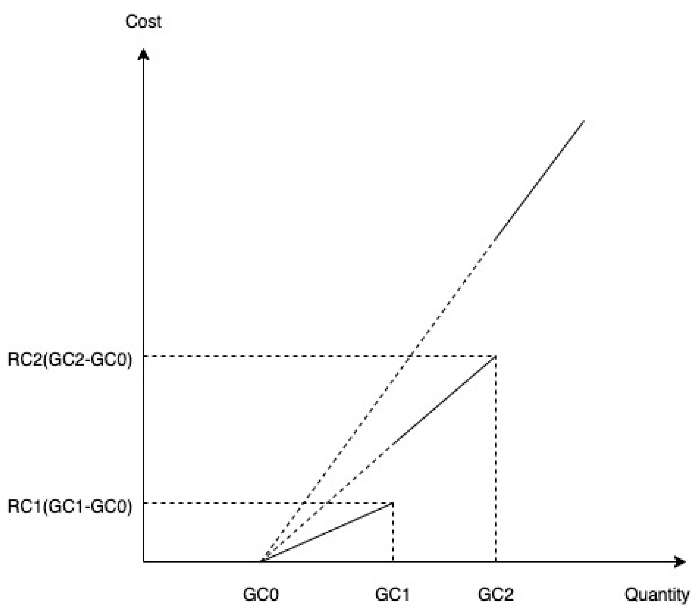
3.4.2. Continuous Progressive Tax Rate Carbon Tax Cost Function with Tax Exemption Quota (Including Carbon Rights Trading)

This model also takes into consideration the carbon emissions exempted from taxation by the government. Similar to Figure 4, as described in Functions (31)–(41), Functions (44)–(54) represent constraints associated with carbon tax costs, where carbon emissions from companies within the carbon emission limit are not subjected to taxation. However, once the exempted carbon emission threshold is surpassed, varying levels of carbon emissions correspond to different carbon tax rates. Additionally, this function incorporates the purchasing cost or selling revenue of carbon credits in carbon trading. Beyond this limit, varying carbon emissions incur different tax rates, and the function includes the cost of buying or income from selling carbon rights. Moreover, the total carbon cost of the function is $\left[\right(\left({GC}_1{\mathrm{\varnothing }}_1+{GC}_2{\mathrm{\varnothing }}_2+{GC}_3{\mathrm{\varnothing }}_3\right)-\left(UCE-g\right)\ast R){\omega }_1+(\left(G{C}_1{\mathrm{\varnothing }}_1+{GC}_2{\mathrm{\varnothing }}_2+{GC}_3{\mathrm{\varnothing }}_3\right)+\left(g-UCE\right)\ast R{)\omega }_2]$, as displayed in Function (43).

$$\begin{gathered} \mathsf{\pi }={\mathrm{P}}_1{\mathrm{X}}_{11}+{\mathrm{P}}_2{\mathrm{X}}_{21}+{\mathrm{P}}_3{\mathrm{X}}_{22}+{\mathsf{\beta }}_1\left(1-{\mathrm{e}}_1\right)\mathrm{M}+{\mathsf{\beta }}_2\left(1-{\mathrm{e}}_2\right){\mathrm{X}}_{12}+{\mathsf{\beta }}_3{\mathrm{e}}_3{\mathrm{X}}_{22} \\ -\left[\left({\mathrm{C}}_1\mathrm{M}+{\mathrm{C}}_2{\mathrm{m}}_{22\mathrm{d}}\right)+\left({\mathrm{C}}_3{\mathrm{m}}_{22\mathrm{c}}+{\mathrm{C}}_4{\mathrm{m}}_{22\mathrm{m}}\right)\right]-\left[{\mathcal{L}}_0+{\mathsf{\eta }}_1{\mathrm{r}}_{\mathrm{o}\mathrm{t}}\left({\mathrm{Q}}_1-{\mathrm{G}}_0\right)\right] \\ -\left[\right(\left({\mathrm{G}\mathrm{C}}_1{\mathrm{\varnothing }}_1+{\mathrm{G}\mathrm{C}}_2{\mathrm{\varnothing }}_2+{\mathrm{G}\mathrm{C}}_3{\mathrm{\varnothing }}_3\right)-\left(\mathrm{U}\mathrm{C}\mathrm{E}-\mathrm{g}\right)\ast \mathrm{R}){\mathsf{\omega }}_1 \\ +(\left(\mathrm{G}{\mathrm{C}}_1{\mathrm{\varnothing }}_1+{\mathrm{G}\mathrm{C}}_2{\mathrm{\varnothing }}_2+{\mathrm{G}\mathrm{C}}_3{\mathrm{\varnothing }}_3\right)+\left(\mathrm{g}-\mathrm{U}\mathrm{C}\mathrm{E}\right)\ast \mathrm{R}{)\mathsf{\omega }}_2] \\ +\left({\mathrm{C}}_5{\mathrm{R}\mathrm{E}}_{\mathrm{h}}+{\mathrm{C}}_6{\mathrm{R}\mathrm{E}}_{\mathrm{w}}\right)-\mathrm{F} \end{gathered}$$

(43)

$${\mathrm{q}}_{\mathrm{c}}{\mathrm{X}}_{22}\le {\mathrm{C}\mathrm{E}}_0+\left({\mathrm{C}\mathrm{E}}_1-{\mathrm{C}\mathrm{E}}_0\right){\mathrm{\varnothing }}_1+\left({\mathrm{C}\mathrm{E}}_2-{\mathrm{C}\mathrm{E}}_0\right){\mathrm{\varnothing }}_2+\left({\mathrm{C}\mathrm{E}}_3-{\mathrm{C}\mathrm{E}}_0\right){\mathrm{\varnothing }}_3$$

(44)

$${\mathrm{\varnothing }}_0-{\mathsf{\pi }}_1\le 0$$

(45)

$${\mathrm{\varnothing }}_1-{\mathsf{\pi }}_1-{\mathsf{\pi }}_2\le 0$$

(46)

$${\mathrm{\varnothing }}_2-{\mathsf{\pi }}_2-{\mathsf{\pi }}_3\le 0$$

(47)

$${\mathrm{\varnothing }}_3-{\mathsf{\pi }}_3\le 0$$

(48)

$${\mathrm{\varnothing }}_0+{\mathrm{\varnothing }}_1+{\mathrm{\varnothing }}_2+{\mathrm{\varnothing }}_3=1$$

(49)

$${\mathsf{\pi }}_1+{\mathsf{\pi }}_2+{\mathsf{\pi }}_3=1$$

(50)

$$0\le {\mathrm{\varnothing }}_0\le 1$$

(51)

$$0\le {\mathrm{\varnothing }}_1\le 1$$

(52)

$$0\le {\mathrm{\varnothing }}_2\le 1$$

(53)

$$0\le {\mathrm{\varnothing }}_3\le 1$$

(54)

$$\begin{gathered} {\mathrm{f}}_1\left(\mathrm{g}\right)=\left\{\begin{array}{cc}\hspace{1em}\hspace{1em}\hspace{1em}\hspace{1em} g \ast {\mathrm{R}\mathrm{C}}_1,& \mathrm{If} 0\le g\le {\mathrm{C}\mathrm{E}}_1\\ {\mathrm{G}\mathrm{C}}_1+\left(\mathrm{g}-{\mathrm{C}\mathrm{E}}_1\right){\mathrm{R}\mathrm{C}}_2,& \mathrm{If} {\mathrm{C}\mathrm{E}}_1<g\le {\mathrm{C}\mathrm{E}}_2\\ {\mathrm{G}\mathrm{C}}_2+\left(\mathrm{g}-{\mathrm{C}\mathrm{E}}_2\right){\mathrm{R}\mathrm{C}}_3,& \mathrm{If} {\mathrm{C}\mathrm{E}}_2<g\end{array}\right. \\ \mathrm{g}={\mathrm{q}}_{\mathrm{C}}{\mathrm{X}}_{22}={\mathrm{A}}_1+{\mathrm{A}}_2 \end{gathered}$$

(55)

$$0\le {\mathrm{A}}_1\le {\mathsf{\omega }}_1\mathrm{U}\mathrm{C}\mathrm{E}$$

(56)

$${\mathsf{\omega }}_2\mathrm{U}\mathrm{C}\mathrm{E}<{\mathrm{A}}_2\le {\mathsf{\omega }}_2\mathrm{U}\mathrm{C}\mathrm{C}\mathrm{E}$$

(57)

$${\mathsf{\omega }}_1+{\mathsf{\omega }}_2=1$$

(58)

In the above functions, we have the following:

${\mathrm{q}}_{\mathrm{c}}$	Total carbon emissions in the dyeing-and-finishing process;
${\mathrm{G}\mathrm{C}}_1$	First-stage total carbon tax cost;
${\mathrm{G}\mathrm{C}}_2$	Second-stage total carbon tax cost;
${\mathrm{G}\mathrm{C}}_3$	The total carbon tax cost of the third stage;
${\mathrm{C}\mathrm{E}}_0$	Carbon emissions from duty-free credits;
${\mathrm{C}\mathrm{E}}_1$	The total carbon emissions of the first stage;
${\mathrm{C}\mathrm{E}}_2$	The total carbon emissions of the second stage;
${\mathrm{C}\mathrm{E}}_3$	The total carbon emission of the third stage;
${\mathsf{\pi }}_1,{\mathsf{\pi }}_2,{\mathsf{\pi }}_3$	0, 1 dummy variable;
${\mathrm{\varnothing }}_0,{\mathrm{\varnothing }}_1,{\mathrm{\varnothing }}_2,{\mathrm{\varnothing }}_3$	A special set of non-negative variable types, at most two adjacent variables can be non-zero;
$\mathrm{U}\mathrm{C}\mathrm{E}$	Total National Carbon Emissions Cap.

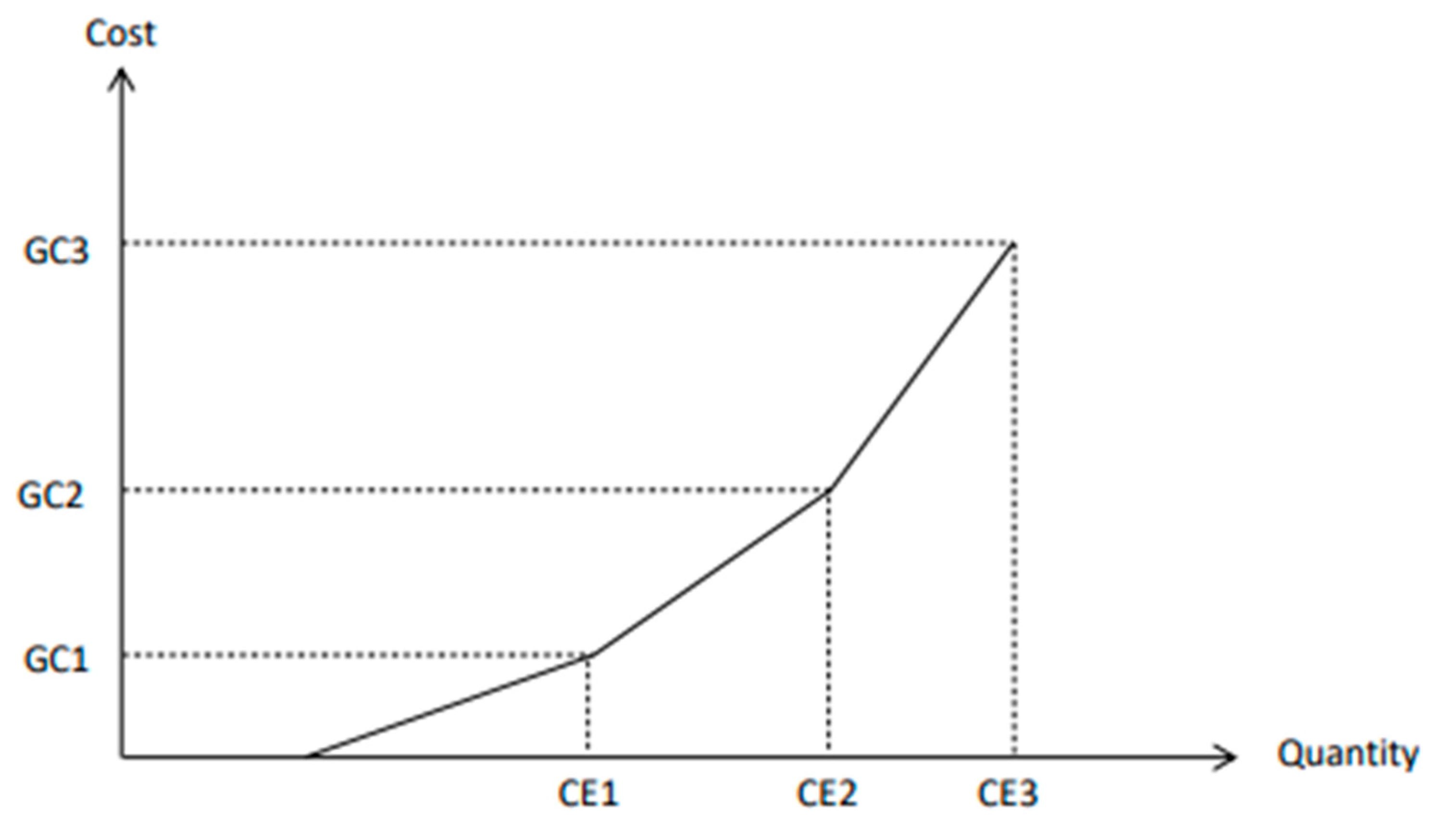
3.4.3. Tax Cost Function of Carbon with Discontinuous Progressive Tax Rate with Tax Exemption Quota

The carbon tax cost function for discontinuous progressive tax rates, accounting for government-granted untaxed carbon emissions is discussed in the provided sources. Enterprises’ carbon emissions are exempt from taxation within this limit. Beyond this limit, varying carbon emissions incur different tax rates. The function’s total carbon emission cost is $\left[{\delta }_1{RC}_1\left(C_1-{GC}_0\right)+{\delta }_2{RC}_2\left(C_2-{GC}_0\right)+{\delta }_3{RC}_3\left(C_3-{GC}_0\right)\right]$, as shown in Function (59). Functions (60)–(67) are constraints related to carbon tax costs:

$$\begin{gathered} \pi =P_1{X}_{11}+P_2{X}_{21}+P_3{X}_{22}+{\beta }_1\left(1-e_1\right)M+{\beta }_2\left(1-e_2\right)X_{12}+{\beta }_3{e}_3{X}_{22} \\ -\left[\left(C_{1}M+C_2{m}_{22d}\right)+\left(C_3{m}_{22c}+C_4{m}_{22m}\right)\right]-\left[{\mathcal{L}}_0+{\eta }_1{r}_{ot}\left(Q_1-G_0\right)\right] \\ -\left[{\delta }_1{RC}_1\left(C_1-{GC}_0\right)+{\delta }_2{RC}_2\left(C_2-{GC}_0\right)+{\delta }_3{RC}_3\left(C_3-{GC}_0\right)\right] \\ +\left(C_5{RE}_h+C_6{RE}_w\right)-F \end{gathered}$$

(59)

$$q_C{X}_{22}=C_0+C_1+C_2+C_3$$

(60)

$$0\le C_0\le {GC}_0{\delta }_0$$

(61)

$${\delta }_1{GC}_0<C_1\le {\delta }_1{GC}_1$$

(62)

$${\delta }_2{GC}_1<C_2\le {\delta }_2{GC}_2$$

(63)

$${\delta }_3{GC}_2<C_3$$

(64)

$${{\delta }_0+\delta }_1+{\delta }_2+{\delta }_3=1$$

(65)

$$q_c{X}_{22}\le UCE$$

(66)

In the above functions, we have the following:

${\mathrm{q}}_{\mathrm{c}}$	Total carbon emissions in the dyeing-and-finishing process;
${\mathrm{G}\mathrm{C}}_0$	Carbon emissions from duty-free credits;
${\mathrm{G}\mathrm{C}}_1$	First-stage total carbon tax cost;
${\mathrm{G}\mathrm{C}}_2$	Second-stage total carbon tax cost;
${\mathrm{G}\mathrm{C}}_3$	The total carbon tax cost of the third stage;
${\mathrm{C}}_0$	Not reaching the total carbon emissions for which a fee is charged;
${\mathrm{C}}_1$	The total carbon emissions of the first stage;
${\mathrm{C}}_2$	The total carbon emissions of the second stage;
${\mathrm{C}}_3$	The total carbon emission of the third stage;
${{\mathsf{\delta }}_0,\mathsf{\delta }}_1,{\mathsf{\delta }}_2,{\mathsf{\delta }}_3$	0, 1 dummy variable;
$\mathrm{U}\mathrm{C}\mathrm{E}$	National carbon cap.

3.4.4. Carbon Tax Cost Function with Discontinuous Progressive Tax Rate with Tax Exemption Quota (Including Carbon Rights Trading)

This model also represents the carbon tax cost function for discontinuous progressive tax rates. Similar to Figure 5, which is displayed in Functions (60)–(65), Functions (68)–(73) consider the government-granted untaxed carbon emissions. Within the limit, enterprises’ carbon emissions are exempt from taxation. Once the limit is exceeded, different levels of carbon emissions incur varying tax rates. This function also considers carbon rights trading, so the total carbon emission cost of this function is $\left\{\right[{\delta }_1{RC}_1\left(C_1-{GC}_0\right)+{\delta }_2{RC}_2\left(C_2-{GC}_0\right)+{\delta }_3{RC}_3\left(C_3-{GC}_0\right)-\left(UCE-g\right)\ast R]{\omega }_1+[{\delta }_1{RC}_1\left(C_1-{GC}_0\right)+{\delta }_2{RC}_2\left(C_2-{GC}_0\right)+{\delta }_3{RC}_3\left(C_3-{GC}_0\right)+\left(g-UCE\right)\ast R\left]{\omega }_2\right\}$, as displayed in Function (67).

$$\begin{gathered} \pi =P_1{X}_{11}+P_2{X}_{21}+P_3{X}_{22}+{\beta }_1\left(1-e_1\right)M+{\beta }_2\left(1-e_2\right)X_{12}+{\beta }_3{e}_3{X}_{22} \\ -\left[\left(C_{1}M+C_2{m}_{22d}\right)+\left(C_3{m}_{22c}+C_4{m}_{22m}\right)\right]-\left[{\mathcal{L}}_0+{\eta }_1{r}_{ot}\left(Q_1-G_0\right)\right] \\ -\left\{\right[{\delta }_1{RC}_1\left(C_1-{GC}_0\right)+{\delta }_2{RC}_2\left(C_2-{GC}_0\right)+{\delta }_3{RC}_3\left(C_3-{GC}_0\right)-\left(UCE-g\right) \ast R]{\omega }_1 \\ +[{\delta }_1{RC}_1\left(C_1-{GC}_0\right)+{\delta }_2{RC}_2\left(C_2-{GC}_0\right)+{\delta }_3{RC}_3\left(C_3-{GC}_0\right)+\left(g-UCE\right) \ast R]{\omega }_2\} \\ +\left(C_5{RE}_h+C_6{RE}_w\right)-F \end{gathered}$$

(67)

$$q_C{X}_{22}=C_0+C_1+C_2+C_3$$

(68)

$$0\le C_0\le {GC}_0{\delta }_1$$

(69)

$${GC}_0{\delta }_1<C_1\le {GC}_1{\delta }_1$$

(70)

$${GC}_1{\delta }_2<C_2\le {GC}_2{\delta }_2$$

(71)

$${GC}_2{\delta }_3<C_3$$

(72)

$${{\delta }_0+\delta }_1+{\delta }_2+{\delta }_3=1$$

(73)

$$g=q_C{X}_{22}=A_1+A_2$$

(74)

$$0\le A_1\le {\omega }_{1}UCE$$

(75)

$${\omega }_{2}UCE<A_2\le {\omega }_{2}UCCE$$

(76)

$${\omega }_{2}UCE<A_2\le {\omega }_{2}UCCE$$

(77)

In the above, we have the following:

${\mathrm{q}}_{\mathrm{c}}$	Total carbon emissions in the dyeing-and-finishing process;
${\mathrm{G}\mathrm{C}}_0$	Carbon emissions from duty-free credits;
${\mathrm{G}\mathrm{C}}_1$	First-stage total carbon tax cost;
${\mathrm{G}\mathrm{C}}_2$	Second-stage total carbon tax cost;
${\mathrm{G}\mathrm{C}}_3$	The total carbon tax cost of the third stage;
${\mathrm{C}}_0$	Not reaching the total carbon emissions for which a fee is charged
${\mathrm{C}}_1$	The total carbon emissions of the first stage;
${\mathrm{C}}_2$	The total carbon emissions of the second stage;
${\mathrm{C}}_3$	The total carbon emission of the third stage;
$\mathrm{U}\mathrm{C}\mathrm{E}$	National carbon cap;
$\mathrm{U}\mathrm{C}\mathrm{C}\mathrm{E}$	The maximum amount of carbon emissions that can be purchased;
$\mathrm{R}$	Single Carbon Right Cost Rate;
${\mathrm{A}}_1$	The company’s total carbon emissions when $\mathrm{g}\le \mathrm{U}\mathrm{C}\mathrm{E}$;
${\mathrm{A}}_2$	The company’s total carbon emissions when $\mathrm{g}>\mathrm{U}\mathrm{C}\mathrm{E}$;
${\mathsf{\omega }}_1,{\mathsf{\omega }}_2$	0, 1 dummy variable;
${\mathsf{\delta }}_0,{\mathsf{\delta }}_1,{\mathsf{\delta }}_2,{\mathsf{\delta }}_3$	0, 1 dummy variable.

4. Single-Period Model Analysis

4.1. Data Interpretation and Optimal Decision Analysis

Thesefour models assume a vertically integrated textile factory that produces three products using a single material, polyester fiber. The fiber is stretched and twisted to create textured yarn, some of which is sold. The remaining yarn is further processed to produce gray fabric, some of which is sold, and the rest is dyed and finished to yield high-priced fabric. The relevant costs in the model include (1) unit-level operations—material costs and labor costs; (2) batch-level operations—materials, product processing, and dyeing process settings; (3) environmental-level operations—carbon tax and energy recovery costs are divided into eight models in total; and (4) fixed costs—the depreciation, land, plant, and equipment are considered. The models aid companies in finding the optimal product mix to reduce production costs.

This article illustrates the utilization of the ABC (Activity-based Costing) method in a mathematical programming model for optimizing product-mix using the data presented in

Table 1. Sample data.

Activities Resource			Process 1		Process 2		Process 3
			Textured Yarn	Waste Yarn	Gray Cloth	Scrap Cloth	Finished Cloth	Eco-friendly Bricks
Selling Price Per Unit			TWD 97,000	TWD 570	TWD 135,000	TWD 2100	TWD 202,500	TWD 2300
Production Factor	$e_i$		0.96		0.95			0.14
	$(1-e_i)$		0.04		0.05
Direct Material Cost	$M,m_{22d}$		65,000				7000
	$m_{22c},m_{cem}$						1800	1500
Machine Hour Limit
Machine 1	Machine Hours	$h_i$	3
Machine 2					4
Machine 3							5
		$l_i$	3		2		1
Carbon Tax Limit	$q_c$	7
Direct Labor Constraints
Cost	$L_0=$ 47,840,000	$L_1$ = 101,660,000
Labor Hours	$G_0=\mathrm{368,000}$	$G_1=$ 598,000
Wage Rate	$W_{r0}=130/\mathrm{h}$	$W_{r1}=170/\mathrm{h}$
Carbon Tax Limit
Emissions	50,000	170,000	180,000
Tax Rate	800/ton	1100/ton	1500/ton

. Batch activities within the production process encompass the handling of materials and products from the process’s initiation to its conclusion. After each product is processed, it is returned to the factory for sale. This encompasses tasks such as adjusting dye settings during the dyeing and finishing phases. All the relevant data for this example are detailed in

Table 2. Sample data of batch handling.

Batch Job		Starting Point of Handling	Handling End Point	Textured Yarn	Gray Cloth	Finished Cloth
	${\mathsf{\sigma }}_{\mathbf{s}\mathbf{e}},{\mathbf{u}}_{\mathbf{s}\mathbf{e}}$	0	1	5,2
		1	2	1,1
		1	0	0.5,1
		2	3		1,1
		2	0		2,1
		3	0			3,2
	$\mathsf{\omega },\mathsf{\lambda }$					3,2

.

4.2. The Best Solution of One-Period Model 1

Table 3. Model data for Model 1 of green production model.

$\mathrm{M}\mathrm{a}\mathrm{x}\mathsf{\pi }=(\mathrm{97,000}\times {\mathrm{X}}_{11}+\mathrm{135,000}\times {\mathrm{X}}_{21}+\mathrm{202,500}\times {\mathrm{X}}_{22}+570\times 0.04\times \mathrm{M}$
$+2100\times 0.05\times {\mathrm{X}}_{12}+2300\times 0.14\times {\mathrm{X}}_{22})-(\mathrm{65,000}\times \mathrm{M}+7000\times {\mathrm{m}}_{22\mathrm{d}}$
$+1800\times {\mathrm{m}}_{22\mathrm{c}}+1500\times {\mathrm{m}}_{\mathrm{c}\mathrm{e}\mathrm{m}})-[\mathrm{47,840,000}+\left(170\times {\mathrm{Q}}_1-\mathrm{62,560,000}\times {\mathsf{\eta }}_1\right)]$
$-(\mathrm{40,000,000}\times \mathrm{\varnothing }1+\mathrm{172,000,000}\times \mathrm{\varnothing }2+\mathrm{187,000,000}\times \mathrm{\varnothing }3)$
$+\left(60\times \mathrm{R}\mathrm{E}\mathrm{h}+120\times \mathrm{R}\mathrm{E}\mathrm{w}\right)-\mathrm{50,000}$
Input–output relationship:	Machine hour objective function:
${\mathrm{X}}_1-0.96\times \mathrm{M}=0$	$3\times \mathrm{M}-\mathrm{120,000}\le 0$
${\mathrm{X}}_1={\mathrm{X}}_{11}+{\mathrm{X}}_{12}$	$4\times {\mathrm{X}}_{12}-\mathrm{100,000}\le 0$
${\mathrm{X}}_2-0.95\times {\mathrm{X}}_{12}=0$	$5\times {\mathrm{X}}_{22}-\mathrm{130,000}\le 0$
${\mathrm{B}\mathrm{P}}_2=0.05\times {\mathrm{X}}_{12}$	Batch-handling objective function:
${\mathrm{B}\mathrm{P}}_3=0.14\times {\mathrm{X}}_{22}$	$\mathrm{M}\le 5\times {\mathrm{B}}_{01}$
${\mathrm{m}}_{22\mathrm{d}}=0.65\times {\mathrm{X}}_{22}$	${\mathrm{X}}_{12}\le 1\times {\mathrm{B}}_{12}$
${\mathrm{m}}_{22\mathrm{c}}=0.1\times {\mathrm{X}}_{22}$	${\mathrm{X}}_{11}+0.04\times \mathrm{M}\le 0.5\times {\mathrm{B}}_{10}$
${\mathrm{m}}_{\mathrm{c}\mathrm{i}\mathrm{n}}=0.2\times {\mathrm{m}}_{22\mathrm{c}}$	${\mathrm{X}}_{22}\le 1\times {\mathrm{B}}_{23}$
${\mathrm{m}}_{\mathrm{c}\mathrm{e}\mathrm{m}}=6\times {\mathrm{m}}_{\mathrm{c}\mathrm{i}\mathrm{n}}$	${\mathrm{X}}_{21}+0.05\times {\mathrm{X}}_{12}\le 2\times {\mathrm{B}}_{20}$
${\mathrm{R}\mathrm{E}}_{\mathrm{h}}=0.95\times {\mathrm{X}}_{22}$	${\mathrm{X}}_{22}+0.14\times {\mathrm{X}}_{22}\le 3\times {\mathrm{B}}_{30}$
${\mathrm{R}\mathrm{E}}_{\mathrm{w}}=0.85\times {\mathrm{X}}_{22}$	${\mathrm{X}}_{22}\le 3\times \mathrm{B}\mathrm{S}$
Target carbon tax function:	Direct artificial objective function:
$7\times {\mathrm{X}}_{22}=\mathrm{10,000}+\left(\mathrm{60,000}-\mathrm{10,000}\right)$	$3\times \mathrm{M}+2\times {\mathrm{X}}_{12}+1\times {\mathrm{X}}_{22}+2\times {\mathrm{B}}_{01}$
$\times {\mathrm{D}}_1+\left(\mathrm{180,000}-\mathrm{10,000}\right){\times \mathrm{D}}_2$	$+1\times {\mathrm{B}}_{12}+1\times {\mathrm{B}}_{10}+1\times {\mathrm{B}}_{23}$
$+\left(\mathrm{190,000}-\mathrm{10,000}\right)\times {\mathrm{D}}_3$	$+1\times {\mathrm{B}}_{20}+2\times {\mathrm{Q}}_0\le {\mathsf{\eta }}_0\times \mathrm{368,000}$
$D_0-P_1\le 0$	${\mathrm{Q}}_0\le {\mathsf{\eta }}_0\times \mathrm{368,000}$
$D_1-P_1-P_2\le 0$	${\mathsf{\eta }}_1\times \mathrm{368,000}<{\mathrm{Q}}_1$
$D_2-P_2-P_3\le 0$	${\mathrm{Q}}_1\le {\mathsf{\eta }}_1\times \mathrm{598,000}$
$D_3-P_3\le 0$	${\mathsf{\eta }}_0+{\mathsf{\eta }}_1=1$
$D_0+D_1+D_2+D_3=1$
$P_1+P_2+P_3=1$
$0\le D_0\le 1$
$0\le D_1\le 1$
$0\le D_2\le 1$
$0\le D_3\le 1$
$P_1,P_2,P_3=\mathrm{0,1}$
$q_c{X}_{22}\le \mathrm{150,000}$

contains sample data for integer programming Model 1 (MIP) for a single period. The optimal solution, obtained using Lingo16.0, is presented in

Table 4. Model 1’s best solution.

$\pi =\mathrm{3,073,768,000}$	$X_1=\mathrm{38,400}$	$X_{11}=\mathrm{13,400}$	$X_{12}=\mathrm{25,000}$
$X_2=\mathrm{23,750}$	$X_{21}=2321.429$	$X_{22}=\mathrm{21,428.57}$	${BP}_1=1600$
${BP}_2=1250$	${BP}_3=3000$	$M=\mathrm{40,000}$	$m_{22d}=\mathrm{13,928.57}$
$m_{22c}=2142.857$	$m_{cin}=428.5714$	$m_{22m}=2571.429$	$Q_0=0$
$Q_1=\mathrm{368,000}$	${\eta }_0=0$	${\eta }_1=1$	${\mathrm{\varnothing }}_0=0$
${\mathrm{\varnothing }}_1=0.25$	${\mathrm{\varnothing }}_2=0.75$	${\mathrm{\varnothing }}_3=0$	$P_1=0$
$P_2=1$	$P_3=0$	${RE}_h=\mathrm{20,357.14}$	${RE}_w=\mathrm{18,214.29}$
$B_{01}=8000$	$B_{12}=\mathrm{25,000}$	$B_{10}=\mathrm{30,000}$	$B_{23}=\mathrm{21,428.57}$
$B_{20}=\mathrm{26,785.71}$	$B_{30}=8142.857$	$BS=7142.857$

, the optimal solution of the model indicates the optimal product mix. The profits of the three products and three by-products are TWD 3,073,768,000, and the product quantities are 13,400 (tons), 2321.429 (tons), and 21,428.57 (tons). The quantities of raw materials are 40,000 (tons), 13,925.57 (tons), and 2142.857 (tons). The heat recovery cost saved is TWD 1,221,428. The cost of recycling the saved water is TWD 2,185,715. The final carbon tax cost is TWD 139,000,000, and the carbon emissions are 150,000 (tons).

4.3. The Best Solution of the Second Single-Period Model

Table 5. Sample data for Model 2 of green production model.

$\mathrm{M}\mathrm{a}\mathrm{x}\mathsf{\pi }=(\mathrm{97,000}\times {\mathrm{X}}_{11}+\mathrm{135,000}\times {\mathrm{X}}_{21}+\mathrm{202,500}\times {\mathrm{X}}_{22}+570\times 0.04\times \mathrm{M}$
$+2100\times 0.05\times {\mathrm{X}}_{12}+2300\times 0.14\times {\mathrm{X}}_{22})-(\mathrm{65,000}\times \mathrm{M}+7000\times {\mathrm{m}}_{22\mathrm{d}}$
$+1800\times {\mathrm{m}}_{22\mathrm{c}}+1500\times {\mathrm{m}}_{\mathrm{c}\mathrm{e}\mathrm{m}})-[\mathrm{47,840,000}+\left(170\times {\mathrm{Q}}_1-\mathrm{62,560,000}\times {\mathsf{\eta }}_1\right)]$
$-[\mathrm{40,000,000}\times \mathrm{\varnothing }1+\mathrm{172,000,000}\times \mathrm{\varnothing }2+\mathrm{187,000,000}\times \mathrm{\varnothing }3-(\mathrm{150,000}-\left({\mathrm{A}}_1+{\mathrm{A}}_2\right))$
$\times 600]\times {\mathrm{K}}_1-[\mathrm{40,000,000}\times \mathrm{\varnothing }1+\mathrm{172,000,000}\times \mathrm{\varnothing }2+\mathrm{187,000,000}\times \mathrm{\varnothing }3$
$-\left(\left({\mathrm{A}}_1+{\mathrm{A}}_2\right)-\mathrm{150,000}\right)\times 600]\times {\mathrm{K}}_2+\left(60\times \mathrm{R}\mathrm{E}\mathrm{h}+120\times \mathrm{R}\mathrm{E}\mathrm{w}\right)-\mathrm{50,000}$
Input–output relationship:	Input–output relationship:
$X_1-0.96\times M=0$	$3\times M-\mathrm{120,000}\le 0$
$X_1=X_{11}+X_{12}$	$4\times X_{12}-\mathrm{100,000}\le 0$
$X_2-0.95\times X_{12}=0$	$5\times X_{22}-\mathrm{130,000}\le 0$
${\mathrm{B}\mathrm{P}}_2=0.05\times {\mathrm{X}}_{12}$	Batch-handling objective function:
${\mathrm{B}\mathrm{P}}_3=0.14\times {\mathrm{X}}_{22}$	$\mathrm{M}\le 5\times {\mathrm{B}}_{01}$
${\mathrm{m}}_{22\mathrm{d}}=0.65\times {\mathrm{X}}_{22}$	${\mathrm{X}}_{12}\le 1\times {\mathrm{B}}_{12}$
${\mathrm{m}}_{22\mathrm{c}}=0.1\times {\mathrm{X}}_{22}$	${\mathrm{X}}_{11}+0.04\times \mathrm{M}\le 0.5\times {\mathrm{B}}_{10}$
${\mathrm{m}}_{\mathrm{c}\mathrm{i}\mathrm{n}}=0.2\times {\mathrm{m}}_{22\mathrm{c}}$	${\mathrm{X}}_{22}\le 1\times {\mathrm{B}}_{23}$
${\mathrm{m}}_{\mathrm{c}\mathrm{e}\mathrm{m}}=6\times {\mathrm{m}}_{\mathrm{c}\mathrm{i}\mathrm{n}}$	${\mathrm{X}}_{21}+0.05\times {\mathrm{X}}_{12}\le 2\times {\mathrm{B}}_{20}$
${\mathrm{R}\mathrm{E}}_{\mathrm{h}}=0.95\times {\mathrm{X}}_{22}$	${\mathrm{X}}_{22}+0.14\times {\mathrm{X}}_{22}\le 3\times {\mathrm{B}}_{30}$
${\mathrm{R}\mathrm{E}}_{\mathrm{w}}=0.85\times {\mathrm{X}}_{22}$	${\mathrm{X}}_{22}\le 3\times \mathrm{B}\mathrm{S}$
Target carbon tax function:	Direct artificial objective function:
$7\times {\mathrm{X}}_{22}=\mathrm{10,000}+\left(\mathrm{60,000}-\mathrm{10,000}\right)$	$3\times \mathrm{M}+2\times {\mathrm{X}}_{12}+1\times {\mathrm{X}}_{22}+2\times {\mathrm{B}}_{01}$
$\times {\mathrm{D}}_1+\left(\mathrm{180,000}-\mathrm{10,000}\right)\times {\mathrm{D}}_2$	$+1\times {\mathrm{B}}_{12}+1\times {\mathrm{B}}_{10}+1\times {\mathrm{B}}_{23}$
$+\left(\mathrm{190,000}-\mathrm{10,000}\right)\times {\mathrm{D}}_3$	$+1\times {\mathrm{B}}_{20}+2\times {\mathrm{Q}}_0\le {\mathsf{\eta }}_0\times \mathrm{368,000}$
${\mathrm{D}}_0-{\mathrm{P}}_1\le 0$	${\mathrm{Q}}_0\le {\mathsf{\eta }}_0\times \mathrm{368,000}$
${\mathrm{D}}_1-{\mathrm{P}}_1-{\mathrm{P}}_2\le 0$	${\mathsf{\eta }}_1\times \mathrm{368,000}<{\mathrm{Q}}_1$
${\mathrm{D}}_2-{\mathrm{P}}_2-{\mathrm{P}}_3\le 0$	${\mathrm{Q}}_1\le {\mathsf{\eta }}_1\times \mathrm{598,000}$
${\mathrm{D}}_3-{\mathrm{P}}_3\le 0$	${\mathsf{\eta }}_0+{\mathsf{\eta }}_1=1$
${\mathrm{D}}_0+{\mathrm{D}}_1+{\mathrm{D}}_2+{\mathrm{D}}_3=1$
${\mathrm{P}}_1+{\mathrm{P}}_2+{\mathrm{P}}_3=1$
$0\le {\mathrm{D}}_0\le 1$
$0\le {\mathrm{D}}_1\le 1$
$0\le {\mathrm{D}}_2\le 1$
$0\le {\mathrm{D}}_3\le 1$
${\mathrm{P}}_1,{\mathrm{P}}_2,{\mathrm{P}}_3=\mathrm{0,1}$
${\mathrm{q}}_{\mathrm{c}}{\mathrm{X}}_{22}\le \mathrm{150,000}$
$7\times {\mathrm{X}}_{22}={\mathrm{A}}_1+{\mathrm{A}}_2$
${\mathrm{A}}_1\le {\mathrm{K}}_1\times \mathrm{150,000}$
${\mathrm{K}}_2\times \mathrm{150,000}<{\mathrm{A}}_2$
${\mathrm{A}}_2\le {\mathrm{K}}_2\times \mathrm{180,000}$
${\mathrm{K}}_1+{\mathrm{K}}_2=1$

contains sample data for integer programming Model 2 (MIP) for a single period.

The optimal solution, obtained using Lingo16.0, is presented in

Table 6. Model 2’s best solution.

$\pi =\mathrm{3,463,244,000}$	$X_1=\mathrm{38,400}$	$X_{11}=\mathrm{13,400}$	$X_{12}=\mathrm{25,000}$
$X_2=\mathrm{23,750}$	$X_{21}=1000$	$X_{22}=\mathrm{22,750}$	${BP}_1=1600$
${BP}_2=1250$	${BP}_3=3185$	$M=\mathrm{40,000}$	$m_{22d}=\mathrm{14,787.5}$
$m_{22c}=2275$	$m_{cin}=455$	$m_{22m}=2730$	$Q_0=0$
$Q_1=\mathrm{368,000}$	${\eta }_0=0$	${\eta }_1=1$	${\mathrm{\varnothing }}_0=0$
${\mathrm{\varnothing }}_1=0.1729$	${\mathrm{\varnothing }}_2=0.8271$	${\mathrm{\varnothing }}_3=0$	$P_1=0$
$P_2=1$	$P_3=0$	${RE}_h=\mathrm{21,612.5}$	${RE}_w=\mathrm{19,337.5}$
$B_{01}=8000$	$B_{12}=\mathrm{25,000}$	$B_{10}=\mathrm{30,000}$	$B_{23}=\mathrm{22,750}$
$B_{20}=\mathrm{24,521.67}$	$B_{30}=8645$	$BS=7583.333$

. The optimal solution in Table 6 represents the best product mix. The profits of the three products and three by-products are TWD 3,463,244,000, and the product quantities are 13,400 (tons), 1000 (tons), and 22,750 (tons). The quantities of raw materials are 40,000 (tons), 14,787.5 (tons), and 2275 (tons). The heat recovery cost saved is TWD 1,296,750. The cost of recycling the saved water is TWD 2,320,500. The final carbon tax cost is TWD 154,714,000, and the carbon emissions are 159,250 (tons).

4.4. The Best Solution of the Third Single-Period Model

Table 7. Sample data for Model 3 of green production model.

$\mathrm{M}\mathrm{a}\mathrm{x}\mathsf{\pi }=(\mathrm{97,000}\times {\mathrm{X}}_{11}+\mathrm{135,000}\times {\mathrm{X}}_{21}+\mathrm{202,500}\times {\mathrm{X}}_{22}+570\times 0.04\times \mathrm{M}$
$+2100\times 0.05\times {\mathrm{X}}_{12}+2300\times 0.14\times {\mathrm{X}}_{22})-(\mathrm{65,000}\times \mathrm{M}+7000\times {\mathrm{m}}_{22\mathrm{d}}$
$+1800\times {\mathrm{m}}_{22\mathrm{c}}+1500\times {\mathrm{m}}_{\mathrm{c}\mathrm{e}\mathrm{m}})-[\mathrm{47,840,000}+\left(170\times {\mathrm{Q}}_1-\mathrm{62,560,000}\times {\mathsf{\eta }}_1\right)]$
$-[{\mathrm{D}}_1\times 800\times \left({\mathrm{C}}_1-\mathrm{10,000}\right)+{\mathrm{D}}_2\times 1100\times \left({\mathrm{C}}_2-\mathrm{10,000}\right)+{\mathrm{D}}_3\times 1500\times$
$\left({\mathrm{C}}_3-\mathrm{10,000}\right)$]$+\left(60\times \mathrm{R}\mathrm{E}\mathrm{h}+120\times \mathrm{R}\mathrm{E}\mathrm{w}\right)-\mathrm{50,000}$
Input–output relationship:	Machine hour objective function:
${\mathrm{X}}_1-0.96\times \mathrm{M}=0$	$3\times \mathrm{M}-\mathrm{120,000}\le 0$
${\mathrm{X}}_1={\mathrm{X}}_{11}+{\mathrm{X}}_{12}$	$4\times {\mathrm{X}}_{12}-\mathrm{100,000}\le 0$
${\mathrm{X}}_2-0.95\times {\mathrm{X}}_{12}=0$	$5\times {\mathrm{X}}_{22}-\mathrm{130,000}\le 0$
${\mathrm{B}\mathrm{P}}_2=0.05\times {\mathrm{X}}_{12}$	Batch-handling objective function:
${\mathrm{B}\mathrm{P}}_3=0.14\times {\mathrm{X}}_{22}$	$\mathrm{M}\le 5\times {\mathrm{B}}_{01}$
${\mathrm{m}}_{22\mathrm{d}}=0.65\times {\mathrm{X}}_{22}$	${\mathrm{X}}_{12}\le 1\times {\mathrm{B}}_{12}$
${\mathrm{m}}_{22\mathrm{c}}=0.1\times {\mathrm{X}}_{22}$	${\mathrm{X}}_{11}+0.04\times \mathrm{M}\le 0.5\times {\mathrm{B}}_{10}$
${\mathrm{m}}_{\mathrm{c}\mathrm{i}\mathrm{n}}=0.2\times {\mathrm{m}}_{22\mathrm{c}}$	${\mathrm{X}}_{22}\le 1\times {\mathrm{B}}_{23}$
${\mathrm{m}}_{\mathrm{c}\mathrm{e}\mathrm{m}}=6\times {\mathrm{m}}_{\mathrm{c}\mathrm{i}\mathrm{n}}$	${\mathrm{X}}_{21}+0.05\times {\mathrm{X}}_{12}\le 2\times {\mathrm{B}}_{20}$
${\mathrm{R}\mathrm{E}}_{\mathrm{h}}=0.95\times {\mathrm{X}}_{22}$	${\mathrm{X}}_{22}+0.14\times {\mathrm{X}}_{22}\le 3\times {\mathrm{B}}_{30}$
${\mathrm{R}\mathrm{E}}_{\mathrm{w}}=0.85\times {\mathrm{X}}_{22}$	${\mathrm{X}}_{22}\le 3\times \mathrm{B}\mathrm{S}$
Target carbon tax function:	Direct artificial objective function:
$7\times X_{22}=C_0+C_1+C_2+C_3$	$3\times \mathrm{M}+2\times {\mathrm{X}}_{12}+1\times {\mathrm{X}}_{22}+2\times {\mathrm{B}}_{01}$
$C_0\le {\mathsf{\delta }}_0\times \mathrm{50,000}$	$+1\times {\mathrm{B}}_{12}+1\times {\mathrm{B}}_{10}+1\times {\mathrm{B}}_{23}$
$\mathrm{50,000}\times {\mathsf{\delta }}_1<C_1$	$+1\times {\mathrm{B}}_{20}+2\times {\mathrm{Q}}_0\le {\mathsf{\eta }}_0\times \mathrm{368,000}$
$C_1\le {\mathsf{\delta }}_1\times \mathrm{170,000}$	${\mathrm{Q}}_0\le {\mathsf{\eta }}_0\times \mathrm{368,000}$
${\mathsf{\delta }}_2\times \mathrm{170,000}\le C_2$	${\mathsf{\eta }}_1\times \mathrm{368,000}<{\mathrm{Q}}_1$
$C_2<{\mathsf{\delta }}_2\times \mathrm{180,000}$
${\mathsf{\delta }}_3\times \mathrm{180,000}<C_3$
$C_3\le {\mathsf{\delta }}_3\times 0.1E+10$
${\mathsf{\delta }}_1+{\mathsf{\delta }}_2+{\mathsf{\delta }}_3+{\mathsf{\delta }}_4=1$
$q_c{X}_{22}\le \mathrm{150,000}$

contains sample data for integer programming Model 3 (MIP) for a single period.

The optimal solution, obtained using Lingo16.0, is presented in

Table 8. The best solution of Model 3.

$\pi =\mathrm{3,100,768,000}$	$X_1=\mathrm{38,400}$	$X_{11}=\mathrm{13,400}$	$X_{12}=\mathrm{25,000}$
$X_2=\mathrm{23,750}$	$X_{21}=2321.429$	$X_{22}=\mathrm{21,428.57}$	${BP}_1=1600$
${BP}_2=1250$	${BP}_3=3000$	$M=\mathrm{40,000}$	$m_{22d}=\mathrm{13,928.57}$
$m_{22c}=2142.857$	$m_{cin}=428.5714$	$m_{cem}=2571.43$	$Q_0=0$
$Q_1=\mathrm{368,000}$	${\eta }_0=0$	${\eta }_1=1$	$C_0=0$
$C_1=\mathrm{150,000}$	$C_2=0$	$C_3=0$	${\delta }_0=0$
${\delta }_1=0$	${\delta }_2=1$	${\delta }_3=0$	${RE}_h=\mathrm{20,357.14}$
${RE}_w=\mathrm{18,214.29}$	$B_{01}=8000$	$B_{12}=\mathrm{25,000}$	$B_{10}=\mathrm{30,000}$
$B_{23}=\mathrm{21,428.57}$	$B_{20}=\mathrm{26,785.71}$	$B_{30}=8142.857$	$BS=7142.857$

. The optimal solution in Table 8 represents the best product mix. The profits of the three products and three by-products are TWD 3,100,768,000, and the product quantities are 13,400 (tons), 2321.429 (tons), and 21,428.57 (tons). The quantities of raw materials are 40,000 (tons), 13,928.57 (tons), and 2142.857 (tons). The heat recovery cost saved is TWD 1,221,428. The cost of recycling the saved water is TWD 2,185,715. The final carbon tax cost is TWD 112,000,000 and the carbon emissions are 150,000 (tons).

4.5. The Best Solution of the Fourth Single-Period Model

Table 9. Sample data for Model 4 of green production model.

$\mathrm{M}\mathrm{a}\mathrm{x}\mathsf{\pi }=(\mathrm{97,000}\times {\mathrm{X}}_{11}+\mathrm{135,000}\times {\mathrm{X}}_{21}+\mathrm{202,500}\times {\mathrm{X}}_{22}+570\times 0.04\times \mathrm{M}$
$+2100\times 0.05\times {\mathrm{X}}_{12}+2300\times 0.14\times {\mathrm{X}}_{22})-(\mathrm{65,000}\times \mathrm{M}+7000\times {\mathrm{m}}_{22\mathrm{d}}$
$+1800\times {\mathrm{m}}_{22\mathrm{c}}+1500\times {\mathrm{m}}_{\mathrm{c}\mathrm{e}\mathrm{m}})-[\mathrm{47,840,000}+\left(170\times {\mathrm{Q}}_1-\mathrm{62,560,000}\times {\mathsf{\eta }}_1\right)]$
$-[{\mathrm{D}}_1\times 800\times \left({\mathrm{C}}_1-\mathrm{10,000}\right)+{\mathrm{D}}_2\times 1100\times \left({\mathrm{C}}_2-\mathrm{10,000}\right){\mathrm{D}}_3\times 1500\times \left({\mathrm{C}}_3-\mathrm{10,000}\right)$
$-\left(\mathrm{150,000}-\left({\mathrm{A}}_1+{\mathrm{A}}_2\right)\right)\times 600]\times {\omega }_1-[{\mathrm{D}}_1\times 800\times \left({\mathrm{C}}_1-\mathrm{10,000}\right)+{\mathrm{D}}_2\times 1100$
$\times \left({\mathrm{C}}_2-\mathrm{10,000}\right)+{\mathrm{D}}_3\times 1500\times \left({\mathrm{C}}_3-\mathrm{10,000}\right)+\left(\left({\mathrm{A}}_1+{\mathrm{A}}_2\right)-\mathrm{150,000}\right)\times 600]\times {\omega }_2$
$+\left(60\times \mathrm{R}\mathrm{E}\mathrm{h}+120\times \mathrm{R}\mathrm{E}\mathrm{w}\right)-\mathrm{50,000}$
Input–output relationship:	Machine hour objective function:
${\mathrm{X}}_1-0.96\times \mathrm{M}=0$	$3\times \mathrm{M}-\mathrm{120,000}\le 0$
${\mathrm{X}}_1={\mathrm{X}}_{11}+{\mathrm{X}}_{12}$	$4\times {\mathrm{X}}_{12}-\mathrm{100,000}\le 0$
${\mathrm{X}}_2-0.95\times {\mathrm{X}}_{12}=0$	$5\times {\mathrm{X}}_{22}-\mathrm{130,000}\le 0$
${\mathrm{B}\mathrm{P}}_2=0.05\times {\mathrm{X}}_{12}$	Batch-handling objective function:
${\mathrm{B}\mathrm{P}}_3=0.14\times {\mathrm{X}}_{22}$	$\mathrm{M}\le 5\times {\mathrm{B}}_{01}$
${\mathrm{m}}_{22\mathrm{d}}=0.65\times {\mathrm{X}}_{22}$	${\mathrm{X}}_{12}\le 1\times {\mathrm{B}}_{12}$
${\mathrm{m}}_{22\mathrm{c}}=0.1\times {\mathrm{X}}_{22}$	${\mathrm{X}}_{11}+0.04\times \mathrm{M}\le 0.5\times {\mathrm{B}}_{10}$
${\mathrm{m}}_{\mathrm{c}\mathrm{i}\mathrm{n}}=0.2\times {\mathrm{m}}_{22\mathrm{c}}$	${\mathrm{X}}_{22}\le 1\times {\mathrm{B}}_{23}$
${\mathrm{m}}_{\mathrm{c}\mathrm{e}\mathrm{m}}=6\times {\mathrm{m}}_{\mathrm{c}\mathrm{i}\mathrm{n}}$	${\mathrm{X}}_{21}+0.05\times {\mathrm{X}}_{12}\le 2\times {\mathrm{B}}_{20}$
${\mathrm{R}\mathrm{E}}_{\mathrm{h}}=0.95\times {\mathrm{X}}_{22}$	${\mathrm{X}}_{22}+0.14\times {\mathrm{X}}_{22}\le 3\times {\mathrm{B}}_{30}$
${\mathrm{R}\mathrm{E}}_{\mathrm{w}}=0.85\times {\mathrm{X}}_{22}$	${\mathrm{X}}_{22}\le 3\times \mathrm{B}\mathrm{S}$
Target carbon tax function:	Direct artificial objective function:
$7\times {\mathrm{X}}_{22}={\mathrm{C}}_0+{\mathrm{C}}_1+{\mathrm{C}}_2+{\mathrm{C}}_3$	$3\times \mathrm{M}+2\times {\mathrm{X}}_{12}+1\times {\mathrm{X}}_{22}+2\times {\mathrm{B}}_{01}$
${\mathrm{C}}_0\le {\mathsf{\delta }}_0\times \mathrm{50,000}$	$+1\times {\mathrm{B}}_{12}+1\times {\mathrm{B}}_{10}+1\times {\mathrm{B}}_{23}$
$\mathrm{50,000}\times {\mathsf{\delta }}_1<{\mathrm{C}}_1$	$+1\times {\mathrm{B}}_{20}+2\times {\mathrm{Q}}_0\le {\mathsf{\eta }}_0\times \mathrm{36,8000}$
${\mathrm{C}}_1\le {\mathsf{\delta }}_1\times \mathrm{170,000}$	${\mathrm{Q}}_0\le {\mathsf{\eta }}_0\times \mathrm{36,8000}$
${\mathsf{\delta }}_2\times \mathrm{170,000}\le {\mathrm{C}}_2$	${\mathsf{\eta }}_1\times \mathrm{36,8000}<{\mathrm{Q}}_1$
${\mathrm{C}}_2<{\mathsf{\delta }}_2\times \mathrm{180,000}$
${\mathsf{\delta }}_3\times \mathrm{180,000}<{\mathrm{C}}_3$
${\mathrm{C}}_3\le {\mathsf{\delta }}_3\times 0.1\mathrm{E}+10$
${\mathsf{\delta }}_0+{\mathsf{\delta }}_1+{\mathsf{\delta }}_2+{\mathsf{\delta }}_3=1$
${\mathrm{q}}_{\mathrm{c}}{\mathrm{X}}_{22}\le \mathrm{150,000}$
$7\times {\mathrm{X}}_{22}={\mathrm{A}}_1+{\mathrm{A}}_2$
${\mathrm{A}}_1\le {\mathrm{K}}_1\times \mathrm{150,000}$
${\mathrm{K}}_2\times \mathrm{150,000}<{\mathrm{A}}_2$
${\mathrm{A}}_2\le {\mathrm{K}}_2\times \mathrm{180,000}$
${\mathrm{K}}_1+{\mathrm{K}}_2=1$

contains sample data for integer programming Model 4 (MIP) for a single period.

The optimal solution, obtained using Lingo16.0, is presented in

Table 10. Model 4’s best solution.

$\pi =\mathrm{3,171,162,000}$	$X_1=\mathrm{38,400}$	$X_{11}=\mathrm{13,400}$	$X_{12}=\mathrm{25,000}$
$X_2=\mathrm{23,750}$	$X_{21}=1000$	$X_{22}=\mathrm{22,750}$	${BP}_1=1600$
${BP}_2=1250$	${BP}_3=3185$	$M=\mathrm{40,000}$	$m_{22d}=\mathrm{14,787.5}$
$m_{22c}=2275$	$m_{cin}=455$	$m_{cem}=2730$	$Q_0=0$
$Q_1=\mathrm{368,000}$	${\eta }_0=0$	${\eta }_1=1$	$C_0=0$
$C_1=\mathrm{159,250}$	$C_2=0$	$C_3=0$	${\delta }_0=0$
${\delta }_1=1$	${\delta }_2=0$	${\delta }_3=0$	${RE}_h=\mathrm{21,612.5}$
${RE}_w=\mathrm{19,337.5}$	$B_{01}=8000$	$B_{12}=\mathrm{25,000}$	$B_{10}=\mathrm{76,793.33}$
$B_{23}=\mathrm{22,750}$	$B_{20}=1125$	$B_{30}=8645$	$BS=7583.33$
$A_1=0$	$A_2=\mathrm{159,250}$	${\omega }_1=0$	${\omega }_2=1$

. The optimal solution in Table 10 represents the best product mix. The profits of the three products and three by-products are TWD 3,171,162,000, and the product quantities are 13,400 (tons), 1000 (tons), and 22,750 (tons). The quantities of raw materials are 40,000 (tons), 14,787.5 (tons), and 2275 (tons). The heat recovery cost saved is TWD 1,296,750. The cost of recycling the saved water is TWD 2,320,500. The final carbon tax cost is TWD 124,950,000, and the carbon emissions are 159,250 (tons).

4.6. Single-Period Model Comparison

Table 11. Comparison table of various models in a single period.

Model	Profit	Carbon Emission	Carbon Tax cost	Main Product Quantity (X11)	Main Product Quantity (X21)	Main Product Quantity (X22)	Heat Recovery Benefits	Water Recycling Benefits
Model 1	3,073,768,000	150,000	139,000,000	13,400	2321.429	21,428.57	1,221,428	2,185,715
Model 2	3,463,244,000	159,250	154,714,000	13,400	1000	22,750	1,296,750	2,320,500
Model 3	3,100,768,000	150,000	112,000,000	13400	2321.429	21,428.57	1,221,428	2,185,715
Model 4	3,171,162,000	159,250	124,950,000	13,400	1000	22,750	1,296,750	2,320,500

Note: Models 1, 2, 3, and 4 use the data in Table 4, Table 5, Table 6, Table 7, Table 8, Table 9 and Table 10.

compares key parameters for each model in a single period, including profit, carbon emission, carbon tax cost, quantity of main products, and recovery income for heat and water energy. Models 2 and 4, which include carbon rights trading, are highlighted in the table. We can see that the two models both purchase carbon rights, and Model 2 (TWD 3,463,244,000) has the highest profit in the continuous progressive tax rate model. Among the discontinuous progressive tax rate models, Model 4 (TWD 3,171,162,000) is the most profitable.

5. Multi-Period Models

5.1. Model Functions

In Section 3, we introduced a one-period model. However, in reality, enterprises operate over multiple periods. Therefore, we extend the model in this section to include time considerations. We add a subscript t to represent different periods and consider the availability of stored raw materials and carbon rights for use in future periods. We also introduce additional constraints and functions, such as the unit direct labor cost, batch cost transfer, and input–output relationships. Models 2 to 4 focus on the carbon tax cost function only.

5.2. Carbon Tax Cost Function of Continuous Incremental Tax Rate with Tax Exemption Quota

5.2.1. Objective Equation

This model extends the objective equation of single-period Model 1 to multiple periods, using a subscript t to represent each period and considering tax-free allowances.

$$\pi =\sum _{t=1}^T\left[P_1{X}_{11t}+P_2{X}_{21t}+P_3{X}_{22t}+{\beta }_1\left(1-e_1\right)M_t+{\beta }_2\left(1-e_2\right)X_{12t}+{\beta }_3{e}_3{X}_{22t}\right]$$

$$-\sum _{t=1}^T\left[\left(C_1{M}_t+C_2{m}_{22dt}\right)+\left(C_3{m}_{22ct}+C_4{m}_{22mt}\right)\right]-\sum _{t=1}^T\left[L_0+{\eta }_{1t}{r}_{ot}\left(Q_{1t}-G_0\right)\right]$$

(78)

$$-\sum _{t=1}^T\left({GC}_1{\mathrm{\varnothing }}_{1t}+{GC}_2{\mathrm{\varnothing }}_{2t}+{GC}_3{\mathrm{\varnothing }}_{3t}\right)+\sum _{t=1}^T\left(C_5{RE}_{ht}+C_6{RE}_{wt}\right)-\sum _{t=1}^T{F}_t$$

5.2.2. Unit Direct Labor Cost Constraint

This constraint extends the single-period direct labor cost constraint from Section 3 to a multi-period labor cost constraint.

$$\sum _{t=1}^T(l_1{X}_{1t}+l_2{X}_{2t}+l_3{X}_{22t}+{\mu }_{01}{B}_{01t}+{\mu }_{12}{B}_{12t}+{\mu }_{10}{B}_{10t}+{\mu }_{23}{B}_{23t}$$

$$+{\mu }_{20}{B}_{20t}+{\mu }_{30}{B}_{30t}+\omega {BS}_t)=\sum _{t=1}^T\left(Q_{0t}+Q_{1t}\right)$$

(79)

$$0\le Q_{0t}\le {\eta }_{0t}{G}_0,t=1,2,3$$

(80)

$${\eta }_{1t}{G}_0<Q_{1t}\le {\eta }_{1t}{G}_1,t=1,2,3$$

(81)

$${\eta }_{0t}+{\eta }_{1t}=1,t=1,2,3$$

(82)

5.2.3. Batch Cost Handling Constraints

Extend the single-phase batch-handling constraint from Section 3 to a multiphase batch-handling constraint.

$${\mathrm{M}}_{\mathrm{t}}\le {\mathsf{\sigma }}_{01}{\mathrm{B}}_{01\mathrm{t}},\mathrm{t}=1,2,3$$

(83)

$${\mathrm{X}}_{12\mathrm{t}}\le {\mathsf{\sigma }}_{12}{\mathrm{B}}_{12\mathrm{t}},\mathrm{t}=1,2,3$$

(84)

$$X_{11t}+\left(1-e_1\right)M_t\le {\sigma }_{10}{B}_{10t} ,t=1,2,3$$

(85)

$$X_{22t}\le {\sigma }_{23}{B}_{23t} ,t=1,2,3$$

(86)

$$X_{21t}+\left(1-e_2\right)X_{12t}\le {\sigma }_{20}{B}_{20t} ,t=1,2,3$$

(87)

$$X_{22t}+e_3{X}_{22t}\le {\sigma }_{30}{B}_{30t} ,t=1,2,3$$

(88)

$$X_{22t}\le \lambda {BS}_t ,t=1,2,3$$

(89)

5.2.4. Restricted Heat and Water Energy Recovery

The multistage heat and water energy recovery restriction is an extension of the single-stage heat and water recovery constraint discussed in Section 3.

$${RE}_{ht}={\rho }_1\times X_{22t},t=1,2,3$$

(90)

$${RE}_{wt}={\rho }_2\times X_{22t},t=1,2,3$$

(91)

5.2.5. Restricted Formula of Input–Output Relationship

Extend the input–output relationship constraint from the single period to the multi-period as an extension of the constraint mentioned in Section 3.

$$X_{1t}-e_1{M}_t=0,t=1,2,3$$

(92)

$$X_{1t}=X_{11t}+X_{12t},t=1,2,3$$

(93)

$$X_{2t}-e_2{X}_{12t}=0,t=1,2,3$$

(94)

$$X_{2t}=X_{21t}+X_{22t},t=1,2,3$$

(95)

$$X_{12t}=e_2{X}_{12t}+\left(1-e_2\right)X_{12t},t=1,2,3$$

(96)

$${BP}_{1t}=\left(1-e_1\right)M_t,t=1,2,3$$

(97)

$${BP}_{2t}=\left(1-e_2\right)X_{12t},t=1,2,3$$

(98)

$${BP}_{3t}=e_3{X}_{22t},t=1,2,3$$

(99)

$$m_{22dt}={\vartheta }_1\times X_{22t},t=1,2,3$$

(100)

$$m_{22ct}={\vartheta }_2\times X_{22t},t=1,2,3$$

(101)

$$m_{cint}={\vartheta }_3\times m_{22ct},t=1,2,3$$

(102)

$$m_{22mt}={\vartheta }_4\times m_{cint},t=1,2,3$$

(103)

5.2.6. Other Sales and Production Restrictions

This is an extension of the other sales and production constraints mentioned in Section 3, applied to multi-period scenarios:

$$h_1{X}_{1t}\le H_1,t=1,2,3$$

(104)

$$h_2{X}_{2t}\le H_2,t=1,2,3$$

(105)

$$h_3{X}_{22t}\le H_{22},t=1,2,3$$

(106)

5.2.7. Carbon Tax Cost Constraints

Extension of carbon tax cost constraint from Model 1 in Section 3. The main difference is in the MQ part, where the total MQ is assumed, and carbon emissions can be freely deployed in three periods. The part of total carbon emissions is $q_c{X}_{22t}\le {CE}_0+\left({CE}_1-{CE}_0\right){\varnothing }_{1t}+\left({CE}_2-{CE}_0\right){\varnothing }_{2t}+\left({CE}_3-{CE}_0\right){\varnothing }_{3t}$.

$$q_c{X}_{22t}\le {CE}_0+\left({CE}_1-{CE}_0\right){\mathrm{\varnothing }}_{1t}+\left({CE}_2-{CE}_0\right){\mathrm{\varnothing }}_{2t}+\left({CE}_3-{CE}_0\right){\mathrm{\varnothing }}_{3t}$$

(107)

$$t=1,2,3$$

$$\sum _{t=1}^T{q}_c{X}_{22t}\le MQ$$

(108)

$${\mathrm{\varnothing }}_{0t}-{\pi }_{1t}\le 0,t=1,2,3$$

(109)

$${\mathrm{\varnothing }}_{1t}-{\pi }_{1t}-{\pi }_{2t}\le 0,t=1,2,3$$

(110)

$${\mathrm{\varnothing }}_{2t}-{\pi }_{2t}-{\pi }_{3t}\le 0,t=1,2,3$$

(111)

$${\mathrm{\varnothing }}_{3t}-{\pi }_{3t}\le 0,t=1,2,3$$

(112)

$${\pi }_{1t}+{\pi }_{2t}+{\pi }_{3t}=1 t=1,2,3$$

(113)

$${\pi }_{1t},{\pi }_{2t},{\pi }_{3t}=\mathrm{0,1},t=1,2,3$$

(114)

$${\mathrm{\varnothing }}_{0t}+{\mathrm{\varnothing }}_{1t}+{\mathrm{\varnothing }}_{2t}+{\mathrm{\varnothing }}_{3t}=1,t=1,2,3$$

(115)

$$0\le {\mathrm{\varnothing }}_{0t},{\mathrm{\varnothing }}_{1t},{\mathrm{\varnothing }}_{2t},{\mathrm{\varnothing }}_{3t}\le 1,t=1,2,3$$

(116)

Variable definition:

$MQ$—The maximum amount of carbon emissions without purchasing carbon rights in the third period.

5.2.8. Raw Material Restriction Formula

This restriction is a restriction on raw materials. We assumed the total amount of MM and allowed the raw materials to be allocated freely during the three periods.

$$\sum _{\mathrm{t}=1}^{\mathrm{T}}{\mathrm{M}}_{\mathrm{t}}=\mathrm{M}\mathrm{M} ,t=1,2,3$$

(117)

$$\mathrm{M}\mathrm{M}\le \mathrm{D}\mathrm{M}$$

(118)

Variable definition:

• $MM$—The sum of the raw materials required for the three phases;
• $DM$—The maximum volume of raw materials used in the three phases.

5.3. Carbon Tax Cost Function of Continuous Incremental Tax Rate with Tax Exemption Quota (Including Carbon Trading)

5.3.1. Objective Equation

This model extends the objective equation of the single-period Model 2 to a multi-period, using a subscript t for unknown variables to represent multiple periods, while considering tax-free allowances. Carbon emissions in all three periods are examined together to determine the need for carbon rights purchase. MQ represents the maximum amount of carbon emissions that can be made without purchasing carbon rights in the third period.

$$\pi =\sum _{t=1}^T\begin{array}{c}\left[P_1{X}_{11t}+P_2{X}_{21t}+P_3{X}_{22t}+{\beta }_1\left(1-e_1\right)M_t+{\beta }_2\left(1-e_2\right)X_{12t}+{\beta }_3{e}_3{X}_{22t}\right]\\ \\ \end{array}$$

$$-\sum _{t=1}^T\left[\left(C_1{M}_t+C_2{m}_{22dt}\right)+\left(C_3{m}_{22ct}+C_4{m}_{22mt}\right)\right]-\sum _{t=1}^T\left[L_0+{\eta }_{1t}{r}_{ot}\left(Q_{1t}-G_0\right)\right]$$

$$\sum _{t=1}^T[\left({GC}_1{\mathrm{\varnothing }}_{1t}+{GC}_2{\mathrm{\varnothing }}_{2t}+{GC}_3{\mathrm{\varnothing }}_{3t}\right)-R\ast (MQ-\sum _{t=1}^T{q}_c{X}_{22t}\left)\right]\ast {\omega }_1$$

(119)

$$\sum _{t=1}^T[\left({GC}_1{\mathrm{\varnothing }}_{1t}+{GC}_2{\mathrm{\varnothing }}_{2t}+{GC}_3{\mathrm{\varnothing }}_{3t}\right)+R\ast (\sum _{t=1}^T{q}_c{X}_{22t}-MQ\left)\right]\ast {\omega }_2$$

$$+\sum _{t=1}^T\left(C_5{RE}_{ht}+C_6{RE}_{wt}\right)-\sum _{t=1}^T{F}_t$$

5.3.2. Carbon Tax Cost Constraints

This constraint is an extension of the carbon tax cost constraint we mentioned in Model 4 of Section 3, where the part of the total carbon emissions is $q_c{X}_{22t}\le {CE}_0+\left({CE}_1-{CE}_0\right){\varnothing }_{1t}+\left({CE}_2-{CE}_0\right){\varnothing }_{2t}+\left({CE}_3-{CE}_0\right){\varnothing }_{3t}$, and UCCE is the maximum limit of carbon emissions given by the country.

$$\begin{gathered} q_c{X}_{22t}\le {CE}_0+\left({CE}_1-{CE}_0\right){\mathrm{\varnothing }}_{1t}+\left({CE}_2-{CE}_0\right){\mathrm{\varnothing }}_{2t}+\left({CE}_3-{CE}_0\right){\mathrm{\varnothing }}_{3t} \\ t=1,2,3 \end{gathered}$$

(120)

$${\mathrm{\varnothing }}_{0t}-{\pi }_{1t}\le 0,t=1,2,3$$

(121)

$${\mathrm{\varnothing }}_{1t}-{\pi }_{1t}-{\pi }_{2t}\le 0,t=1,2,3$$

(122)

$${\mathrm{\varnothing }}_{2t}-{\pi }_{2t}-{\pi }_{3t}\le 0,t=1,2,3$$

(123)

$${\mathrm{\varnothing }}_{3t}-{\pi }_{3t}\le 0,t=1,2,3$$

(124)

$${\pi }_{1t}+{\pi }_{2t}+{\pi }_{3t}=1 t=1,2,3$$

(125)

$${\pi }_{1t},{\pi }_{2t},{\pi }_{3t}=\mathrm{0,1},t=1,2,3$$

(126)

$${\mathrm{\varnothing }}_{0t}+{\mathrm{\varnothing }}_{1t}+{\mathrm{\varnothing }}_{2t}+{\mathrm{\varnothing }}_{3t}=1,t=1,2,3$$

(127)

$$0\le {\mathrm{\varnothing }}_{0t},{\mathrm{\varnothing }}_{1t},{\mathrm{\varnothing }}_{2t},{\mathrm{\varnothing }}_{3t}\le 1,t=1,2,3$$

(128)

$$\sum _{t=1}^T{q}_C{X}_{22t}=A_1+A_2$$

(129)

$$0\le A_1\le {\omega }_1\mathrm{M}\mathrm{Q}$$

(130)

$${\omega }_2\mathrm{M}\mathrm{Q}<A_2\le {\omega }_{2}UCCE$$

(131)

$${\omega }_1+{\omega }_2=1$$

(132)

5.4. Carbon Tax Cost Function with Discontinuous Incremental Tax Rate with Tax Exemption Quota

5.4.1. Objective Equation

This model is used to extend the objective equation of the single-period Model 3, extending the single period to a multi-period. The model is discontinuous and I use a subscript t for all unknowns to represent multi-periods.

$$\begin{gathered} \pi =\sum _{t=1}^T\left[P_1{X}_{11t}+P_2{X}_{21t}+P_3{X}_{22t}+{\beta }_1\left(1-e_1\right)M_t+{\beta }_2\left(1-e_2\right)X_{12t}+{\beta }_3{e}_3{X}_{22t}\right] \\ -\sum _{t=1}^T\left[\left(C_1{M}_t+C_2{m}_{22dt}\right)+\left(C_3{m}_{22ct}+C_4{m}_{22mt}\right)\right]-\sum _{t=1}^T\left[L_0+{\eta }_{1t}{r}_{ot}\left(Q_{1t}-G_0\right)\right] \\ -\sum _{t=1}^T\left[{\delta }_{1t}{RC}_1\left(C_{1t}-{GC}_0\right)+{\delta }_{2t}{RC}_2\left(C_{2t}-{GC}_0\right)+{\delta }_{3t}{RC}_3\left(C_{3t}-{GC}_0\right)\right] \\ +\sum _{t=1}^T\left(C_5{RE}_{ht}+C_6{RE}_{wt}\right)-\sum _{t=1}^T{F}_t \end{gathered}$$

(133)

5.4.2. Carbon Tax Cost Constraints

This constraint is an extension of the carbon tax cost constraint mentioned in Model 3 of Section 3. Among them, we assume the total amount of MQ and allow the part of carbon emissions to be freely allocated in the three periods. The fraction of total carbon emissions is $q_c{X}_{22t}=C_{0t}+C_{1t}+C_{2t}+C_{3t}$.

$$q_C{X}_{22t}=C_{0t}+C_{1t}+C_{2t}+C_{3t},t=1,2,3$$

(134)

$$0\le C_{0t}\le {GC}_0{\delta }_{0t},t=1,2,3$$

(135)

$${\delta }_{1t}{GC}_0<C_{1t}\le {\delta }_{1t}{GC}_1,t=1,2,3$$

(136)

$${\delta }_{2t}{GC}_1<C_{2t}\le {\delta }_{2t}{GC}_2,t=1,2,3$$

(137)

$${\delta }_{3t}{GC}_2<C_{3t},t=1,2,3$$

(138)

$${{\delta }_{0t}+\delta }_{1t}+{\delta }_{2t}+{\delta }_{3t}=1,t=1,2,3$$

(139)

$$\sum _{t=1}^T{q}_c{X}_{22t}\le MQ,t=1,2,3$$

(140)

5.5. Carbon Tax Cost Function with Discontinuous Incremental Tax Rate with Tax-Free Quota (Including Carbon Rights Trading)

5.5.1. Objective Equation

This model is used to extend the objective equation of the single-period Model 4, extending the single period to a multi-period. Therefore, we add t to all unknown subscripts to represent multi-periods, and this model is discontinuous; we look at the three periods of carbon emissions together to decide whether to purchase carbon rights. MQ is the maximum amount of carbon emissions without purchasing carbon rights in the third period.

$$\begin{gathered} \pi =\sum _{t=1}^T\left[P_1{X}_{11t}+P_2{X}_{21t}+P_3{X}_{22t}+{\beta }_1\left(1-e_1\right)M_t+{\beta }_2\left(1-e_2\right)X_{12t}+{\beta }_3{e}_3{X}_{22t}\right] \\ -\sum _{t=1}^T\left[\left(C_1{M}_t+C_2{m}_{22dt}\right)+\left(C_3{m}_{22ct}+C_4{m}_{22mt}\right)\right]-\sum _{t=1}^T\left[L_0+{\eta }_{1t}{r}_{ot}\left(Q_{1t}-G_0\right)\right] \\ -\sum _{t=1}^T[{\delta }_{1t}{RC}_1\left(C_{1t}-{GC}_0\right)+{\delta }_{2t}{RC}_2\left(C_{2t}-{GC}_0\right)+{\delta }_{3t}{RC}_3\left(C_{3t}-{GC}_0\right) \\ -R\ast (MQ-\sum _{t=1}^T{q}_c{X}_{22t})]\ast {\omega }_1-\sum _{t=1}^T[{\delta }_{1t}{RC}_1\left(C_{1t}-{GC}_0\right)+{\delta }_{2t}{RC}_2\left(C_{2t}-{GC}_0\right) \\ +{\delta }_{3t}{RC}_3\left(C_{3t}-{GC}_0\right)+R\ast (\sum _{t=1}^T{q}_c{X}_{22t}-MQ]\ast {\omega }_2+\sum _{t=1}^T\left(C_5{RE}_{ht}+C_6{RE}_{wt}\right)-\sum _{t=1}^T{F}_t \end{gathered}$$

(141)

5.5.2. Carbon Tax Cost Constraints

This constraint is an extension of the carbon tax cost constraint we mentioned in Model 4 of Section 3, where the part of the total carbon emissions is $q_c{X}_{22t}=C_{0t}+C_{1t}+C_{2t}+C_{3t}$. UCCE is the maximum limit of carbon emissions given by the country.

$$q_C{X}_{22t}=C_{0t}+C_{1t}+C_{2t}+C_{3t},t=1,2,3$$

(142)

$$0\le C_{0t}\le {GC}_0{\delta }_{0t},t=1,2,3$$

(143)

$${\delta }_{1t}{GC}_0<C_{1t}\le {\delta }_{1t}{GC}_1,t=1,2,3$$

(144)

$${\delta }_{2t}{GC}_1<C_{2t}\le {\delta }_{2t}{GC}_2,t=1,2,3$$

(145)

$${\delta }_{3t}{GC}_2<C_{3t},t=1,2,3$$

(146)

$${{\delta }_{0t}+\delta }_{1t}+{\delta }_{2t}+{\delta }_{3t}=1,t=1,2,3$$

(147)

$${{\delta }_{0t},\delta }_{1t},{\delta }_{2t},{\delta }_{3t}=\mathrm{0,1},t=1,2,3$$

(148)

$$\sum _{t=1}^T{q}_C{X}_{22t}=A_1+A_2$$

(149)

$$0\le A_1\le {\omega }_1\mathrm{M}\mathrm{Q}$$

(150)

$${\omega }_2\mathrm{M}\mathrm{Q}<A_2\le {\omega }_2\mathrm{U}\mathrm{C}\mathrm{C}\mathrm{E}$$

(151)

$${\omega }_1+{\omega }_2=1$$

(152)

6. Multi-Period Model Analysis

6.1. Experimental Data of the Multi-Period Model

In the preceding section, we presented a general formulation of four multi-period models. The optimal solutions for these models were obtained using the Lingo 16.0 program, as discussed below:

6.1.1. The Best Solution of Multi-Period Model 1

The optimal solution for multi-period Model 3 yielded a profit of TWD 9,595,298,000 across three periods for three main products and three by-products. The numbers of products in the first period are 8884.21 (tons), 3572.429 (tons), and 21,428.57 (tons). The quantities of products for the second period are 13,684.21 (tons), 5714.286 (tons), and 19,285.71 (tons). The quantities of products for the third period are 13,684.21 (tons), 7642.857 (tons), and 17,357.14 (tons). The quantities of raw materials for the first period are 36,666.67 (tons), 13,928.57 (tons), and 2142.857 (tons). The quantities of raw materials for the second period are 41,666.67 (tons), 12,535.71 (tons), and 1928.571 (tons). The quantities of raw materials for the third period are 41,666.67 (tons), 11,282.14 (tons), and 1735.714 (tons). The three phases of heat recovery costs saved are TWD 1,221,428, TWD 1,099,286, and TWD 989,357. The three phases of saved water recovery cost are TWD 2,185,715, TWD 1,967,143, and TWD 1,770,428, respectively. The final carbon tax costs for the three phases are TWD 139,000,000, TWD 122,500,000, and TWD 107,650,000. The carbon emissions for the three phases are 150,000 (tons), 135,000 (tons), and 121,500 (tons), respectively.

6.1.2. The Best Solution of the Second Multi-Period Model

The optimal solution for multi-period Model 3 yielded a profit of TWD 9,595,298,000 across three periods for three main products and three by-products. The quantities of products for the first period are 10,990.95 (tons), 2619.724 (tons), and 22,380.28 (tons). The quantities of products for the second period are 13,085.24 (tons), 1865.66 (tons), and 23,134.34 (tons). The numbers of products for the third period are 12203.44 (tons), 828.9017 (tons), and 24,171.1 (tons). The quantities of raw materials for the first period are 38,861.18 (tons), 14,547.18 (tons), and 2238.028 (tons). The quantities of raw materials for the second period are 41,014.62 (tons), 15,037.32 (tons), and 2313.434 (tons). The quantities of raw materials for the third period are 40,124.2 (tons), 15,711.21 (tons), and 2417.11 (tons). The heat recovery costs saved for the three phases are TWD 1,275,676, TWD 1,318,657, and TWD 1,617,752, respectively. The three phases of saved water recycling cost are TWD 2,282,788, TWD 2,359,703, and TWD 2,465,452, respectively. Finally, the total cost of the three phases of the carbon tax is TWD 507,360,000. The carbon emissions for the three periods are 156,662 (tons), 161,940 (tons), and 169,198 (tons), respectively.

6.1.3. The Best Solution of the Third Multi-Period Model

The optimal solution for multi-period Model 3 yielded a profit of TWD 8,816,679,000 across three periods for three main products and three by-products. The product quantities for the first period are 11,284.21 (tons), 714.2857 (tons), and 24,285.71 (tons). The quantities of products for the second period are 21,729.32 (ton), 7857.143 (ton), and 9500 (tons). The product quantities for the third period are 11,284.21 (tons), 714.2857 (tons), and 24,285.71 (ton). The quantities of raw materials for the first period are 39,166.67 (tons), 15,785.71 (ton), and 2428.571 (tons). The quantities of raw materials for the second period are 41,666.67 (tons), 6175 (tons), and 950 (tons). The quantity of raw materials for the third period is 39,166.67 (ton), 15,785.71 (tons), and 2428.571 (tons). The three phases of heat recovery costs saved are TWD 1,384,286, TWD 541,500, and TWD 1,384,286. The three phases of saved water recovery cost are TWD 2,477,143, TWD 969,000, and TWD 2,477,143, respectively. The final carbon tax costs for the three phases are TWD 128,000,000, TWD 45,200,000, and TWD 128,000,000, respectively. The carbon emissions for the three phases are 170,000 (tons), 66,500 (tons), and 170,000 (tons), respectively.

6.1.4. The Best Solution of the Fourth Multi-Period Model

The optimal solution for multi-period Model 3 yielded a profit of TWD 9,687,638,000 across three periods for three main products and three by-products. The numbers of products in the first period are 8884.21 (tons), 714.2857 (tons), and 24,285.71 (tons). The quantities of products for the second period are 13,684.21 (tons), 714.2857 (tons), and 24,285.71 (tons). The product quantities for the third period are 8884.211 (tons), 3885.714 (tons), and 21,114.29 (tons). The quantities of raw materials for the first period are 36,666.67 (tons), 15,785.71 (tons), and 2428.571 (tons). The quantities of raw materials for the second period are 41,666.67 (tons), 15,785.71 (tons), and 2428.571 (tons). The quantities of raw materials for the third period are 36,666.67 (tons), 13,724.29 (tons), and 2111.429 (tons). The three phases of heat recovery costs saved are TWD 1,384,286, TWD 1,384,286, and TWD 1,203,514, respectively. The three phases of saved water recovery cost are TWD 2,477,143, TWD 24,377,143, and TWD 2,153,657, respectively. The total cost of the carbon tax in the three phases is TWD 415,020,000. The carbon emissions for the three phases are 170,000 (tons), 170,000 (tons), and 147,800 (tons), respectively.

6.1.5. Comparison of Multi-Period Models

Table 12. Comparison of models in multiple periods.

Model	Profit	Carbon Emission			Total Cost of Carbon Tax	Main Product Quantity (X11)	Main Product Quantity (X21)	Main Product Quantity (X22)
		The First Phase	The Second Phase	The Third Phase		Sum of Three Periods	Sum of Three Periods	Sum of Three Periods
Model 1	9000,984,000	150,000	135,000	121,500	369,150,000	36252.63	16,928.57	58,071.42
Model 2	9595,298,000	156,662	161,940	169,198	507,360,000	36279.63	5314.285	69,685.72
Model 3	8816,679,000	170,000	66,500	170,000	301,200,000	44,297.74	9285.714	58,071.42
Model 4	9687,638,000	170,000	170,000	147,800	415,020,000	36,252.63	5314.285	69,675.71
Model	The Total Income of the Third Phase of Heat Recovery				The Total Income of the Third Phase of Water Reclamation
Model 1	3,310,071				5,923,286
Model 2	4,212,085				7,107,943
Model 3	3,310,072				5,923,286
Model 4	3,972,086				7,107,943

provides a detailed comparison of various multi-period models based on key parameters such as profit, carbon emissions, total carbon tax cost, total income of three main products, and heat and water energy recovery income for each of the three periods. It shows that Model 2 achieves higher profit with a continuous incremental tax rate, while Model 4 generates the most profit with a discontinuous progressive incremental tax rate. All four models were found to have carbon emissions in the form of three-period free allocation based on the restrictive formula.

6.2. Sensitivity Analysis

In this study, a sensitivity analysis was employed to examine the potential reduction of carbon emissions by businesses. Modifications were made to the components of the carbon tax and tax exemption. Specifically, the carbon tax was increased by 5%, while the tax exemption amount was decreased by 5% over five periods. Single-period Model 4 and multi-period Model 4 were selected as examples, and the outcomes are illustrated in

Table 13. Sensitivity analysis.

Carbon Tax Rate of Change	Carbon Tax Rate	Profit	Profit Rate of Change
Carbon Tax Single-Period Sensitivity Analysis
$0\%$	800/1100/1500	$\mathrm{3,171,162,000}$	$0\%$
$5\%$	840/1155/1575	$\mathrm{3,165,192,000}$	$-0.1883\%$
$10\%$	880/1210/1650	$\mathrm{3,159,222,000}$	$-0.3765\%$
$15\%$	920/1265/1725	$\mathrm{3,153,252,000}$	$-0.5648\%$
$20\%$	960/1320/1800	$\mathrm{3,147,282,000}$	$-0.7530\%$
$25\%$	1000/1375/1875	$\mathrm{3,141,312,000}$	$-0.9413\%$
Carbon Tax Multi-Period Sensitivity Analysis
$0\%$	800/1100/1500	$\mathrm{9,687,638,000}$	$0\%$
$5\%$	840/1155/1575	$\mathrm{9,669,326,000}$	$-0.1890\%$
$10\%$	880/1210/1650	$\mathrm{9,651,014,000}$	$-0.3780\%$
$15\%$	920/1265/1725	$\mathrm{9,632,702,000}$	$-0.5671\%$
$20\%$	960/1320/1800	$\mathrm{9,614,390,000}$	$-0.7561\%$
$25\%$	1000/1375/1875	$\mathrm{9,536,078,000}$	$-1.5644\%$
Rate of Change in Tax-free Allowance	Tax-Free Amount	Profit	Profit Rate of Change
Single-Period Sensitivity Analysis of Tax Exemption Quota
$0\%$	10000	$\mathrm{3,171,162,000}$	$0\%$
$-5\%$	9500	$\mathrm{3,170,762,000}$	$-0.1890\%$
$-10\%$	9000	$\mathrm{3,170,362,000}$	$-0.3780\%$
$-15\%$	8500	$\mathrm{3,169,962,000}$	$-0.5671\%$
$-20\%$	8000	$\mathrm{3,169,562,000}$	$-0.7561\%$
$-25\%$	7500	$\mathrm{3,169,162,000}$	$-1.5644\%$
Sensitivity Analysis of Multi-Period Tax Exemption Quota
$0\%$	10000	$\mathrm{9,687,638,000}$	$0\%$
$-5\%$	9500	$\mathrm{9,686,438,000}$	$-0.1890\%$
$-10\%$	9000	$\mathrm{9,636,938,888}$	$-0.3780\%$
$-15\%$	8500	$\mathrm{9,684,038,000}$	$-0.5671\%$
$-20\%$	8000	$\mathrm{9,634,238,000}$	$-0.7561\%$
$-25\%$	7500	$\mathrm{9,632,888,000}$	$-1.5644\%$

.

Table 13 presents a comprehensive overview of the various carbon tax rates and their corresponding impacts. By systematically adjusting the tax rates, we were able to assess how changes in carbon taxation affect the outcomes of the model. As an illustration of the single-period sensitivity analysis on carbon tax, we incrementally increased the tax rate by 5%. Even with a continued decrease of 5%, the maximum profit obtained in the first period decreased from TWD 317,1162,000 to TWD 316,519,2000. We observed that the number of products produced by businesses and carbon emissions remained unchanged. The only impact was a gradual reduction in profits, although the magnitude of the profit decline was not significant. Thus, on the other hand, if a company aims to increase its profits, it simply needs to raise the price of product X_11. Interestingly, we discovered that increasing the price of product X_11 does not alter the quantity of the product itself. Consequently, even if the government raises the carbon tax rate, the company can maintain its profit level by adjusting the price of this specific product. A similar principle applies to tax exemptions. Through a single-period sensitivity analysis of the tax exemption quota, we found that variations in the tax-free quota have a negligible effect on corporate profits. Therefore, if a company intends to increase its profit, it can still achieve that goal by adjusting the price of product X_11 while keeping the number of products constant. Although the adjustment of the tax exemption quota and carbon tax rate did not lead to changes in carbon emissions, the study demonstrates that recycling carbon emissions into environmentally friendly bricks contributes to the creation of a green manufacturing environment.

7. Conclusions

This paper proposes a novel approach to green production planning in the textile industry, which is a major contributor to industrial pollution. It integrates four elements: the ERP system, Industry 4.0, Activity-Based Costing (ABC) [24], and the Theory of Constraints (TOC) to optimize the product mix and profit while minimizing the environmental impact. It also adopts the green production planning model proposed by Tsai (2009, 2013, and 2014) [25,26] as key factors. It explores the use of Industry 4.0’s automatic monitoring system to manage production processes, record production data, and analyze them in an ERP system. The article emphasizes the importance of considering carbon emissions and carbon tax to encourage companies to actively control their carbon footprint. It also discusses the use of renewable energy sources, such as heat and water recovery, which saves costs and reduces pollution. Furthermore, it proposes the reuse of cinder waste by mixing it with cement to create an eco-brick.

The study employed mathematical programming to establish the model and activity-based cost system data, and it discussed the relationship between Industry 4.0 and ERP systems in the textile industry. This research helps textile companies achieve optimal product mix and profit maximization, while also considering environmental factors such as carbon emissions, energy recovery, and waste reuse, as well as purchasing carbon rights

The findings suggest that the government should implement a carbon tax policy that is based on the actual carbon emissions of each company rather than a uniform rate for all companies. This would encourage companies to adopt Industry 4.0 and ERP systems to monitor and reduce their carbon emissions more effectively. We also suggest that the government should provide subsidies or incentives for companies that use renewable energy sources or reuse waste materials in their production processes. This would promote green production practices and reduce environmental pollution.

Future research could extend this model to include other environmental factors, such as water consumption, air quality, or noise level. More extensive research could also apply this model to other industries that face similar environmental challenges or have similar production characteristics as the textile industry. Future research could also explore the impact of different carbon tax rates or carbon rights prices on the optimal product mix and profit of textile companies.

References

1. Choudhury, A.R. Environmental impacts of the textile industry and its assessment through life cycle assessment. In Roadmap to Sustainable Textiles and Clothing; Springer: Berlin/Heidelberg, Germany, 2014; pp. 1–39. [Google Scholar] [CrossRef]
2. Brettel, M.; Friederichsen, N.; Keller, M.; Rosenberg, M. How virtualization, decentralization and network building change the manufacturing landscape: An Industry 4.0 Perspective. Int. J. Mech. Ind. Sci. Eng. 2014, 8, 37–44. [Google Scholar]
3. Rüßmann, M.; Lorenz, M.; Gerbert, P.; Waldner, M.; Justus, J.; Engel, P.; Harnisch, M. Industry 4.0: The future of productivity and growth in manufacturing industries. Boston Consult. Group 2015, 9, 54–89. [Google Scholar]
4. Tsai, W.-H. Green production planning and control for the textile industry by using mathematical programming and industry 4.0 techniques. Energies 2018, 11, 2072. [Google Scholar] [CrossRef]
5. Schoeberl, P.; Brik, M.; Braun, R.; Fuchs, W. Treatment and recycling of textile wastewater—Case study and development of a recycling concept. Desalination 2005, 171, 173–183. [Google Scholar] [CrossRef]
6. Lee, J.; Bagheri, B.; Kao, H.-A. A cyber-physical systems architecture for industry 4.0-based manufacturing systems. Manuf. Lett. 2015, 3, 18–23. [Google Scholar] [CrossRef]
7. Awad, M.I.; Hassan, N.M. Joint decisions of machining process parameters setting and lot-size determination with environmental and quality cost consideration. J. Manuf. Syst. 2018, 46, 79–92. [Google Scholar] [CrossRef]
8. Rojko, A. Industry 4.0 concept: Background and overview. Int. J. Interact. Mob. Technol. 2017, 11, 77–90. [Google Scholar] [CrossRef]
9. Park, S.; Huh, J.-H. Effect of cooperation on manufacturing it project development and test bed for successful industry 4.0 project: Safety management for security. Processes 2018, 6, 88. [Google Scholar] [CrossRef]
10. Schwab, K. The Fourth Industrial Revolution, Currency; Crown: New York, NY, USA, 2017. [Google Scholar]
11. Lee, J.; Kao, H.-A.; Yang, S. Service innovation and smart analytics for industry 4.0 and big data environment. Procedia Cirp 2014, 16, 3–8. [Google Scholar] [CrossRef]
12. Wang, S.; Wan, J.; Zhang, D.; Li, D.; Zhang, C. Towards smart factory for industry 4.0: A self-organized multi-agent system with big data based feedback and coordination. Comput. Netw. 2016, 101, 158–168. [Google Scholar] [CrossRef]
13. Leamer, E.E. Wage inequality from international competition and technological change: Theory and country experience. Am. Econ. Rev. 1996, 86, 309–314. [Google Scholar]
14. Boyes, H.; Hallaq, B.; Cunningham, J.; Watson, T. The industrial internet of things (IIoT): An analysis framework. Comput. Ind. 2018, 101, 1–12. [Google Scholar] [CrossRef]
15. Mahmood, H.; Furqan, M.; Hassan, M.S.; Rej, S. The environmental Kuznets Curve (EKC) hypothesis in China: A review. Sustainability 2023, 15, 6110. [Google Scholar] [CrossRef]
16. Ragowsky, A.; Somers, T.M. Enterprise resource planning. J. Manag. Inf. Syst. 2002, 19, 11–15. [Google Scholar]
17. Sumner, M. Enterprise Resource Planning; Pearson Education: London, UK, 2007. [Google Scholar]
18. Leon, A. ERP Demystified; Tata McGraw-Hill Education: New York, NY, USA, 2008. [Google Scholar]
19. Lasi, H.; Fettke, P.; Kemper, H.-G.; Feld, T.; Hoffmann, M. Industry 4.0. Bus. Inf. Syst. Eng. 2014, 6, 239–242. [Google Scholar] [CrossRef]
20. Lopez, A.; Ricco, G.; Ciannarella, R.; Rozzi, A.; Di Pinto, A.; Passino, R. Textile wastewater reuse: Ozonation of membrane concentrated secondary effluent. Water Sci. Technol. 1999, 40, 99–105. [Google Scholar] [CrossRef]
21. Chequer, F.D.; de Oliveira, G.A.R.; Ferraz, E.A.; Cardoso, J.C.; Zanoni, M.B.; de Oliveira, D.P. Textile dyes: Dyeing process and environmental impact. Eco-Friendly Text. Dye. Finish. 2013, 6, 151–176. [Google Scholar] [CrossRef]
22. Dodman, D. Blaming cities for climate change? An analysis of urban greenhouse gas emissions inventories. Environ. Urban. 2009, 21, 185–201. [Google Scholar] [CrossRef]
23. Ramanathan, V.; Feng, Y. Air pollution, greenhouse gases and climate change: Global and regional perspectives. Atmos. Environ. 2009, 43, 37–50. [Google Scholar] [CrossRef]
24. Tsai, W.-H.; Chen, H.-C.; Liu, J.-Y.; Chen, S.-P.; Shen, Y.-S. Using activity-based costing to evaluate capital investments for green manufacturing systems. Int. J. Prod. Res. 2011, 49, 7275–7292. [Google Scholar] [CrossRef]
25. Tsai, W.-H.; Hung, S.-J. A fuzzy goal programming approach for green supply chain optimisation under activity-based costing and performance evaluation with a value-chain structure. Int. J. Prod. Res. 2009, 47, 4991–5017. [Google Scholar] [CrossRef]
26. Tsai, W.-H.; Chen, H.-C.; Leu, J.-D.; Chang, Y.-C.; Lin, T.W. A product-mix decision model using green manufacturing technologies under activity-based costing. J. Clean. Prod. 2013, 57, 178–187. [Google Scholar] [CrossRef]
Figure 1. Relationship between EPR, TOC, ABC, and Industry 4.0.
Energies 16 06175 g001
Figure 2. Direct labor costs.
Energies 16 06175 g002
Figure 3. Textile manufacturing process with variable symbols.
Energies 16 06175 g003
Figure 4. Cost function of continuous progressive tax rate for carbon tax with tax-free quota.
Energies 16 06175 g004
Figure 5. Carbon tax cost function with discontinuous progressive tax rate.
Energies 16 06175 g005