Abstract
Formation fracturing is the method of choice for developing shale oil and gas reservoirs that constitute a gigantic resource in the U.S.A. and many other countries but are characterized by a low permeability in the nano-Darcy range. The oil production of Texas has increased by about 5 million B/D in 15 years as a result of shale exploitation by massive multistage hydraulic fracturing. The mathematical modeling of this fracturing process is complex and can be approached in several ways. This paper first gives a concise description of the fracturing process as carried out in Texas. Included are the ranges of the key reservoir properties, as well as the injection fluid volumes and pressure, the composition of the injected fluid, proppant type, and volume, and other relevant data. Also included are the number of fracture stages, methods of zonal isolation, and diagnostic techniques used. An important variable considered is flowback, in particular, fluid retention and oil and gas production. High-salinity water production is discussed. Given the above variables, the currently used fracture simulators are briefly considered and compared, both the geomechanics-based and fracture-propagation-based. No single simulator can model the complete process. The directions currently being followed are briefly described. Also discussed is the simulation of the re-fracturing process and its range of success in increasing oil recovery from about the original ~5% to ~8%. Future processes such as plasma fracturing are mentioned, and their future applicability is discussed for further increasing oil recovery.
1. Introduction
From the production peak in the 1970s, U.S. crude oil and natural gas production decreased for several decades, which resulted in a dependence on oil and gas imports from OPEC and Middle Eastern countries. Horizontal wells and hydraulic fracturing technologies both impacted the worldwide petroleum industry, and the combination stimulated the revolution of shale exploitation in the United States and further boosted the economy since the 2008 recession. In the 1940s, Stanolind Oil introduced hydraulic fracturing with the first “Hydrafrac” experiment after in-depth studies by Floyd Farris in the Kansas Hugoton field [1]; however, large-scale commercial shale production, unlocking a new energy era, arose when Mitchell Energy conducted several hydraulic fracturing experiments in Barnett Shale [2]. With the shale oil and gas boom as a result of fracturing the reservoirs in the early 2000s, according to the U.S. Energy Information Administration (EIA), U.S. crude oil production increased from about 5 million bbls/day (290 million tons/year) in 2005 to over 12 million bbls/day (696 million tons/year) in 2020, and in Texas even more, from 1 million bbls/day (58 million tons/year) to over 5 million bbls/day (290 million tons/year) in the same time period. Natural gas production has a trend similar to that of oil in the United States, with annual production increasing from 18 trillion cubic feet (2005) to over 30 trillion cubic feet (2020).
A shale reservoir is defined as a finely laminated hydrocarbon source rock composed of compacted mud, silt, and clay-sized minerals with pore sizes from nanometers to micrometers and nano-Darcy scale permeability. The formation fracturing techniques developed in Texas are used all over the United States, which has many notable shale basins, such as Barnett Shale and Eagle Ford in Texas, Marcellus Shale in the Appalachian Basin, and Woodford Shale in Oklahoma. The purpose of this paper is to give a comprehensive description of hydraulic fracturing methodology in Texas and discuss the modeling approaches being used, from developed mature techniques to newer estimation and modeling methods. A brief description of the commercial simulators being used will also be a useful reference for engineers to check the compatibility and availability in their research work.
2. Multistage Fracturing of Horizontal Wells
Multistage fracturing of horizontal wells (MFHWs) is being used widely in unconventional reservoirs with remarkably improved hydrocarbon productions. Modern hydraulic fracturing techniques originated and were developed in North Texas Barnett Shale. Combined with the advancements in horizontal drilling completion techniques, the production of hydraulically fractured horizontal wells has accounted for an increasing share in total oil and gas, dominant in unconventional reservoirs in the United States. This section describes the multistage fracturing technique for horizontal wells and gives a brief history and typical technical treatment parameters.
2.1. Horizontal Well Descriptions
The first successfully drilled horizontal well was recorded in Texon in 1929, located in Texas. In 1944, a horizontal well was drilled in the Franklin Heavy Oil Field, Pennsylvania. Besides the U.S., China also tried horizontal drilling in 1957 and the Soviet Union in the 1960s and 1970s [3]. ARCO drilled the first medium-radius horizontal well with a length of 1500 ft in the Austin Chalk, Texas, in 1985 [4]. In the late 1990s, with composite plug development and zonal isolation technology, several horizontal well completion techniques were developed and categorized as openhole, uncemented slotted, and cemented liner completions [4]. In Figure 1, Statista summarized the number of horizontal wells drilled each year from 2008 to 2018, increasing five-fold due to growing shale oil and gas needs: “The increased productivity of wells with longer lengths has more than offset the effects of rig drilling fewer wells. Horizontal wells in the United States averaged about 10,000 feet of lateral length in the early 2000s but averaged 18,000 feet in 2019. The average linear footage per well increased from 6000 feet to 15,000 feet during the same period” [5]. The horizontal well drilling schemes are diverse, with different shale plays in geological structures, resource types, active or undeveloped areas, total organic contents, and drilling budgets. Table 1 summarizes the well-known predominant shale reservoirs regarding some of their properties and horizontal well parameters based on the data provided from the EIA full report. The average completion details of selected basins can be referred to in Table 2 and Table 3. Among these, the horizontal wells in the Barnett Shale play generally were drilled in 1000–5000 ft of lateral length, 100–1300 ft of treatment span, and 1–8 million gallon/well of proppant injection [6], and El Paso Corporation undertook a project with horizontal wells completed with 4000-foot lengths in Eagle Ford [7]. Mille et al. studied the compartmental completion technique application in Bakken Shale in North Dakota, where the horizontal wells can be characterized by lateral lengths of 4000 to 7000 ft with more than 150 gallons per foot of crosslinked stimulation fluid [8].
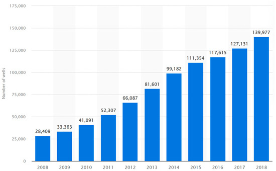
Figure 1.
Increasing horizontal wells in the United States [9].

Table 1.
Shale plays and horizontal well parameters [10].
Table 2.
Average lateral length and number of stages of shale basins in the study [11].
Table 3.
Selected parameters of fracturing fluids in shale basins (source: Enverus Prism).
2.2. Multistage Fracturing
McCormick Oil Company and Halliburton Services, joined by national and international oil companies, conducted the first fracturing horizontal well “experiment” in a joint field project, demonstrating the integration possibility of fracturing to other well techniques and enhancing the comprehension of fracturing horizontal wells [12]. M.Y. Soliman and his colleagues in Halliburton innovated the multistage fracturing technique for horizontal wells, first reported in the SPE Forum in 1987 and published in 1990 [13], where they also discussed stress, fracture direction, conductivity, fracture, and well optimization, which explained the essential aspects of fracturing horizontal wells. Athabasca Oil Corporation conducted a microseismic trial with one on-azimuth and one 45° off-azimuth in the Duvernay Formation, as shown in the microseismic map of Figure 2b (fracture stages are depicted in multiple colors) [14].
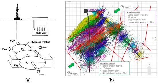
Figure 2.
Horizontal well multistage transverse fracture diagram (a) [13] and microseismic stage events for different azimuth horizontal wells (b) [14].
As Soliman et al. [12,15,16] indicated, the fracturing of horizontal wells is superior to vertical wells under the following conditions: (1) vertical restricted flows and nonideal formation productivity because of low permeability or shale streaks; (2) directions of natural fractures varying from that of stimulated fractures; (3) poor stress contrast between the pay zone and surrounding barriers. Based on the azimuth between the wellbore and horizontal stress, transverse and longitudinal are the two primary fracture directions, and the most preferred fracturing azimuth of the horizontal well is perpendicular to the minimum horizontal stress with multistage fracture planes intersecting along most laterals with a maximizing contact surface flow area and stimulated reservoir volume (SRV) (Figure 2a). Operators aim to maximize the fluid and proppant volume delivered within a relatively short time. Multiple clusters of stages are perforated and stimulated sequentially as the typical horizontal well completion. Reorientation will happen if the fractures deviate with horizontal stresses, and careless operational calculations would cause seriously rough sand faces, especially in transverse fractures [12,15]. Several critical questions, as Soliman and Grieser [16] mentioned, about multistage transverse fracturing wells are the optimum spacing, the well orientation with horizontal wells, the open area between fractures, and the best well fracturing timing. The optimum spacing is dependent on the fluid flow, stress interference, and economic costs. As Figure 3a shows, the simulated cumulative production increasing rate will decrease when the transverse fracture number increases, and after a certain number, increasing the number of fractures is not profitable anymore. Shelley and Soliman [17] simulated the effect of fracturing time for a gas–condensate reservoir where condensate banks can hinder fluid flow. A later fracturing time causes the formation of a larger condensate bank, which would cause a significant delay in gas production and lead to more uncoverable condensate (Figure 3b).
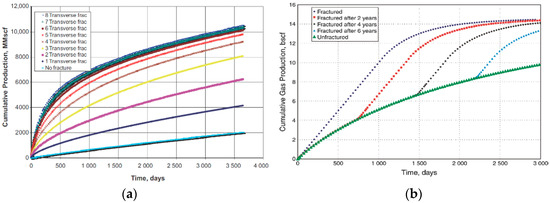
Figure 3.
The effect of the number of transverse fractures on productivity (a) [16] and fracturing time effect on gas–condensate reservoirs (b) [17].
2.3. Multistage Fracturing Mechanics
Applying Hubert and Willis’ failure criterion [18] of axial fracture tensile breakdown theory to longitudinal fracturing horizontal wells, the breakdown pressure can be expressed as Equation (1). After several laboratory observations, Huber and Willis’s theory was found unsuitable for transverse fractures of horizontal wells. Thus, Hoek and Brown’s shear failure criterion [19] was applied to transverse fracture breakdown pressure calculations expressed in Equation (2) [20,21]:
where —the breakdown pressure, —minimum horizontal stress, —maximum horizontal stress, —vertical stress, —the largest of and , —the smallest of and , and —the compressive strength of the rock. Figure 4a shows the treating pressure variation with horizontal trajectory angles associated with maximum horizontal stress, which shows it is easier to initiate longitudinal fractures than transverse fractures. Furthermore, fractures are prone to form at both edges of an open hole or along the perforated interval, resulting in complex T-shaped and I-beam fractures. To alleviate the complex fracture issue, the perforated interval should be controlled at less than four times the well diameter [21].
If initiated fractures are placed at an angle relative to the wellbore, they will reorient automatically to be perpendicular to the minimum horizontal stress and lead to abnormal pressure and premature sandout conditions. According to Deimbacher et al. [22], reorientation will cause a reduction in fracture width, and a general equation describing this reduction for an angle between the well and fracture was derived as
where is the well diameter, is the perforated interval, is the longitudinal fracture width, and is transverse fracture width. El-Rabaa and Rogiers in 1990 [23] considered both relative stress and fracture size and derived a more comprehensive equation [20,21].
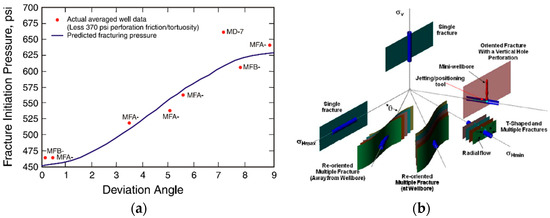
Figure 4.
Fracture initial pressure at different trajectory angle horizontal wells with maximum horizontal stress in the Dan Field (a) [21,24,25] and different fracture geometries of well orientations with an in situ stress field (b) [15].
Figure 4.
Fracture initial pressure at different trajectory angle horizontal wells with maximum horizontal stress in the Dan Field (a) [21,24,25] and different fracture geometries of well orientations with an in situ stress field (b) [15].

The fracture usually propagates in a tensile mode (mode I), sliding mode (mode II), and tearing mode (mode III) with the assumption of linear elastic fracture mechanics (LEFM) in an isotropic medium. The fracture propagation should satisfy the condition with stress intensity factors and of the tensile and sliding modes, fracture toughness , and fracture propagation angle [26]:
Increasing fluid pressure will only affect the tensile mode and push fractures to propagate aligning their orientation. In Figure 5a, the minimum horizontal stress is in the north–south direction, and fractures with higher internal fluid pressure are prone to reorient more reluctantly to theperpendicular direction. Other plots in Figure 5 show that fractures with a lower injection pressure, larger stress anisotropy, and larger drilled inclined angle will reorient more easily.
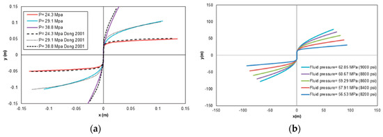
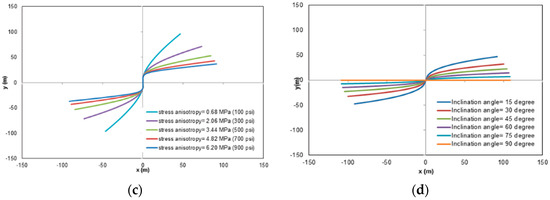
Figure 5.
Different fluid pressure (a), differential fluid pressure with a constant stress anisotropy (b), constant fluid pressure with different remote stress conditions (c), and fractures inclined at different angles (d) [26].
2.4. Conventional Multistage Fracture Completion Techniques
Over the past several decades, many innovative completion techniques focusing on the multistage fracturing of horizontal wells have been invented for open-hole, cased, and cemented completions to be compatible with different underground geological and geomechanical conditions and production objectives and schemes. In this section, several widely field-used conventional completion techniques are briefly summarized for description and comparison based on an elaborate study by Soliman et al. [12,27]. In cased and cemented completions, the most common method is the “limited-entry, cluster perforating and pump-down plug diversion method” (Perf and Plug), shown in Figure 6a, which has been successfully extensively applied in Barnett Shale in North Texas. After initial treatment with the coiled tubing system, each cluster from the individual stage is perforated by the explosive gun and isolated by composite bridge plugs from the toe toward the heel, and then the frac fluid is perforated into intervals. The process is repeated for each stage, and the plugs are milled out at the end of the treatment process. Although this method is comparably efficient, related issues such as premature screenout and the plug setting and uneven proppant distribution can cause low production efficiency. The nonideal efficiency can be remedied by an advanced technique known as “pinpoint stimulation”, by treating a single cluster per time with hydrajet perforating for constant and repeatable fracture sizes in each stage [28,29]. A newer open-hole method called the “ball activated sliding sleeve method” (BASS) in Figure 6b was developed to speed up multistage fracturing treatment by dropping incrementally larger balls to open frac sleeves in series to divert frac fluids within a single nonceasing pumping operation. Comparing the Perf and Plug method, the total perforating time decreased from 40 to 3 h [27], and the required completion time decreased within 50% to 70% [30]. In addition to the multistage completion mentioned above, the cased hole CT straddle-packer completion, compatible with energized or foamed fluids, deploys pre-perforation to decrease nonprolific time to improve efficiency and is more suitable for ductile reservoirs (Figure 7a). The ever-evolving hydrajet-assisted fracturing method, with the aid of hydrajetting energy, is extensively used in different completions without physical isolation equipment in a dynamic tubing movement (Figure 7b).
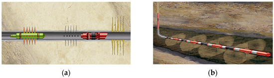
Figure 6.
Perf and Plug completion scheme (a) and BASS completion scheme (b) [27].
Figure 7.
CT straddle-packer completion (a) and hydrajet assisted fracturing completion (b) [27].
2.5. Multistage Horizontal Completion Innovations and Optimizations
Several authors have developed methods to manipulate the fracturing sequence to enhance the fracture complexity and the stimulated reservoir volume to improve hydraulic fracturing performance. In order to induce and enhance the fracture complexity in brittle far-field shale reservoirs, Soliman et al. [31,32] put forward two alternative completion options, especially for coiled tubing completed horizontal wells from 2010. The first approach, shown in Figure 8a, is named “Commuter Frac” (Stress-Diversion Method), with the novelty of integrating alternative pumping schedules with real-time net pressure and microseismic fracturing mapping (MSFM) for decision-making improvement. Targeting at exceeding the abrasive fluid pumping rate limit and alternative treatment fluid properties, this new method is aided with a high-rate nonabrasive fluid injection in the annulus to deliver the proppant in the coiled tubing (CT) to form branch fracturing deep in reservoirs with proppant bridging and pack at perforations by decreasing the pumping rate of slickwater. Overflush can be achieved by simply ceasing pumping in the CT. The second alternative method was termed as “Texas Two-Step”, which is a three-interval treatment from toe to heel with limited-entry perforations (Figure 8b). The stress field is altered between two main bi-wing fractures with natural fractures opened by higher net pressure, and then the third fracture is cracked with an inhibited length to connect parallel induced stress-relief fractures with bi-wing fractures. This alternative technique can be fulfilled by the mechanical shifting of sleeves (MSS) using coiled tubing or jointed pipe, which is compatible with the Commuter Frac method and enhances its performance enormously. As the authors demonstrated in the paper, the Commuter Frac method has been applied in Eagle Ford Shale in South Texas to solve the issues of Perf and Plug for a more aggressive and tailorable treatment schedule.
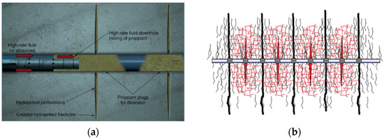
Figure 8.
Commuter Frac (a) and Texas Two-Step (b) alternative fracture completions [32].
Simultaneous and sequential hydraulic fracturing are popular and widely accepted by the industry with a fracture complexity design for broader fracture contacts. The propagation of fractures depends on the opposite fracture-tip stress perturbation to force the fractures to propagate perpendicular to the horizontal wells. To imitate the induced stress of the “Texas Two-Step” method, Rafiee et al. [33] proposed a new simplified alternative design named “Modified Zipper Frac” (MZF) (Figure 9) for the multistage laterals to further optimize the zipper frac with a staggered pattern and no downhole operations by changing the stress perturbation field with the middle fracture for every two consecutive fractures. After studying the stress interference of penny-shaped, semi-infinite, and elliptical fractures, they concluded that the minimum horizontal stress change is highest and serves as an indicator for stress anisotropy and fracture complexity variations, and its change becomes negligible for a length–height ratio larger than 5. As Figure 10 shows, the Modified Zipper Frac method can enhance production performance by increasing the far-field fracture network complexity.
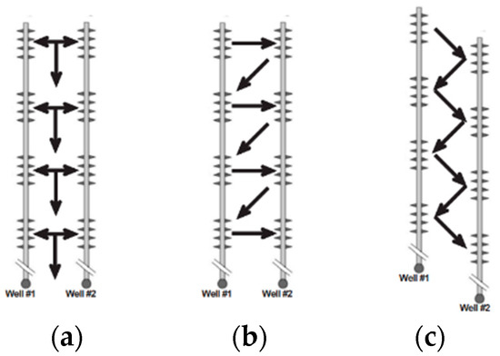
Figure 9.
Multiple horizontal well completion schemes (a)—simultaneous hydraulic fracturing; (b)—sequential fracturing (Zipper Frac); (c)—Modified Zipper Frac [34].
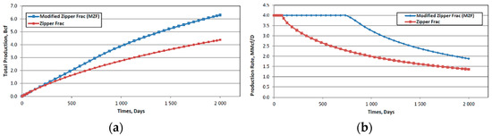
Figure 10.
Total production (a) and production rate (b) of Zipper Frac and Modified Zipper Frac scheme comparison [33].
In order to restrain the water-channeling issues in water-injection scenarios with an adverse recovery efficiency, Sierra et al. [35] came up with a new completion methodology for transverse horizontal production wells, which considers placing nonconductive fracture barrier fractures (NCBFs) sequentially at the horizontal production wells to modify the water front, delay water intrusion, and improve water-sweep area, as shown in Figure 11a. This technique can be applied during any phase of the open-hole completion process using the modified hydrajet-assisted fracturing completion and provides a more flexible design for water-injection projects with inflow-control devices (ICDs) and inflow-control valves (ICVs). The optimum option for the injection well is a vertical well, and the horizontal injection well and partial injection with partial production of one horizontal well schemes can also be considered. This methodology is more cost-efficient regarding produced water disposal, which can alsopotentially applied to other EOR scenarios.
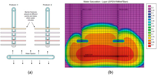
Figure 11.
Multiple barrier fracture diagram (a) and simulated water saturation area profiles of a field study in Saudi Arabia (b) [35].
2.6. Typical Multistage Fracture Treatment Parameters
Hydraulic fracturing fluids are generally a combination of base fluids, additives, and proppants. The fracturing fluids are injected at a high-enough rate to surpass the breakdown pressure to initiate and propagate the fractures and carry and transport proppants to prop the fractures. The fracturing fluids should possess characteristics such as compatibility, stability, breakability, mixability, and cost and environmental friendliness. Among all the fracturing fluids, slickwater is most commonly used in the industry, mixing water-based fluids and friction-reducing additives. Low-viscosity slickwater generates less width but much longer fractures, increasing the far-field fracture complexity. The approximate basic slickwater composition for shale formations is expressed in terms of total volume: 98 to 99% water, 1 to 1.9% proppant (sand or ceramic particles), 0.025% friction reducer (polyacrylamide), 0.005 to 0.05% disinfectant (biocide), 0.05 to 0.2% surfactants, 0.2 to 0.5% corrosion inhibitor, gelation chemicals (guar gum, cellulose polymers), scale inhibitors (phosphate esters or phosphonates), and hydrochloric acid [36,37]. According to their functions, the fracturing fluid additives can be categorized into the gelling agent, friction reducer, breaker, crosslinker, and iron control. Table 4 and Table 5 summarize the fracturing fluids into the fluid type, main composition, and pros and cons. The fracture proppants initially were sand (Ottawa, Jordan, Hickory, etc.) and ceramic (HYDROPROP, ECONOPROP, CARBOLITE, etc.). Other materials have been developed for improved properties, such as resin-coated sands, ceramic-coated sands, and sintered bauxite [38]. Typical costs of different proppant types are depicted in Figure 12.
Table 4.
Fracturing fluids and chemicals (adapted from Gandossi [39]).
Table 4.
Fracturing fluids and chemicals (adapted from Gandossi [39]).
| Base Fluid | Fluid Type | Main Composition |
|---|---|---|
| Water-based | Slickwater | Water + sand (+ chemical additives) |
| Linear fluids | Gelled water, GUAR < HPG, HEC, CMHPG | |
| Crosslinked fluids | Crosslinker + GUAR, HPG, CMHPG, CMHEC | |
| Viscoelastic surfactant gel fluids | Electrolite + surfactant | |
| Foam-based | Water-based foam | Water and foamer + N2 or CO2 |
| Acid-based foam | Acid and foamer + N2 | |
| Alcohol-based foam | Methanol and foamer + N2 | |
| Oil-based | Linear fluids | Oil, gelled oil |
| Crosslinked fluids | Phosphate ester gels | |
| Water Emulsion | Water + oil + emulsifiers | |
| Acid-based | Linear fluids | - |
| Crosslinked fluids | - | |
| Oil Emulsion | - | |
| Alcohol-based | Methanol/water mixes or 100% methanol | Methanol + water |
| Emulsion-based | Water–oil emulsions | Water + oil |
| CO2–methanol | CO2 + water + methanol | |
| Others | - | |
| Other fluids | Liquid CO2 | CO2 |
| Liquid nitrogen | N2 | |
| Liquid helium | He | |
| Liquid natural gas | LPG (butane and propane) |
Table 5.
The summary of different fracturing fluids (summarized from Gandossi [39]).
Table 5.
The summary of different fracturing fluids (summarized from Gandossi [39]).
| Base Fluid | Pros and Cons |
|---|---|
| Water-based | Most cost-effective and available, incombustible, simplest viscosity control. Not suitable for water-sensitive formation, water trapping, less capability of proppant transport of slickwater |
| Foam-based | Reduction in water usage, additives, and formation damage; better residual cleanup; high viscosity and proppant transport capability. High costs, rheological uncertainty, and the need for higher pumping rates |
| Oil-based | Compatible with almost any formation type. Potential high cost and concerns with safety and environmental effects |
| Acid-based | Needs continuous carbonate/limestone phases to etch, and disposal of solutes, short fractures due to high leakoff and rapid acid reaction |
| Alcohol-based | Potential to decrease water trapping, compatible with water-sensitive formations, and stabilizes temperature. Flammable, expensive, extra spending with personnel training, easy to degrade |
| Emulsion-based | Similar to foam-based fluids and depends on oil or water external emulsion |
| Other fluids | Provide substantial energy to recover fluids, which is suitable for low bottom-hole pressure formations, and less water to alleviate damage to water-sensitive formations; reduce the proppant amount, high costs |
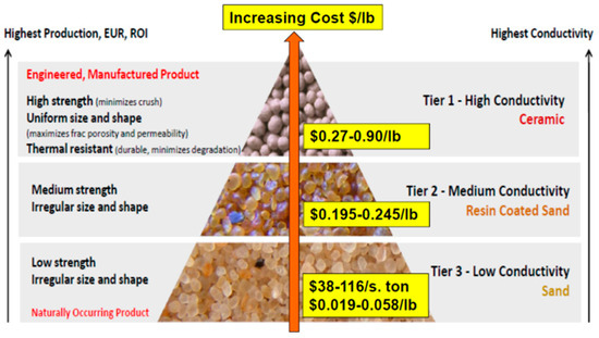
Figure 12.
The typical costs of proppants in different types (source: P&L International Trading) [40].
Figure 12.
The typical costs of proppants in different types (source: P&L International Trading) [40].

Selected actual field data can provide a shared sense of treatment ranges. According to project team experience, in conventional fracturing, “the fracture pressure gradient is typically 0.4–1.2 psi/foot (0.09–0.27 bar/meter). The fluid pressures used in high-volume hydraulic fracturing are typically 10,000 to 15,000 psi (700–1000 bar) and exceptionally up to 20,000 psi (1400 bar), which compares to a pressure of up to 10,000 psi (700 bar) for a conventional well. In the tight-gas example from the Danish authorities, pressures of up to 8400 psi (580 bar) were applied [36]. Another real field example is the several horizontal wells, completed in sequence with preplanned fracture and reservoir diagnostics, of Marcellus Shale by Seneca Resources in Houston, Texas [41]. Two transverse-fractured horizontal wells with Plug and Perf completions were perforated at 2500 feet and 2300 feet. “Both wells were fracture stimulated with seven-stage fracture completions at pump rates of 80–95 barrels a minute. Each frac stage consisted of pumping 350,000 gallons (8350 barrels) of a slickwater fluid system, with 56,000 pounds of 100-mesh sand, 110,000 pounds of 40/70-mesh Jordan sand, and 270,000 pounds of 30/50-mesh Jordan sand”. East et al. [42], focusing on hydrajet fracturing, presented a comparison of varied completion techniques. A summary of the completion parameters for the case-history wells in Barnett Shale is provided in Table 1 and Table 2 of this paper for more reference, including completion and treatment type, total treatment volume and total sand in treatment, and typical average rates.
3. Fracture Modeling and Simulation
3.1. Fracture Propagation Modeling
Since the 1950s, several groundbreaking theoretical fracture models have been developed for different dimensions under several related assumptions. The predominant 2D fracture models are the Khristianovic–Geertsma–de Klerk (KGD) model and the Perkins–Kern–Nordgren (PKN) model under the presumption of a plain strain and penny-shaped crack model of the line source. The pseudo 3D and planar 3D fracture models are broadly applied to simulate the fracture propagation and closure period to remedy the variable fracture height decreasing from the wellbore. Compared to the full 3D model, the pseudo 3D model decreases the calculation complexity and is better for routine designs. As Figure 13 shows, Adachi et al. [43] summarized and compared different dimensional propagation models and their flow mechanisms. This section discusses the fracture propagation process regarding fluid flow, material balance, and other geomechanical aspects.
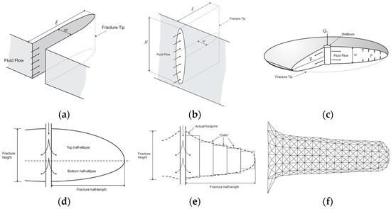
Figure 13.
Typical propagation models: KGD model (a), PKN model (b), radial model (c), lumped elliptical model (d), cell-based model (e), and planar 3D model (f) [43].
Material balance equations serve as the governing equations for planar fracture propagation continuity. The sequential equations below are the general form of material balance equations where all terms are expressed in three dimensions. The Newtonian and power-law fluid flow and leakoff equations can be expressed in two dimensions [43]:
where —fracture width, —time, exposure time, —fluid pressure inside the fracture, —fluid density, g—gravity vector, —source injection rate, —Carter leakoff coefficient, power-law exponent, consistency index, gravity vector components, Dirac delta function, the spurt loss. For the Newtonian fluid, = 1, , then , viscosity.
Based on a coupled finite-volume (FV)/finite-area (FA) model, Manchanda et al. [44] summarized the governing equations and brought up the numerical model algorithm for multiple fracture propagation simulations with the integration of reservoir geomechanics. Their proposed method has been testified with analytical solutions and field data as a comprehensive three-dimensional hydraulic fracture modeling at the pad scale. As shown in Figure 14, using the resistance calculation with pressure drops in the wellbore, perforations, and injection points, the slurry distribution can be calculated [44]:
where resistance of ith cluster, injection rate of each cluster, ith cluster pressure at injection point, wellbore pressure, and perforation pressure difference.
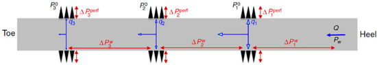
Figure 14.
Flow distribution between multiple clusters [44].
Several advanced hydraulic fracture propagation modeling technologies have developed over time. Distributed fiber-optic sensing (DFOS) techniques have been applied in hydraulic fracture characterization and calibration in unconventional reservoirs for fracturing propagation and geometry observation in the near- and far-field over the past two decades since the first DFOs were installed in 1993 [45], which generally are categorized into distributed acoustic sensing (DAS) (Figure 15 and Figure 16a) and distributed temperature sensing (DTS) (Figure 16b). Usually, a permanent fiber-optic-cable system is placed and cemented externally on the monitor wellbore casing or through wirelines to obtain DAS and DTS measurements for clusters and stage efficiency [46,47]. DTS and DAS can be applied to interpret wellbore, near-wellbore and far-field regions. DTS technology is a sensitive measurement that captures the temperature change with time and space during stimulation when fluids enter formation via clusters. At the same time, high-resolution DAS can be utilized for the low-frequency strain variation in offset fracture interactions during the stimulation deformation period. One promising field example in 2013 was when Pioneer Natural Resources Company applied DFOS in a 10,000-foot horizontal well of Wolfcamp Shale of Midland County equipped with downhole pressure gauges and microseismic geophones. The monitor vertical well and adjacent offsetting horizontal wells were stimulated in a Zipper Frac sequence for measurements and delineation of near- and far-field well and formation interactions [48]. Frac hit corridor (FHC) is a relatively new processing method for hydraulic fracture evaluation of the far-field strain (FFS) monitor model. As Figure 15 and Figure 16a show, the tension in reading is generated hugely before the fracture tip, along with compression in blue as the hydraulic fracture propagation. When frac tips near the monitor well, a distinct red tension region occurs, and when frac tips pass by the monitor well, the blue compression region shows above and below the tension region. The stress flipping at the final time indicates the fracture closure. In Figure 17, two multistage fractured horizontal wells were developed from zipper fracking completion and monitored by another horizontal well.
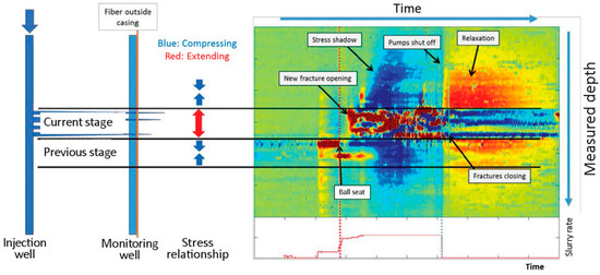
Figure 15.
Low-frequency DAS stress response plot during hydraulic fracturing [49].
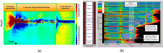
Figure 16.
Tension and compression variations of DAS in the hydraulic fracturing process (a) [50] and DTS colormap for seven stages (b) [51].
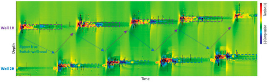
Figure 17.
Multistage Zipper Frac FFS plot (FHC represented by dotted line rectangles) [46].
In contrast to the variable fracture models mentioned above, which focus on the propagation process, specializing the multifractured horizontal wells in a limited aspect of fracturing, several researchers have concentrated only on developing versatile and flexible analytical solutions in steps for the pressure and flow behavior and distribution of pre-existing fractures with stimulated regions in shale reservoirs. In many real cases, combined with the reservoir fracture network, the propped branched fracture geometry is far more complicated than the conventional and straightforward bi-wing shape (Figure 18). For simulation simplification purposes, these branched fractures always are approximated with a transverse bi-wing shape fracture with a higher-permeability rectangular stimulated region (SRV) around the fracture. Brown et al. [52,53] 2011 first proposed the trilinear flow model (TLF) to find a practical analytical solution associated with flow regime parameter calculations as a complementary method of previous semi-analytical and numerical simulations, with the merit of fewer data needs and computation time. As Figure 19a shows, the TLF model couples no-flow boundaries with three contiguously one-directional linear flows of single-phase and constant compressible fluids in the outer reservoir beyond tips, inner-stimulated reservoir regions between fractures, and hydraulic fractures. Later, Stalgorova and Mattar [54] in 2012 presented an enhanced-fracture-region (EFR) model (Figure 19b) by varying the TLF model geometry with limited areas around fractures and removing unstimulated regions beyond tips because of the extremely low permeability. In one-quarter of a fracture, three one-dimensional linear flows are applied as the fracture flow toward the well, the stimulated-region flow toward the fracture, and the unstimulated-region flow toward the stimulated region. Sequentially, by integrating the TLF model and EFR model, considering the long-term production contribution of unstimulated regions beyond tips, a more complex extended five-region model [55] was brought up and warranted by the reasonable agreement with numerical results for alternative configuration satisfaction (Figure 19c). The analytical solutions of the three previous models all require placing the fracture symmetrically in the fracture-stimulated unit, which is not flexible and rigorous enough to capture all the production configurations where fractures are not equally spaced. Heidari Sureshjani and Clarkson [56] presented an improved EFR model with asymmetrical lateral spacing to remedy this deficiency. Moreover, this new method also substitutes the two-dimensional flow with a one-dimensional flow in the unstimulated region of the well direction for more realistic conditions.
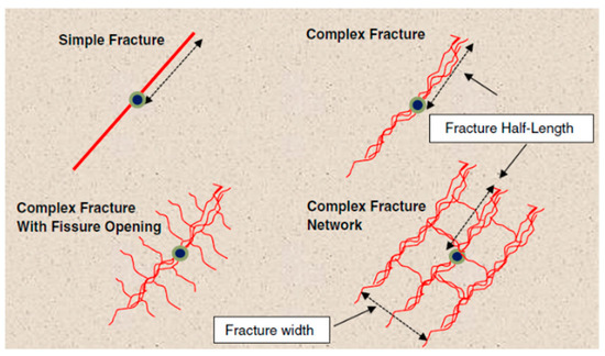
Figure 18.
Expected fracture geometry diagrams for fractured reservoirs [57].
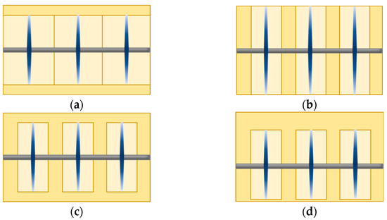
Figure 19.
Trilinear-flow model (a), enhanced-fracture-region model (b), five-region model (c) and asymmetric enhanced-fracture-region model (d) (modified from Stalgorova et al. [55] and Heidari Sureshjani et al. [56]).
3.2. Fracturing Flowback
In the hydraulic fracturing process, a considerable amount of fracturing fluids are usually pumped at high pressure into formations; however, most of them are probably imbibed or trapped in the natural fractures, and only 10–40% of fracturing fluids are recovered [58]. Researchers are trying to figure out the distribution of unrecovered fracturing fluids and the use of flowback data analysis. Clarkson [57] discusses rate transient analysis (RTA), similar to PTA (pressure transient analysis), for unconventional gas reservoirs, viz. shale gas, tight gas, and coalbed methane. RTA is related to quantitative production data analysis (PDA) and consists of using reservoir models for obtaining basic reservoir information such as hydrocarbon in place, permeability, and skin factor to make a prediction of pressure and rate. Inspired by the previous flowback studies from Crafton et al. [59,60,61,62,63], a detailed workflow has been presented for the data analysis procedure from Clarkson et al. [64,65,66], which was initially designed for online production data analysis. However, it has been adopted for flowback RTA of MFHWs completed in unconventional formations, which is superior to decline curve analysis, which is an empirical method. Most RTA calculations have focused on long-term production, and previous studies also showed that a short-term (often in hours) flowback period, happening immediately after fracture propagation treatment (Figure 20), can also be applied to the same analysis procedures for a possible flow regime to timely estimate hydraulic fracture properties to future fracture stimulation treatment designs and operational strategies. As Figure 21 and Figure 22 show, in the early flowback period, the intrafracture transient linear flow (IFTLF) and intrafracture boundary-dominated flow (IFBDF) in the log-log coordinates are generally expected to show in the early flowback period. Compared to the online production period, the quantitative analysis of flowback requires more frequent data acquisition and values on fracture/reservoir fluids, intrafracture flows, and fracture geomechanics [67].
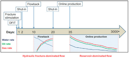
Figure 20.
The typical operation sequence of MFHWs [65,67].
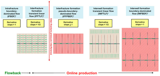
Figure 21.
Conceptual flow regimes of MFHWs in shale reservoirs. * Introduced terminology by Clarkson et al. [65].

Figure 22.
Flowback IRNP/IRNP’ analysis of Montney and Duvernay study wells [65,66].
Due to leakoff, unlike the online production using original reservoir conditions as the initial conditions, the initial conditions are altered during the flowback period. Thus, based on dynamic-drainage-area (DDA) concepts, Clarkson et al. [67,68,69] demonstrated the semi-analytical models for initial condition estimation with a primary hydraulic fracture (PHF) for hydrocarbon and water production in early time. Later, a method of water and gas production and pressure analysis in flowback of shale gas wells was presented with Marcellus Shale field examples for the first time [70]. In other work, Clarkson et al. [71] indicated that the flowback of multifractured horizontal wells often starts with a short single-phase flow of fracture storage used for fracture permeability and half-length calculation before the breakthrough. After the hydrocarbon breakthrough, there will be a multiphase flow in the fracture and linear flow from formation to fracture. Within these periods, the stress variation can cause fracture closure with different degrees of conductivity loss The conceptual models are given in Figure 23. With similar model concepts, Alkouh et al. [72] developed a 3D gas/water flowback simulator to simulate and calculate the effective fracture volume based on combined (flowback and production) data with a modified total compressibility by using water-rate-normalized pressure analysis. The authors demonstrated two field examples from the Fayetteville and Barnett formations to test the developed method. Fu et al. [73] developed a diagnostic six-step methodology for understanding flowback rate and pressure behavior. The steps include the model for estimating the effective fracture pore volume with early flowback data by RTA analysis, the estimation of fracture compressibility from DFIT data, a Pearson correlation coefficient to compare the effective fracture volume with the completion design parameters, etc., and multifractured horizontal well data from Woodford Shale of Anadarko Basin were used to testify the theory.
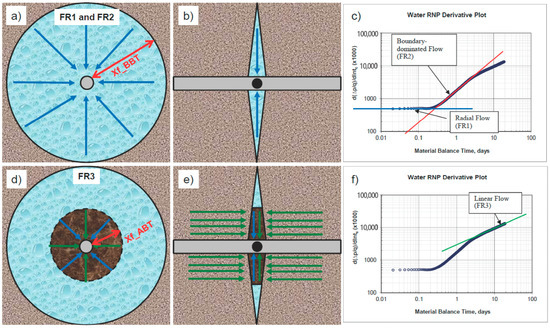
Figure 23.
Flowback model and RTA proposed by Clarkson et al. Cross-section view (a) and plan view (b) of a fracture with transient radial (FR1) and boundary-dominated water flow (FR2), which are reflected in the rate-normalized pressure derivative before breakthrough (BBT) (c). Transient linear oil flow from formation in cross-section view (d) and plan view (e), expressed with rate-normalized pressure derivative after breakthrough (ABT) (f) [71].
Another predominant topic of the flowback period is the salinity issues of hydraulic fracturing fluids, which cause environmental containment and production impact concerns. Figure 24 depicts the flowback water salinity of different U.S. shales in 2011, expressed in the concentration of total suspended solids (TDS). The flowback fluids can obtain a lot of salts from several mechanisms like the dissolution of minerals, bound water, and fracturing fluid interaction, which can sometimes reach up to 300,000 mg/L [74]. Zeng et al. [74] conducted spontaneous imbibition experiments using deionized water and outcrops from the Marcellus, Barnett, and Eagle Ford Shales by monitoring the pH, electrical conductivity, and ion concentrations of the surrounding water. Their geochemical modeling showed that the frac fluid and shale interactions (mineral dissolution, surface complexation) are less than 3% with minor impact, suggesting that fluid interactions caused high salinity.
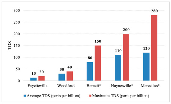
Figure 24.
Flowback water salinity of U.S. Shales (modified from Statista). * Potential higher Maxima than the listed numbers [75].
3.3. Commercial Software Simulators
The numerical methods, such as continuum-based methods (BEM, FEM, XEFM, FDM, etc.) and the discontinuum-based methods (DEM, RBSN, peridynamics, etc.), have been extensively developed and applied in hydraulic fracturing simulations for various specific questions. Based on these basic numerical methods, the Dynardo simulator combines ANSYS, multiPlas, and optiSlang for the hydraulic fracturing process, where ANSYS is used for parametric reservoir finite element models with hydraulic–mechanical analysis, multiPlus is the nonlinear material modeling ANSYS extension of fractured rock, and optiSlang is applied for efficient calibration and sensitive analysis [76].
However, these numerical methods require time-consuming mathematical capability, and therefore, based on these theories, commercial simulators arose and gained popularity for their advanced efficiency, accuracy, comprehension of geology, geomechanics, and reservoir production [77]. It should be noted that most high-tech companies used different modeling methodologies and function achievements to develop the planar 3D simulators; as a result, commercial simulators are not universal and produce output with disparate fracture geometries under the same initial conditions [78]. Soliman and Grieser [16] indicated that a good simulator should follow a design philosophy: (1) emphasize production-related predictions for a single well or a small group of wells; (2) use a graphical interface to provide a high efficiency of simulation and turnarounds; (3) simulate crucial features automatically, such as fracturing fluid filtrates, proppant library linkage, and fracture geometries; (4) create a grid system to reflect the flow regime in fractures accurately; (5) allow performance-affecting inputs; and (6) provide over-time postprocessing 2D and 3D plots or animations for flow demonstration. This section first includes a general summary of different commercial simulators (Table 6), then focuses on brief descriptions of several popular ones.
Table 6.
Commercially popular hydraulic fracture software (modified from Chen et al. [77] and Dobbs et al. [78]). Note: multiple HFs include leakoff and proppant transport; HF—hydraulic fracture, UFM—unconventional fracture model, MS—microseismic events, DFN—discrete fracture network, P3D—pseudo 3D, PL3D—planar 3D, ✓ — achievable function.
ResFrac, backed by the Altira Group, is in rapid development and gaining popularity since its launch in 2018, and it has collaborated with more than 35 leading E&P companies. At every time step, ResFrac can solve all the equations with the same consistent mesh, and the objective is to integrate the fracture propagation, reservoir flow, and geomechanics to simulate the complete well life cycle with a single model at all reservoir conditions to provide a robust numerical accuracy for field application and maximize economic returns after optimization. A detailed theoretical description for model building is provided in their technical writeup [79], and a step-by-step instruction document [80] with training videos for beginners is provided for quick learning and use. The comparison cases simulated in ResFrac are shown in Figure 25. One of their recent field applications is combined with DAS techniques [50] in the Midland Basin, where Shahri et al. from Apache described the elaborate collaboration between ResFrac and DAS of Silixa from single fracture simulation comparisons of Young’s modulus, fracture wellbore intersection angle, fracture height, permeability, and viscosity to multiple-cluster simulation calibration, and frac corridors and two other cases were studied (Figure 26a). The calibration is via comparing the spatial stress and strain tensors produced by ResFrac with DAS strain data for modeling accuracy and optimization. ResFrac also performed a parent/child study project with ten datasets from Midland, Delaware, Bakken, and Montney for economic-performance-improving optimizations. Recently, Ratcliff et al. [81] conducted a modeling study of the fracture-driven interaction (FDI) (frac hits) damage impact between a parent and child well of the STACK play. They used several testing and monitoring methods to calibrate the propped length, production rates, and parent and child productivity and enabled ResFrac simulation to replicate the parent–child well productions effectively.
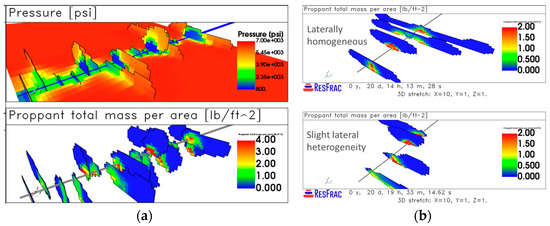
Figure 25.
Pressure and proppant distribution (a), homogeneous and lateral heterogeneity comparison (b) simulation by ResFrac [82].
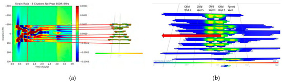
Figure 26.
Application with fiber-optic technology (a) [50] and parent/child study (b) of ResFrac [81].
GOHFER (the Grid-Oriented Hydraulic Fracture Extension Replicator) has been utilized for hydraulic fracture simulations in the industry for over 30 years since developed by Dr. Robert Barree of Barree & Associates LLC, who joined Halliburton later. Several of his early papers demonstrated the GOHFER capability to accurately model the fracture geometries during propagation with random spatial rock and fluid properties in heterogeneous media [83], the pressure profile of classic tip-screenout theory developed by Nolte and Smith [84], a rigorous study by stimulating the fracture flowback and proppant migration [85], falloff pressure and pressure derivatives of the G-function predicted by GOHFER [86], and a height-containment study of hydraulic fractures in laminated sand and shale sequences [87]. After decades of development, GOHFER was acquired by Halliburton and is now recognized as the chief and dominant comprehensive three-dimensional hydraulic fracture simulator in the industry with all petroleum-engineering-related disciplines. Halliburton provides several technical references for the theory and applications adopted in GOHFER for a quick check, which includes its general capability description [88], stress shadow of interference [89], fracture conductivity and clean-up [90], and their detailed user manual [91]. Zhan et al. [92] correlated pumping schedule data with reservoir performance by coupling GOHFER simulation output with a CMG geomechanics module as an integrated characterized method under the linear-elastic constitutive law and Barton–Bandis tensile model of shale gas reservoirs. Their work showed that the effective normal stress would increase as the shale gas reservoir develops with depleted porosity and permeability. Medina et al. [93] built a 3D geomechanical model for a shale reservoir discrete fracture network (DFN) (Figure 27a) and its hydraulic fracturing analysis. Within this model, based on the one-dimensional geomechanical model with a normal and strike slip, GOHFER was used for hydraulic fracturing stimulation with a slickwater and hybrid completion treatment in specific intervals.
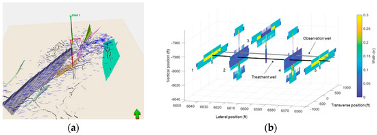
Figure 27.
Constructed DFN model plan view (a) [93] and five simulated fracture geometries for a DAS study with GOHFER at different temperature profiles (b) [94].
Another numerical simulator from Halliburton developed by Soliman et al. called “QuikLook” is compatible with advanced multiphase, four-component, nonisothermal, and three-dimensional simulation functions. The simulator is linked to WellCat™ wellbore simulator software and is capable of importing the generation results from StimPlan and GOHFER. The primary function of QuikLook is well-treatment optimization and design, which emphasizes fracturing and conformance. From the studies of Soliman et al. [16,95], it can also be utilized for the prediction of underbalanced drilling behavior, complex wells of reservoir production, sand control, and geomechanics effects. Conformance technologies control unwanted water and gas production. Ansah et al. [96] used QuikLook, coupling the wellbore and reservoir for design optimization and the efficiency evaluation of conformance decisions in water-coning and water-channeling cases, to help shorten the design process for the optimal conformance treatment of targeted wells.
Similarly, East et al. [97] used QuikLook to simulate and demonstrate the sweep profile alterations of the horizontal well during waterflooding. After-closure analysis can remediate the weakness of previous fracture diagnostic techniques. Soliman et al. [98] simulated the MiniFrac tests for both oil and gas reservoirs with aqueous phases injected as fracturing fluids. Guidelines were developed based on the analysis of numerically simulated fall-off data from QuikLook, which also helped to demonstrate the pressure profile at different mobility ratios (Figure 28a). Saputelli et al. [99] showed a design optimization of a multifractured 10,000-ft horizontal well in the Bakken Shale to help understand the effect of increasing fractures on economic incrementation, with the aid of the pseudo-compositional model of QuikLook showing that the open-hole provided a better performance (Figure 28b).
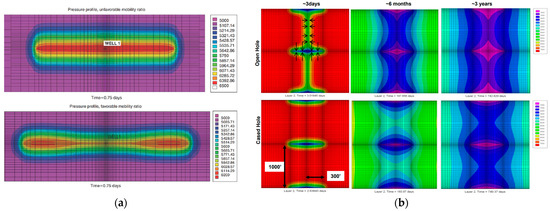
Figure 28.
Pressure profile of different mobility ratios (a) [98] and pressure maps for the open-hole and cased hole of the QuikLook simulation (b) [99].
4. Refracturing
When the production of horizontal wells continues decreasing, refracturing is the operational process that can be considered for the restimulation or completion of operational correctness after initial hydraulic fracturing production with altered stress fields, which will facilitate an improvement in connectivity with reservoirs and well productivity by bypassing the near-wellbore regions. Other advantages of refracturing techniques are to improve the ultimate recovery, modify the unequal contribution of induced fractures, and the subexecution of primary fractures [100]. Daneshy [100] also mentioned that the refracturing process with horizontal wells would be different from vertical wells because of the multistage completions, as well as the pressure reduction, total stress alteration, and different spacings, which will bring technical difficulties. Smith et al. [101] discussed the two-sided effects of pressure depletion on the refracturing process.
The isolation of different generations of fractures is also essential to avoid fluid–particle migration to previous fracture zones. The solid expandable tubulars [102,103], dynamic diversion techniques [104], biodegradable materials [105], and compression-set straddle packers [106] are methods applied for the isolations. The general refracturing method includes fluid injection to further extend and resurge the existing fractures or initiate new fractures. As Figure 29a shows, the unparallel paths of new fractures change due to the local principal stress orientation and magnitude after initial pressure depletion, and the deflection decreases as the distance from the initial fractures increases. Also, Figure 29b shows that during the refracturing process of pre-existing fractures, injection pressure variation can serve as an indicator to determine the fracture situation and slurry injection timing for the extension. In the early stage, the injection pressure increment will help widen fractures, and the injection pressure will decrease slightly when the fracture restarts extension afterward.
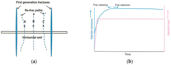
Figure 29.
Reservoir depletion effect on refracturing new fractures between transverse fractures (a) and pressure variation in refracturing existing fractures (b) [100].
Proper candidate selection is one significant part of the successful refracturing process. Horizontal wells with underperforming original fracturing, initial production below the economic limit, and other unfractured formations are good candidates for refracturing. The candidate selection process includes the early collection of reservoir engineering, drilling, and well-logging data with quality checks, followed by a multistage screening process and a more comprehensive diagnostic analysis [106]. Fragachan et al. [106] also demonstrated that the qualitative and quantitative analysis procedures for refracturing can be estimated by a quadrant plot, which compares the completion efficiency and reservoir quality. As Miller et al. [11] stated, only one-third of clusters were in effective production, and Plug and Perf completions have uneven distributions and fracture geometries with many unstimulated regions, which provide a high potential for refracturing. Wang et al. [107] performed a refracturing study in 2013 with data produced from 200 re-fractured wells of Barnett Shale with multiple analysis methods. As a representative DCA plot of a gas well production shown in Figure 30, refracturing can significantly enhance well performance.
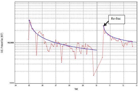
Figure 30.
Production decline curve analysis [107].
5. The Practice of Formation Fracturing
Miller et al. [11] interpreted more than 100 horizontal wells in shale plays from logs. The evaluation shows the high lateral variations, and almost one-third of clusters did not contribute to production. It was also demonstrated that only one-third of completion clusters contribute 50–60% of the total hydraulic fracturing production [30], which could be the consequence of the heterogenous issues of shale plays. Figure 31a shows the brittle and ductile rock variations in a 4000 ft lateral in Haynesville Shale [32]. Thus, the location and distribution of transverse fractures are very significant for production optimization, leading to the generation of the concept of the rock brittleness index (BI) to describe formations that are likely to have complex fracture networks, which combines Young’s modulus (E) and Poisson’s ratio (). Young’s modulus reflects the failure capacity, while Poisson’s ratio reflects the fracture support capability. Brittle rock has a large Young’s modulus and a low Poisson’s ratio. It is necessary to quantify the brittleness because ductile rocks yield to induced stress more easily, have more proppant embedment issues, and contain fewer microfractures, making them less than ideal candidates for hydraulic fracturing. As shown in Figure 31b, Rickman et al. first defined the brittleness index as the ratio of Young’s modulus and Poisson’s ratio and the brittle shale data located in the southwest part of the brittleness index plot. The fracturability index (FI) is another concept of sweet-spot identification for well and fracture placement. Alzahabi and Soliman [108,109,110] developed a new algorithm and optimization criterion called Cascade Fracturing Technology (Figure 32a) for fracture spacing to speed up production based on the FI by prioritizing the brittle and high in situ stress zones and considering the stress shadow along the laterals focusing on the productive segments of horizontal wells. Figure 32b shows their developed sweet-spot selection methodology for the placements of the well and fractures. Moreover, Mullen and Enderlin [111] proposed a complex fracturability index (CFI) method to qualitatively and quantitively categorize the formation-creating ability of fracture networks, which integrates the sedimentary fabric, stratigraphic properties, mineral distribution, and orientation of pre-existing planes of weakness techniques. Table 7 lists the typical brittleness index and fracturability index calculation methods based on previous studies’ mechanical properties, mineralogy, and failure criteria.

Figure 31.
The brittleness track of a horizontal lateral (brittle rock identified in red and ductile rock identified in green) (a) [32] and a cross plot of Young’s modulus and Poisson’s ratio show the brittleness percentage (b) [112].
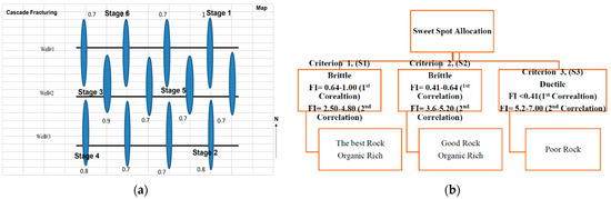
Figure 32.
Cascade Fracturing techniques (a) and a newly developed sweetspot identification methodology (b) for well and fracture location optimization [110].
Table 7.
Brief summary of brittleness index calculation and application (modified from Alzahabi [110], Li et al. [113], and Wood [114]). Note: BI—brittleness index, FI—fracturability Index, —normalized Young’s modulus, —the normalized Poisson’s ratio, —normalized brittleness, —strain energy release rate, —normalized fracture toughness, Q—quartz, C—carbonate, Cl—clay, Dol—dolomite, Lm—limestone, TOC—total organic content, —uniaxial compressive strength of rock, —tensile strength of rock.
Alzahabi et al. [110,123] also introduced a new sweet-spot identification method named mineralogical index maps to map productive shale more easily with attractive spots for effective transverse fracture locating. A mineralogical index value of 0.6 is a reasonable threshold to map the sweet spots. As demonstrated in Figure 33, the algorithm steps are analyzing data, building the mineralogical index and representative 3D model, formulating the problem, and optimizing the approach of well placement. Figure 34 shows a practical application of their optimization methodology consisting of 80 × 164 shale quality cells with two horizontal wells.
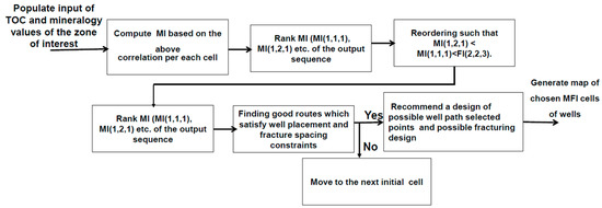
Figure 33.
Optimized well placement algorithm [123].

Figure 34.
A two-dimensional reservoir is divided into 80 × 80 equally sized cells in MATLAB, where the one-layer optimized well is in blue with fracture placements in red (b), based on the mineralogical index (MI) map with red-colored sweet-spot cells (a) [123].
6. Fracture Diagnostic Techniques
Fracture diagnostic techniques have been developed over decades. The normal diagnostics methods include Minifrac, DFIT, microseismic, fiber optic, and tiltmeter. The Nolte G- function [124,125,126] is essential for determining fracture closure pressure, rock properties, and leakoff calculation. The G-function, a dimensionless time function, connects the injection time () with the elapsed time () at a constant rate, which can be generally expressed as follows:
Conventional analysis DFIT methods are mainly applied to vertical wells because they are deficient in horizontal wells in unconventional reservoirs, which led researchers Eltaleb and Soliman [127] to apply the alternative signal processing approaches by decomposing different frequency fall-off nonstationary signals and analyzing the noise energy using a wavelet transform for closure identification. The most significant advantage of the wavelet transform method is that it does not depend on the fracture geometry and rock properties for broad and flexible applications in all kinds of fracture types. The signal energy represented by the closure period drops and keeps to a minimum level, testified to the authors’ hypothesis, and the closure time of the wavelet transform is different from the conventional G-function method. They demonstrated several field cases, and one case of DFIT showed that the G-function analysis could not precisely identify the closure time because of several plotted straight lines in a natural fracture system (Figure 35a); however, by using the wavelet transform method, the closure time could be determined by the intersection of energy regions A and B (Figure 35b).

Figure 35.
G-function plot (a) and the distribution of noise energy after the decomposition of the wavelet transform method (b) [127].
Eltaleb and Soliman [128] also applied the wavelet transform method with the heat exchange and fluid compressibility to a case study in the geothermal reservoir DFIT analyzation of the Utah FORGE formation by regarding the recorded pressure and temperature as the signal label of fracture closures. Compared to the wavelet transform method, the authors showed how G-function methods can underestimate the minimum horizontal stress and increasingly underestimate it after pressure correction in unconventional reservoirs. Awad and Soliman [129] applied the wavelet analysis to fracture propagation events for real-time fluid injection monitoring and early diagnosis with the advantage of the time localization of wavelet transform. The wavelet transform can also be applied for inferring interwell connectivity analysis [130].
7. Advances in Fracture Modeling
7.1. Black-Box Fast Multipole Method
Rezaei and Soliman [131] developed the black-box fast multipole method (bbFMM) for a variety of poroelastic fracture development situations, such as refracturing a horizontal well, infill fracturing in a depleted reservoir, etc. They compared bbFMM with several other methods for fracturing simulation based on the boundary element method (BEM). As an example of model application, Figure 36 shows the sequence of (a) perforating a horizontal well—there may be several perforations, but only one develops into (b) the initial fractures. After several years of production until reaching the limit threshold, (c) a depleted zone around hydraulic fractures with affected principal stresses forms around the fractures. (d) “Child” fractures form between the fractures, but ideal fracture propagation may not occur and will be determined by the time-dependent stress conditions. For different production period cases, the new fractures (child fractures) may bend toward the nearest initial fractures because of stress re-orientation, and this deviation degree increases as the time elapses, as shown in Figure 37. This situation happens as a result of a local maximum and minimum stress reversal. After a certain time for the complete stress reversal process, fracture propagation trajectories have no apparent changes. As shown in Figure 37, the complete stress reversal took almost three years to obtain stable fracture propagation paths.
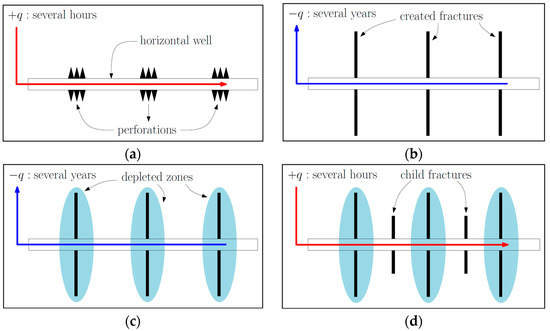
Figure 36.
Refracturing scheme: injection of high-pressure fluids into perforations (original fracture) (a); final length of the original fractures (b); depletion of the area around hydraulic fractures after production (c); creation of child fractures in the system after the decline in production (d) [131].

Figure 37.
Propagation of the new (child) fracture at different production times [131].
7.2. Progressive Nonintrusive Theory of Fracture Proppant Flow
In previous studies, the Eulerian–Eulerian method was applied to model the fluid–particle interactions with a relatively fast process, but it can raise a certain degree of inaccuracy in the physics when trying to upscale the solid properties. By combining the computational fluid dynamic (CFD) of fluids and the discrete element method (DEM) of particles, the Eulerian–Lagrangian method is highly accurate but computationally intensive and time-demanding to model fluid–solid flows. In order to balance accuracy and efficiency, based on smart domain decomposition (SDD), trajectory piecewise linearization (TPWL) and a referred 2D fluidized bed example in MFix, Razavi, Soliman, and Farouq Ali [132] developed a new verified universal theory to model solid–fluid reactions by characterizing the critical components as data points to build progressive nonintrusive methods (NIMs) to approximate the governing equations with solid behavior described by radial basis functions (RBFs) [133]. In the SDD process, a single snapshot reproduction by optimizing clustering with the representative centroid method can solve the dynamic solid domain problem, the first step to developing the whole theory. Within this process, 150 centroids were decreased to 6 centroids in an acceptable error range by sensitivity analysis to reduce the computational load. Next, as Figure 38 shows, the TPWL method using the linear combination of dynamics and gradients for the total system was utilized to connect the created single snapshot with pillar-serial and parallel bridges to a progressive NIM development with an explicit numerical scheme. It was also observed that the particles deviate from the expected path after several early movements by the collision of fluid–solid and solid–solid forces, which resulted in the authors proposing a two-step solution based on the K-dimensional tree (KD-tree) algorithm instead of parallel bridges.
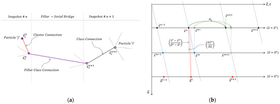
Figure 38.
Consecutive snapshot connection by the pillar-serial bridge (a) and the parallel bridge (b) [132].
A 2D solid fluidization bed called “gas blower” was applied to verify the proposed methodology. The advantages of the gas blower are that particles are constant numbers and move in all directions. As shown in Figure 39, the particles flow upward with gas and deposit with gravity during the transient period until they reach the equilibrium state of drag, collision, and gravity forces. As the snapshot of Figure 40 shows, the proposed methodology could accurately simulate and describe the fluid–particle movement with verification by MFix. It was also testified that the proposed nonintrusive approach can highly decrease the CPU running time by 8500 times and contains a higher than 95% accuracy, shown in Figure 41.
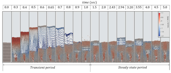
Figure 39.
The gas blower dynamic process from MFix runs for transient and steady-state periods [132].
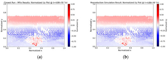
Figure 40.
The comparison of MFix results (a) and NIM results (b) [132].
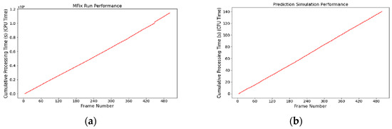
Figure 41.
Cumulative processing time of MFix runs (a) and NIM stimulations (b) [132].
7.3. Plasma Fracturing
Different from the massive water usage and certain degree of damage of chemical additives during the propagation of conventional hydraulic fracturing methods, the pulsed power plasma discharge (P3D) (or named electrohydraulic discharge) technique, as the extension of pulsed corona electrohydraulic discharge (PCED) or pulsed arc electrohydraulic discharge (PAED), is comparably cost-effective, repeatable, reliable, and an excellent candidate to eliminate these deficiencies by modifying the near-well region permeability with multiple self-propped short fractures [134]. Combined with electrical, mechanical, and electromagnetic processes, this technique extended with the thermite reaction of fusible metal links in water only requires water-filled wellbores, and it uses electrodes to discharge the fast plasma ions for generating pressure shockwaves to frac multiple micro- and macroscale fractures and generate electromagnetic fields [135,136]. A typical plasma pulse apparatus is shown in Figure 42. The purpose-built equipment in Figure 43 was also constructed for plasma fracturing purposes, which included the electrical devices, triaxial cell, and monitoring and recording system.
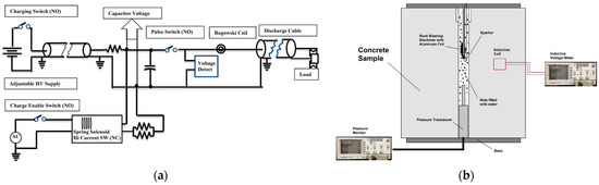
Figure 42.
General plasma pulse device (a) and the vertical view of sample placement (b) [134].

Figure 43.
Electrical components for storing and releasing electrical energy: the container cabinet (a), the capacitors and spark gap (b), the triaxial cell connected by the high voltage cables (c), electrodes and aluminum wire (d) [135].
Rezaei and Soliman [136] performed several tests to check the improvement of near-wellbore performance for cement, limestone, and sandstone samples and the enhancement of permeability and found that it could be achieved by inducing hair-like fractures and multiple discharges. Later, they [135] conducted four different open-hole plasma fracturing tests under triaxial stresses to investigate the effects of the fusible link, confining stress, discharge repetition, and the generated fracture characteristics with samples from outcrops in South Texas. Aluminum was chosen to be the fusible link for thermite reactions to study its effect. As shown in Figure 44, the experimental case used the aluminum wire to generate visible horizontal and vertical fractures, indicating that the thermite reaction can provide higher energy to frac the formations. Moreover, the differences in mechanical properties and heterogeneities like natural fracture distribution are also crucial for fracture initiation. Compared with sandstone, multiple fractures, including more shear fractures with less than a 90° angle, were observed in limestone, which indicates the pulsed plasma discharging techniques work better in heterogeneous shale reservoirs. The authors developed the energy needed for frac formation increases along the increment of confining stress and a relationship between discharge energy and confining stress with a shaded uncertainty allowance area, as shown in Figure 45a. Discharge repetition can help initiate new fractures and enlarge and elongate existing fractures. Five fractures in sequence due to the discharge repetition are shown in Figure 45b. The locations of induced fractures are indicated by the red arrows in Figure 44 and Figure 45.
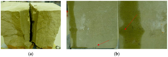
Figure 44.
Comparison of induced fractures in sandstone samples with aluminum wire (a) and without aluminum wire (b) [135].
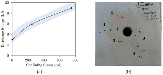
Figure 45.
Discharge energy and confining stress relationship with the uncertainty of limestone (a) and multifractures induced by discharge repetition (b) [135].
Xiao et al. [134] demonstrated various experiments with lab-scale cylindrical test samples to investigate this technique. PVC sleeves were used as the casing to prevent water penetration. They first performed four cement sample tests to mimic different wellbore completion cases. Then, a finite element model, as shown in Figure 46, was developed and verified by a near-wellbore laboratory zone to understand the electromagnetic behavior during the pulsed power plasma stimulation process. Furthermore, the conventional explosive perforation method can also lead to potential formation-plugging damage issues. Thus, the high-power plasma method is advantageous for effective hole perforation and fine particle removal. Bazargan et al. [137] also adopted the plasma torch in perforation and fracture initiation by proposing the finite element method (FEM) and performing experiments on plasma torch perforation. They also observed that the matrix expansion due to the increased thermal energy could help form macro-and microcracks when the induced thermal stresses exceed the rock strength.
Figure 46.
A finite element model (a) built for electromagnetic field variation during plasma perforation (b) [134].
7.4. Data Analytics Approach
Innovative data science disciplines, especially machine learning, have been extensively applied and incorporated into the oil and gas industry, bringing better insights into prediction and optimization for engineers. Recent work from Chaikine et al. [138,139] has applied machine learning to multistage hydraulic fracture wells with the aim of production prediction and optimization. A hybrid convolutional-recurrent neural network (c-RNN) was utilized for cumulative production evaluations, which was trained by integrating completion and rock mechanical parameters, well spacing and completion sequences, and the type and size of stimulations at each stage level. The deep network algorithm with three typical type layers (densely connected, recurrent, and convolutional) has a nearly infinite capacity for optimal configuration findings; however, in reality, hyperparameter tuning and experiment running are required due to the lack of an optimum network structure. A simple feedforward artificial neural network (ANN) and a multiheaded convolutional recurrent neural network (RNN) combined with leave-one-out experiments were applied in their studies. Chaikine et al. reported that the developed model could predict individual well production with a 14.9% average error which can be decreased exponentially with multiple well aggregations. Other references for hydraulic fracturing design optimization are Mutalova et al. [140], Wang et al. [141], and Hryb et al. [142]. Fracture-interaction studies have been combined with machine learning techniques, such as fracture interference [143] and automated hydraulic fracturing [144].
Author Contributions
Conceptualization, S.M.F.A. and M.Y.S.; methodology, S.M.F.A. and M.Y.S.; investigation, S.G.; data curation, S.G.; writing—original draft preparation, S.G.; writing—review and editing, S.G. and S.M.F.A.; supervision, S.M.F.A. and M.Y.S. All authors have read and agreed to the published version of the manuscript.
Funding
Not applicable.
Data Availability Statement
Not applicable.
Conflicts of Interest
The authors declare no conflict of interest.
References
- Montgomery, C.T.; Smith, M.B. Hydraulic Fracturing: History of an Enduring Technology. J. Pet. Technol. 2010, 62, 26–40. [Google Scholar] [CrossRef]
- Hinton, D.D. The Seventeen-Year Overnight Wonder: George Mitchell and Unlocking the Barnett Shale. J. Am. Hist. 2012, 99, 229–235. [Google Scholar] [CrossRef]
- Gerali, F. Horizontal Drilling. Available online: https://ethw.org/Horizontal_Drilling (accessed on 24 April 2022).
- Pearson, C.M. Hydraulic Fracturing of Horizontal Wells—Realizing the Paradigm Shift That Has Been 30 Years in Development. Available online: http://libertyresourcesllc.com/upload/SPE%20Distinguished%20Lecture%20-%20Horizontal%20Well%20Fracturing.pdf (accessed on 24 April 2022).
- Today in Energy. U.S. Crude Oil and Natural Gas Production in 2019 Hit Records with Fewer Rigs and Wells. Available online: https://www.eia.gov/todayinenergy/detail.php?id=44236# (accessed on 24 April 2022).
- Grieser, W.V.; Shelley, R.F.; Soliman, M.Y. Predicting Production Outcome From Multi-Stage, Horizontal Barnett Completions. In Proceedings of the SPE Production and Operations Symposium, Oklahoma City, OK, USA, 4 April 2009. [Google Scholar]
- Nwabuoku, K.C. Study Optimizes Eagle Ford Completion. Available online: https://www.aogr.com/magazine/frac-facts/study-optimizes-eagle-ford-completion (accessed on 24 April 2022).
- Miller, B.A.; Paneitz, J.M.; Mullen, M.J.; Meijs, R.; Tunstall, K.M.; Garcia, M. The Successful Application of a Compartmental Completion Technique Used To Isolate Multiple Hydraulic-Fracture Treatments in Horizontal Bakken Shale Wells in North Dakota. In Proceedings of the SPE Annual Technical Conference and Exhibition, Denver, CO, USA, 21 September 2008. [Google Scholar]
- Enverus. Number of Horizontal Oil and Gas Wells in the United States from 2008 to 2018. Available online: https://www.statista.com/statistics/1103267/number-horizontal-oil-gas-wells-us/ (accessed on 24 April 2022).
- Analysis & Projections. Review of Emerging Resources: U.S. Shale Gas and Shale Oil Plays. Available online: https://www.eia.gov/analysis/studies/usshalegas/ (accessed on 24 April 2022).
- Miller, C.; Waters, G.; Rylander, E. Evaluation of Production Log Data from Horizontal Wells Drilled in Organic Shales. In Proceedings of the North American Unconventional Gas Conference and Exhibition, The Woodlands, TX, USA, 14 June 2011. [Google Scholar]
- Soliman, M.Y.; Dusterhoft, R. Fracturing Horizontal Wells; McGraw-Hill Education: New York, NY, USA, 2016. [Google Scholar]
- Soliman, M.Y.; Hunt, J.L.; El Rabaa, A.M. Fracturing Aspects of Horizontal Wells. J. Pet. Technol. 1990, 42, 966–973. [Google Scholar] [CrossRef]
- Stephenson, B.; Galan, E.; Williams, W.; MacDonald, J.; Azad, A.; Carduner, R.; Zimmer, U. Geometry and Failure Mechanisms from Microseismic in the Duvernay Shale to Explain Changes in Well Performance with Drilling Azimuth. In Proceedings of the SPE Hydraulic Fracturing Technology Conference and Exhibition, The Woodlands, TX, USA, 23 January 2018. [Google Scholar]
- Abass, H.H.; Soliman, M.Y.; Al-Tahini, A.M.; Surjaatmadja, J.B.; Meadows, D.L.; Sierra, L. Oriented Fracturing: A New Technique To Hydraulically Fracture an Openhole Horizontal Well. In Proceedings of the SPE Annual Technical Conference and Exhibition, New Orleans, LA, USA, 4 October 2009. [Google Scholar]
- Soliman, M.Y.; Grieser, W. Analyzing, Optimizing Frac Treatments By Means of a Numerical Simulator. J. Pet. Technol. 2010, 62, 22–25. [Google Scholar] [CrossRef]
- Shelley, R.F.; Soliman, M.Y.; Vennes, M. Evaluating the Effects of Well-Type Selection and Hydraulic-Fracture Design on Recovery for Various Reservoir Permeability Using a Numeric Reservoir Simulator. In Proceedings of the SPE EUROPEC/EAGE Annual Conference and Exhibition, Barcelona, Spain, 14 June 2010. [Google Scholar]
- Hubbert, M.K.; Willis, D.G. Mechanics Of Hydraulic Fracturing. Trans. AIME 1957, 210, 153–168. [Google Scholar] [CrossRef]
- Hoek, E.; Brown, E.T. Empirical Strength Criterion for Rock Masses. J. Geotech. Geoenviron. Eng. 1980, 106, 1013–1035. [Google Scholar] [CrossRef]
- Soliman, M.Y.; Boonen, P. Rock Mechanics and Stimulation Aspects of Horizontal Wells. J. Pet. Sci. Eng. 2000, 25, 187–204. [Google Scholar] [CrossRef]
- Soliman, M.Y.; East, L.; Adams, D. Geomechanics Aspects of Multiple Fracturing of Horizontal and Vertical Wells. SPE Drill. Complet. 2008, 23, 217–228. [Google Scholar] [CrossRef]
- Deimbacher, F.X.; Economides, M.J.; Jensen, O.K. Generalized Performance of Hydraulic Fractures With Complex Geometry Intersecting Horizontal Wells. In Proceedings of the SPE Production Operations Symposium, Oklahoma City, OK, USA, 21 March 1993. [Google Scholar]
- El-Rabaa, W.; Rogiers, J.-C. Potential Rock Response Problems Associated with Horizontal Well Completions; ISRM: Caracas, Venezuela, 1990. [Google Scholar]
- Owens, K.A.; Andersen, S.A.; Economides, M.J. Fracturing Pressures for Horizontal Wells. In Proceedings of the SPE Annual Technical Conference and Exhibition, Washington, DC, USA, 4 October 1992. [Google Scholar]
- Soliman, M.Y.; Pongratz, R.; Rylance, M.; Smith, M. Fracture Treatment Optimization for Horizontal Well Completions. In Proceedings of the SPE Russian Oil and Gas Technical Conference and Exhibition, Moscow, Russia, 3 October 2006. [Google Scholar]
- Rafiee, M.; Rezaei, A.; Soliman, M.Y. Investigating Hydraulic Fracture Propagation in Multi Well Pads: A Close Look at Stress Shadow from Overlapping Fractures. Hydraul. Fract. J. 2015, 2, 23–27. [Google Scholar]
- Soliman, M.Y.; Daal, J.; East, L. Fracturing Unconventional Formations to Enhance Productivity. J. Nat. Gas Sci. Eng. 2012, 8, 52–67. [Google Scholar] [CrossRef]
- McDaniel, B.W.; East, L.E.; Surjaatmadja, J.B. Use of Hydrajet Perforating To Improve Fracturing Success Sees Global Expansion. In Proceedings of the CIPC/SPE Gas Technology Symposium 2008 Joint Conference, Calgary, AB, Canada, 16 June 2008. [Google Scholar]
- McKown, M. Benefits Of Pinpoint Fracturing For High-Intensity Completions. Available online: https://www.hartenergy.com/exclusives/benefits-pinpoint-fracturing-high-intensity-completions-176615 (accessed on 24 April 2022).
- Stegent, N.; Wagner, A.; Stringer, C.; Tompkins, R.; Smith, N. Engineering Approach to Optimize Development Strategy in the Oil Segment of the Eagle Ford Shale: A Case Study. SPE Prod. Oper. 2013, 28, 226–234. [Google Scholar] [CrossRef]
- Soliman, M.Y.; East, L.; Augustine, J. Fracturing Design Aimed at Enhancing Fracture Complexity. In Proceedings of the SPE EUROPEC/EAGE Annual Conference and Exhibition, Barcelona, Spain, 14 June 2010. [Google Scholar]
- East, L.; Soliman, M.Y.Y.; Augustine, J. Methods for Enhancing Far-Field Complexity in Fracturing Operations. SPE Prod. Oper. 2011, 26, 291–303. [Google Scholar] [CrossRef]
- Rafiee, M.; Soliman, M.Y.; Pirayesh, E. Hydraulic Fracturing Design and Optimization: A Modification to Zipper Frac. In Proceedings of the SPE Annual Technical Conference and Exhibition, San Antonio, TX, USA, 8 October 2012. [Google Scholar]
- Nagel, N.; Zhang, F.; Sanchez-Nagel, M.; Lee, B. Quantitative Evaluation of Completion Techniques on Influencing Shale Fracture ‘Complexity’. In Effective and Sustainable Hydraulic Fracturing; IntechOpen: London, UK, 2013. [Google Scholar]
- Sierra, L.; East, L.; Soliman, M.Y.; Kulakofsky, D. New Completion Methodology To Improve Oil Recovery and Minimize Water Intrusion in Reservoirs Subject to Water Injection. SPE J. 2011, 16, 648–661. [Google Scholar] [CrossRef]
- Broomfield, M. Support to the Identification of Potential Risks for the Environment and Human Health Arising from Hydrocarbons Operations Involving Hydraulic Fracturing in Europe; CE Delft: Delft, The Netherlands, 2012. [Google Scholar]
- King, G.E. Hydraulic Fracturing 101: What Every Representative, Environmentalist, Regulator, Reporter, Investor, University Researcher, Neighbor and Engineer Should Know About Estimating Frac Risk and Improving Frac Performance in Unconventional Gas and Oil Wells. In Proceedings of the SPE Hydraulic Fracturing Technology Conference, The Woodlands, TX, USA, 6 February 2012. [Google Scholar]
- Roach, E. Proppant: The Greatest Oilfield Innovation of the 21st Century. Available online: https://www.enverus.com/blog/proppant-the-greatest-oilfield-innovation/ (accessed on 25 April 2022).
- Gandossi, L. An Overview of Hydraulic Fracturing and Other Formation Stimulation Technologies for Shale Gas Production; Publications Office of the European Union: Luxembourg, The Netherlands, 2013. [Google Scholar]
- Parker, J. Technology vs. Nature. Can Man-Made Proppants Replace Natural Frac Sand? Available online: https://www.oklahomaminerals.com/manmade-proppants-replace-natural-frac-sand (accessed on 25 April 2022).
- Barth, J.O.; Ryan, K.M.; Mayerhofer, M.J.; Stegent, N.A. Frac Diagnostics Key in Marcellus Wells. Available online: https://www.aogr.com/magazine/frac-facts/frac-diagnostics-key-in-marcellus-wells (accessed on 25 April 2022).
- East, L.E.; Grieser, W.; McDaniel, B.W.; Johnson, B.; Jackson, R.; Fisher, K. Successful Application of Hydrajet Fracturing on Horizontal Wells Completed in a Thick Shale Reservoir. In Proceedings of the SPE Eastern Regional Meeting, Charleston, WV, USA, 15 September 2004. [Google Scholar]
- Adachi, J.; Siebrits, E.; Peirce, A.; Desroches, J. Computer Simulation of Hydraulic Fractures. Int. J. Rock Mech. Min. Sci. 2007, 44, 739–757. [Google Scholar] [CrossRef]
- Manchanda, R.; Zheng, S.; Hirose, S.; Sharma, M.M. Integrating Reservoir Geomechanics with Multiple Fracture Propagation and Proppant Placement. SPE J. 2020, 25, 662–691. [Google Scholar] [CrossRef]
- Baldwin, C.S. Brief History of Fiber Optic Sensing in the Oil Field Industry. In Proceedings of the Fiber Optic Sensors and Applications XI, Baltimore, MD, USA, 18 June 2014. [Google Scholar]
- Wu, Y.; Richter, P.; Hull, R.; Farhadiroushan, M. Hydraulic Frac-Hit Corridor (FHC) Monitoring and Analysis with High-Resolution Distributed Acoustic Sensing (DAS) and Far-Field Strain (FFS) Measurements. First Break 2020, 38, 65–70. [Google Scholar] [CrossRef]
- Hull, R.; Meek, R.; Bello, H.; Miller, D. Exploration of Case Histories of DAS Fiber-Based Microseismic and Strain Data, Monitoring Horizontal Hydraulic Stimulations Using Various Tools to Highlight Physical Deformation Processes (Part A). In Proceedings of the 5th Unconventional Resources Technology Conference, Austin, TX, USA, 24–26 July 2017; American Association of Petroleum Geologists: Tulsa, OK, USA, 2017. [Google Scholar]
- Jayaram, V.; Hull, R.; Wagner, J.; Zhang, S. DAS/DTS Put New Light On Stimulations; The American Oil and Gas Reporter: Haysville, KS, USA, 2019. [Google Scholar]
- Jin, G.; Roy, B. Hydraulic-Fracture Geometry Characterization Using Low-Frequency DAS Signal. Lead. Edge 2017, 36, 975–980. [Google Scholar] [CrossRef]
- Shahri, M.; Tucker, A.; Rice, C.; Lathrop, Z.; Ratcliff, D.; McClure, M.; Fowler, G. High Fidelity Fibre-Optic Observations and Resultant Fracture Modeling in Support of Planarity. In Proceedings of the SPE Hydraulic Fracturing Technology Conference and Exhibition, Virtual, 4 May 2021. [Google Scholar]
- Holley, E.H.; Molenaar, M.M.; Fidan, E.; Banack, B. Interpreting Uncemented Multistage Hydraulic-Fracturing Completion Effectiveness By Use of Fiber-Optic DTS Injection Data. SPE Drill. Complet. 2013, 28, 243–253. [Google Scholar] [CrossRef]
- Ozkan, E.; Brown, M.; Raghavan, R.; Kazemi, H. Comparison of Fractured Horizontal-Well Performance in Conventional and Unconventional Reservoirs. In Proceedings of the SPE Western Regional Meeting, San Jose, CA, USA, 24 March 2009. [Google Scholar]
- Brown, M.; Ozkan, E.; Raghavan, R.; Kazemi, H. Practical Solutions for Pressure-Transient Responses of Fractured Horizontal Wells in Unconventional Shale Reservoirs. SPE Reserv. Eval. Eng. 2011, 14, 663–676. [Google Scholar] [CrossRef]
- Stalgorova, E.; Mattar, L. Practical Analytical Model to Simulate Production of Horizontal Wells with Branch Fractures. In Proceedings of the SPE Canadian Unconventional Resources Conference, Calgary, AB, Canada, 30 October 2012. [Google Scholar]
- Stalgorova, E.; Mattar, L. Analytical Model for Unconventional Multifractured Composite Systems. SPE Reserv. Eval. Eng. 2013, 16, 246–256. [Google Scholar] [CrossRef]
- Heidari Sureshjani, M.; Clarkson, C.R. An Analytical Model for Analyzing and Forecasting Production From Multifractured Horizontal Wells With Complex Branched-Fracture Geometry. SPE Reserv. Eval. Eng. 2015, 18, 356–374. [Google Scholar] [CrossRef]
- Clarkson, C.R. Production Data Analysis of Unconventional Gas Wells: Review of Theory and Best Practices. Int. J. Coal Geol. 2013, 109–110, 101–146. [Google Scholar] [CrossRef]
- Alkouh, A.; Wattenbarger, R.A. New Advances in Shale Reservoir Analysis Using Flowback Data. In Proceedings of the SPE Eastern Regional Meeting, Pittsburgh, PA, USA, 20 August 2013. [Google Scholar]
- Crafton, J.W. Well Evaluation Using Early Time Post-Stimulation Flowback Data. In Proceedings of the SPE Annual Technical Conference and Exhibition, New Orleans, LA, USA, 27 September 1998. [Google Scholar]
- Crafton, J.W.; Gunderson, D.W. Use of Extremely High Time-Resolution Production Data To Characterize Hydraulic Fracture Properties. In Proceedings of the SPE Annual Technical Conference and Exhibition, San Antonio, TX, USA, 24 September 2006. [Google Scholar]
- Crafton, J.W.; Gunderson, D.W. Stimulation Flowback Management—Keeping a Good Completion Good. In Proceedings of the SPE Annual Technical Conference and Exhibition, Anaheim, CA, USA, 11 November 2007. [Google Scholar]
- Crafton, J.W. Modeling Flowback Behavior or Flowback Equals “Slowback”. In Proceedings of the the SPE Shale Gas Production Conference, Fort Worth, TX, USA, 16 November 2008. [Google Scholar]
- Crafton, J.W. Flowback Performance in Intensely Naturally Fractured Shale Gas Reservoirs. In Proceedings of the SPE Unconventional Gas Conference, Pittsburgh, PA, USA, 23 February 2010. [Google Scholar]
- Clarkson, C.R. Production Data Analysis of Unconventional Gas Wells: Workflow. Int. J. Coal Geol. 2013, 109–110, 147–157. [Google Scholar] [CrossRef]
- Clarkson, C.R. Unconventional Reservoir Rate-Transient Analysis; Elsevier: Amsterdam, The Netherlands, 2021; ISBN 9780323901161. [Google Scholar]
- Clarkson, C.R.; Williams-Kovacs, J.; Zhang, Z.; Yuan, B.; Ghanizadeh, A.; Hamdi, H.; Islam, A. Case Studies of Integrated Flowback Analysis: Examples from the Montney and Duvernay Formations. In Proceedings of the SPE Canada Unconventional Resources Conference, Virtual, 24 September 2020. [Google Scholar]
- Zhang, Z.; Clarkson, C.; Williams-Kovacs, J.D.; Yuan, B.; Ghanizadeh, A. Rigorous Estimation of the Initial Conditions of Flowback Using a Coupled Hydraulic-Fracture/Dynamic-Drainage-Area Leakoff Model Constrained by Laboratory Geomechanical Data. SPE J. 2020, 25, 3051–3078. [Google Scholar] [CrossRef]
- Clarkson, C.R.; Qanbari, F.; Williams-Kovacs, J.D. Semi-Analytical Model for Matching Flowback and Early-Time Production of Multi-Fractured Horizontal Tight Oil Wells. In Proceedings of the 4th Unconventional Resources Technology Conference, San Antonio, TX, USA, 1–3 August 2016; American Association of Petroleum Geologists: Tulsa, OK, USA, 2016. [Google Scholar]
- Clarkson, C.R.; Qanbari, F.; Williams-Kovacs, J.D.; Zanganeh, B. Fracture Propagation, Leakoff and Flowback Modeling for Tight Oil Wells Using the Dynamic Drainage Area Concept. In Proceedings of the SPE Western Regional Meeting, Bakersfield, CA, USA, 23 April 2017. [Google Scholar]
- Clarkson, C.R.; Williams-Kovacs, J.D. Modeling Two-Phase Flowback of Multifractured Horizontal Wells Completed in Shale. SPE J. 2013, 18, 795–812. [Google Scholar] [CrossRef]
- Clarkson, C.R.; Williams-Kovacs, J.D. A New Method for Modeling Multi-Phase Flowback of Multi-Fractured Horizontal Tight Oil Wells to Determine Hydraulic Fracture Properties. In Proceedings of the SPE Annual Technical Conference and Exhibition, New Orleans, LA, USA, 30 September 2013. [Google Scholar]
- Alkouh, A.; McKetta, S.; Wattenbarger, R.A. Estimation of Effective-Fracture Volume Using Water-Flowback and Production Data for Shale-Gas Wells. J. Can. Pet. Technol. 2014, 53, 290–303. [Google Scholar] [CrossRef]
- Fu, Y.; Dehghanpour, H.; Ezulike, D.O.; Jones, R.S. Estimating Effective Fracture Pore Volume From Flowback Data and Evaluating Its Relationship to Design Parameters of Multistage-Fracture Completion. SPE Prod. Oper. 2017, 32, 423–439. [Google Scholar] [CrossRef]
- Zeng, L.; Reid, N.; Lu, Y.; Hossain, M.M.; Saeedi, A.; Xie, Q. Effect of the Fluid–Shale Interaction on Salinity: Implications for High-Salinity Flowback Water during Hydraulic Fracturing in Shales. Energy Fuels 2020, 34, 3031–3040. [Google Scholar] [CrossRef]
- Salinity of the Flowback Water from Selected U.S. Shales Expressed in Concentration of Total Suspended Solids (TDS) as of 2011. Available online: https://www.statista.com/statistics/250408/flowback-water-salinity-from-different-us-shales-by-tds-concentration/ (accessed on 25 April 2022).
- Will, J.; Eckardt, S. Optimization of Hydrocarbon Production from Unconventional Shale Reservoirs Using Numerical Modelling. Available online: https://www.dynardo.de/fileadmin/Material_Dynardo/bibliothek/Bauwesen_Geotechnik/2017_JoPT_Avanti_Paper_JW.pdf (accessed on 26 April 2022).
- Chen, B.; Barboza, B.R.; Sun, Y.; Bai, J.; Thomas, H.R.; Dutko, M.; Cottrell, M.; Li, C. A Review of Hydraulic Fracturing Simulation. Arch. Comput. Methods Eng. 2021, 29, 1–58. [Google Scholar] [CrossRef]
- Dobbs, M.R.; Haslam, R.B.; Tamayo-Mas, E. Review of Software Used by the Oil and Gas Industry to Model Hydraulic Fracturing. Available online: https://www.gov.uk/government/publications/review-of-software-used-by-the-oil-and-gas-industry-to-model-hydraulic-fracturing (accessed on 26 April 2022).
- McClure, M.; Kang, C.; Hewson, C.; Medam, S. ResFrac Technical Writeup. Available online: https://www.resfrac.com/sites/default/files/2021-02/ResFrac%20Technical%20Writeup%20February%2013%202021.pdf (accessed on 26 April 2022).
- McClure, M.; Fowler, G.; Kang, C. The A to Z Guide to Accelerating Continuous Improvement with ResFrac. Available online: https://www.resfrac.com/wp-content/uploads/2021/09/Fracture-modeling-with-ResFrac_March_2023.pdf (accessed on 26 April 2022).
- Ratcliff, D.; McClure, M.; Fowler, G.; Elliot, B.; Qualls, A. Modelling of Parent Child Well Interactions. In Proceedings of the the SPE Hydraulic Fracturing Technology Conference and Exhibition, The Woodlands, TX, USA, 25 January 2022. [Google Scholar]
- McClure, M.; Picone, M.; Fowler, G.; Ratcliff, D.; Kang, C.; Medam, S.; Frantz, J. Nuances and Frequently Asked Questions in Field-Scale Hydraulic Fracture Modeling. In Proceedings of the SPE Hydraulic Fracturing Technology Conference and Exhibition, The Woodlands, TX, USA, 28 January 2020. [Google Scholar]
- Barree, R.D. A Practical Numerical Simulator for Three-Dimensional Fracture Propagation in Heterogeneous Media. In Proceedings of the SPE Reservoir Simulation Symposium, San Francisco, CA, USA, 15 November 1983. [Google Scholar]
- Barree, R.D. A New Look at Fractures Tip Screenout Behavior. J. Pet. Technol. 1991, 43, 138–143. [Google Scholar] [CrossRef]
- Barree, R.D.; Mukherjee, H. Engineering Criteria for Fracture Flowback Procedures. In Proceedings of the Low Permeability Reservoirs Symposium, Denver, CO, USA, 19 March 1995. [Google Scholar]
- Barree, R.D. Applications of Pre-Frac Injection/Falloff Tests in Fissured Reservoirs—Field Examples. In Proceedings of the SPE Rocky Mountain Regional/Low-Permeability Reservoirs Symposium, Denver, CO, 5 April 1998. [Google Scholar]
- Miskimins, J.L.; Barree, R.D. Modeling of Hydraulic Fracture Height Containment in Laminated Sand and Shale Sequences. In Proceedings of the SPE Production and Operations Symposium, Oklahoma City, OK, USA, 23 March 2003. [Google Scholar]
- GOHFER® Fracture Software Brochure. Available online: https://www.halliburton.com/en/resources/gohfer-fracture-modeling-software-brochure (accessed on 10 May 2023).
- Barree, R.D. Stress Shadowing and Fracture Interference in GOHFER® Software White Paper. Available online: https://barree.net/images/documents/gohfer-stress-shadowing-fracture-interference.pdf (accessed on 10 May 2023).
- Barree, R.D. Fracture Conductivity and Cleanup in GOHFER® Software. Available online: https://www.halliburton.com/en/resources/gohfer-fracture-conductivity-and-cleanup-white-paper (accessed on 10 June 2023).
- GOHFER 3D User Manual. Available online: https://barree.net/images/documents/GOHFER%20Manual%20v9.1.3.x.pdf (accessed on 10 May 2023).
- Zhan, J.; Seetahal, S.; Cao, J.; Hejazi, H.; Alexander, D.; He, R.; Zhang, K.; Chen, Z. An Integrated Method to Characterize Shale Gas Reservoir Performance. In Proceedings of the SPE Trinidad and Tobago Section Energy Resources Conference, Port of Spain, Trinidad and Tobago, 13 June 2016. [Google Scholar]
- Medina, L.A.; Tutuncu, A.N.; Miskimins, J.L.; Eustes, A.W. Discrete Fracture Network (DFN) and Hydraulic Fracturing Analysis Based on a 3D Geomechanical Model for Prospective Shale Plays in Colombia. In Proceedings of the 54th U.S. Rock Mechanics/Geomechanics Symposium, Online, 28 June–1 July 2020. [Google Scholar]
- Leggett, S.E.; Zhu, D.; Hill, A.D. Thermal Effects on Far-Field Distributed Acoustic Strain-Rate Sensors. SPE J. 2022, 27, 1036–1048. [Google Scholar] [CrossRef]
- QuikLook® Reservoir Simulator–Data Sheet. Available online: https://www.halliburton.com/en/resources/quiklook-service-data-sheet (accessed on 10 May 2023).
- Ansah, J.; Soliman, M.Y.; Ali, S.A.; Moreno, C.; Jorquera, R.A.; Warren, J.M. Optimization of Conformance Decisions Using a New Well-Intervention Simulator. In Proceedings of the SPE/DOE Symposium on Improved Oil Recovery, Tulsa, OK, USA, 22 April 2006. [Google Scholar]
- East, L.E.; Sierra, L.; Soliman, M.Y. Altering Sweep Profiles during Waterflooding Using Near-Wellbore and Deep Reservoir Controls. In Proceedings of the SPE/DGS Saudi Arabia Section Technical Symposium and Exhibition, Al-Khobar, Saudi Arabia, 15 May 2011. [Google Scholar]
- Soliman, M.Y.; Miranda, C.; Wang, H.; Thornton, K. Investigation of Effect of Fracturing Fluid on After-Closure Analysis in Gas Reservoirs. SPE Prod. Oper. 2011, 26, 185–194. [Google Scholar] [CrossRef]
- Saputelli, L.; Lopez, C.; Chacon, A.; Soliman, M. Design Optimization of Horizontal Wells with Multiple Hydraulic Fractures in the Bakken Shale. In Proceedings of the SPE/EAGE European Unconventional Resources Conference and Exhibition, Vienna, Austria, 25 February 2014. [Google Scholar]
- Daneshy, A. Extension of Second Generation Fractures in Horizontal Wells. Hydraul. Fract. J. 2016, 3, 8–13. [Google Scholar]
- Smith, M.; An, Z.; Klein, H. The Good & Bad of Pressure Depletion for Re-Fracs. Hydraul. Fract. J. 2016, 3, 14–23. [Google Scholar]
- Anjum, M.G.; Shafeeq, U.; Younas, M.A. Solid Expandable Tubular Combined With Swellable Elastomers Facilitate Mulitzonal Isolation and Fracturing, With Nothing Left in the Well Bore to Drill for Efficient Development of Tight Gas Reservoirs in Cost Effective Way. In Proceedings of the International Oil and Gas Conference and Exhibition, China, Beijing, China, 8 June 2010. [Google Scholar]
- Durst, D.G.; Ruzic, N. Expandable Tubulars Facilitate Improved Well Stimulation and Well Production. In Proceedings of the SPE Western Regional Meeting, San Jose, CA, USA, 24 March 2009. [Google Scholar]
- Valenzuela, A.; Parra, P.A.; Gigena, L.D.; Weimann, M.I.; Villareal, R.; Acosta, N.L.; Potapova, E. Novel Dynamic Diversion Applied in Stimulation of Shale Plays in North Mexico. In Proceedings of the SPE Annual Technical Conference and Exhibition, Amsterdam, The Netherlands, 27 October 2014. [Google Scholar]
- Arnold, D.; Boulis, A.; Fragachan, F. Eco-Friendly Biodegradable Materials For Zonal Isolation Of Multiple Perforation Clusters During Refracturing Of a Horizontal Well: Case History From Marcellus Shale Hydraulic Fracturing. In Proceedings of the SPE Eastern Regional Meeting, Charleston, WV, USA, 21 October 2014. [Google Scholar]
- Fragachan, F.; Arnold, D.; Babey, A.; Araque-Martinez, A.; Murphy, B.; Smith, C.; Shahri, M.; Robertson, B. Enhancing Well Intervention and Performance via Re-Fracturing. Hydraul. Fract. J. 2016, 3, 24–33. [Google Scholar]
- Wang, S.Y.; Luo, X.L.; Hurt, R.S. What We Learned from a Study of Re-Fracturing in Barnett Shale: An Investigation of Completion/Fracturing, and Production of Re-Fractured Wells. In Proceedings of the International Petroleum Technology Conference, Beijing, China, 26 March 2013. [Google Scholar]
- Alzahabi, A.; Soliman, M.; Bateman, R.; Asquith, G.; Alqahtani, G. Fracturability Index Maps for Fracture Placement in Shale Plays. Hydraul. Fract. J. 2015, 2, 8–18. [Google Scholar]
- Alzahabi, A.; Soliman, M.Y.; Berlow, N.E.; Spinner, T.M. Fracturability Index Maps for Fracture Placement and Design of Shale Reservoirs. US Patent 10,480,289, 19 November 2019. [Google Scholar]
- Alzahabi, A.M. Optimization of Hydraulic Fracture Design and Sequencing in Unconventional Formations; Texas Tech University: Lubbock, TX, USA, 2016. [Google Scholar]
- Mullen, M.; Enderlin, M. Fracability Index—More Than Just Calculating Rock Properties. In Proceedings of the SPE Annual Technical Conference and Exhibition, San Antonio, TX, USA, 8 October 2012. [Google Scholar]
- Rickman, R.; Mullen, M.J.; Petre, J.E.; Grieser, W.V.; Kundert, D. A Practical Use of Shale Petrophysics for Stimulation Design Optimization: All Shale Plays Are Not Clones of the Barnett Shale. In Proceedings of the SPE Annual Technical Conference and Exhibition, Denver, CO, USA, 21 September 2008. [Google Scholar]
- Li, Y.; Yang, J.; Chen, J.; Ma, X.; Cai, J. In Situ Stress and Mechanical Properties of Unconventional Gas Reservoirs. Sustain. Nat. Gas Reserv. Prod. Eng. 2022, 1, 83–106. [Google Scholar] [CrossRef]
- Wood, D.A. Assessing the Brittleness and Total Organic Carbon of Shale Formations and Their Role in Identifying Optimum Zones to Fracture Stimulate. Sustain. Geosci. Nat. Gas Subsurf. Syst. 2022, 2, 129–157. [Google Scholar] [CrossRef]
- Jin, X.; Shah, S.N.; Roegiers, J.-C.; Zhang, B. Fracability Evaluation in Shale Reservoirs—An Integrated Petrophysics and Geomechanics Approach. SPE J. 2015, 20, 518–526. [Google Scholar] [CrossRef]
- Gholami, R.; Rasouli, V.; Sarmadivaleh, M.; Minaeian, V.; Fakhari, N. Brittleness of gas shale reservoirs: A case study from the north Perth basin, Australia. J. Nat. Gas Sci. Eng. 2016, 33, 1244–1259. [Google Scholar] [CrossRef]
- Mathia, E.; Ratcliffe, K.; Wright, M. Brittleness Index—A Parameter to Embrace or Avoid? In Proceedings of the SPE/AAPG/SEG Unconventional Resources Technology Conference, San Antonio, TX, USA, 1 August 2016. [Google Scholar]
- Grieser, B.; Bray, J. Identification of Production Potential in Unconventional Reservoirs. In Proceedings of the Production and Operations Symposium, Oklahoma City, OK, USA, 31 March 2007. [Google Scholar]
- Jarvie, D.M.; Hill, R.J.; Ruble, T.E.; Pollastro, R.M. Unconventional Shale-Gas Systems: The Mississippian Barnett Shale of North-Central Texas as One Model for Thermogenic Shale-Gas Assessment. Am. Assoc. Pet. Geol Bull. 2007, 91, 475–499. [Google Scholar] [CrossRef]
- Wang, F.P.; Gale, J.F.W. Screening Criteria for Shale-Gas Systems. Gulf Coast Assoc. Geol. Soc. Trans. 2009, 59, 779–793. [Google Scholar]
- Altindag, R. Correlation of Specific Energy with Rock Brittleness Concepts on Rock Cutting. J. S. Afr. Inst. Min. Metall. 2003, 103, 163–171. [Google Scholar]
- Zhang, D.; Ranjith, P.G.; Perera, M.S.A. The brittleness indices used in rock mechanics and their application in shale hydraulic fracturing: A review. J. Pet. Sci. Eng. 2016, 143, 158–170. [Google Scholar] [CrossRef]
- Alzahabi, A.; AlQahtani, G.; Soliman, M.Y.; Bateman, R.M.; Asquith, G.; Vadapalli, R. Fracturability Index Is a Mineralogical Index: A New Approach for Fracturing Decision. In Proceedings of the SPE Saudi Arabia Section Annual Technical Symposium and Exhibition, Al-Khobar, Saudi Arabia, 21 April 2015. [Google Scholar]
- Nolte, K.G. Determination Of Fracture Parameters From Fracturing Pressure Decline. In Proceedings of the SPE Annual Technical Conference and Exhibition, Las Vegas, NV, USA, 23 September 1979. [Google Scholar]
- Nolte, K.G. Fracture Design Considerations Based on Pressure Analysis. In Proceedings of the SPE Cotton Valley Symposium, Tyler, TX, USA, 20 May 1982. [Google Scholar]
- Nolte, K.G. A General Analysis of Fracturing Pressure Decline With Application to Three Models. SPE Form. Eval. 1986, 1, 571–583. [Google Scholar] [CrossRef]
- Eltaleb, I.; Rezaei, A.; Siddiqui, F.; Awad, M.M.; Mansi, M.; Dindoruk, B.; Soliman, M.Y. Analysis of Fracture Injection Tests Using Signal Processing Approach. In Proceedings of the 8th Unconventional Resources Technology Conference, Tulsa, OK, USA, 20 July 2020. [Google Scholar]
- Eltaleb, I.; Rezaei, A.; Soliman, M.Y.; Dindoruk, B. A Signal Processing Approach for Analysis of Fracture Injection Test in Geothermal Reservoirs: A Case Study on the Utah FORGE Formation. In Proceedings of the SPE Hydraulic Fracturing Technology Conference and Exhibition, Virtual, 4 May 2021. [Google Scholar]
- Awad, M.M.; Eltaleb, I.; Mansi, M.; Rezaei, A.; Soliman, M.Y.; Farouq-Ali, S.M.; Dindoruk, B. Interpretation of Hydraulic Fracturing Events by Analyzing the Energy of Rate and Pressure Signals. In Proceedings of the the SPE Annual Technical Conference and Exhibition, Virtual, 19 October 2020. [Google Scholar]
- Unal, E.; Siddiqui, F.; Rezaei, A.; Eltaleb, I.; Kabir, S.; Soliman, M.Y.; Dindoruk, B. Use of Wavelet Transform and Signal Processing Techniques for Inferring Interwell Connectivity in Waterflooding Operations. In Proceedings of the SPE Annual Technical Conference and Exhibition, Calgary, AB, Canada, 23 September 2019. [Google Scholar]
- Rezaei, A. Poroelastic Solutions of Hydraulic Fracturing Problems Using Fast Multipole Boundary Element Method. Ph.D. Thesis, University of Houston, Houston, TX, USA, 2018. [Google Scholar]
- Razavi, S.M.; Zargar, Z.; Farouq Ali, S.M.; Soliman, M.Y. Development of a New Progressive Nonintrusive Theory to Reduce Computation Time with Particle-in-Fluid Flow Application. SPE J. 2022, 27, 3063–3082. [Google Scholar] [CrossRef]
- Powell, M. Radial Basis Function Methods for Interpolation to Functions of Many Variables. In Proceedings of the Fifth Hellenic-European Conference on Computer Mathematics and its Applications, Athens, Greece, 20–22 September 2001. [Google Scholar]
- Xiao, Y.; House, W.; Unal, E.; Soliman, M. Pulsed Power Plasma Stimulation Technique—Experimental Study on Single Pulse Test for Fractures Initiation. In Proceedings of the 6th Unconventional Resources Technology Conference, Tulsa, OK, USA, 23–25 July 2018. [Google Scholar]
- Rezaei, A.; Siddiqui, F.; Awad, M.M.; Mansi, M.; Gordon, P.; Callen, N.; House, W.; Soliman, M.Y. Pulse Plasma Stimulation: Effect of Discharge Energy on Rock Damage Under Various Confining Stresses. In Proceedings of the 54th U.S. Rock Mechanics/Geomechanics Symposium, Online, 28 June 2020. [Google Scholar]
- Rezaei, A.; Siddiqui, F.; Callen, N.; Gordon, P.; House, W.; Soliman, M. Pulsed Power Plasma to Enhance Near Wellbore Permeability and Improve Well Performance. In Proceedings of the SPE Hydraulic Fracturing Technology Conference and Exhibition, The Woodlands, TX, USA, 4 February 2020. [Google Scholar]
- Bazargan, M.; Soliman, M.; Habibpour, M.; Rezaei, A. Plasma Torch Perforation to Route Hydraulic Fracturing Operation in Unconventional Reservoirs. In Proceedings of the 48th U.S. Rock Mechanics/Geomechanics Symposium, Minneapolis, MN, USA, 1–4 June 2014. [Google Scholar]
- Chaikine, I. Machine Learning Applications for Production Prediction and Optimization in Multistage Hydraulically Fractured Wells. Ph.D. Thesis, University of Calgary, Calgary, Canada, 2020. [Google Scholar]
- Chaikine, I.A.; Gates, I.D. A Machine Learning Model for Predicting Multi-Stage Horizontal Well Production. J. Pet. Sci. Eng. 2021, 198, 108133. [Google Scholar] [CrossRef]
- Mutalova, R.F.; Morozov, A.D.; Osiptsov, A.A.; Vainshtein, A.L.; Burnaev, E.V.; Shel, E.V.; Paderin, G.V. Machine Learning on Field Data for Hydraulic Fracturing Design Optimization. Available online: https://eartharxiv.org/repository/object/630/download/1395/ (accessed on 24 April 2022).
- Wang, Y.; Chen, J.; Kam, S.; Bao, A. Optimizing Multi-Stage Hydraulic Fracturing Treatments for Economical Production in Permian Basin Using Machine Learning. In Proceedings of the 2021 20th IEEE International Conference on Machine Learning and Applications (ICMLA), Virtual, 13–16 December 2021. [Google Scholar]
- Hryb, D.E.; Diaz, A.; Algorry, D.; Foster, M.; Manestar, G. Machine Learning and Hydraulic Fracture Simulation to Speed up Well Completion Optimization Understanding in Vaca Muerta Formation, Neuquén Basin, Argentina. In Proceedings of the 2020 Latin America Unconventional Resources Technology Conference, Tulsa, OK, USA, 16–18 November 2020. [Google Scholar]
- Chamberlain, D.W., Jr. Application of Machine Learning on Fracture Interference. Master’s Thesis, West Virginia University, Morgantown, WV, USA, 2018. [Google Scholar]
- Butler, E.; Pertuso, D.; Hua, G.; Stark, P. Automated Hydraulic Fracturing Integrated with Predictive Machine Learning. In Proceedings of the SPE Hydraulic Fracturing Technology Conference and Exhibition, The Woodlands, TX, USA, 3 February 2022. [Google Scholar]


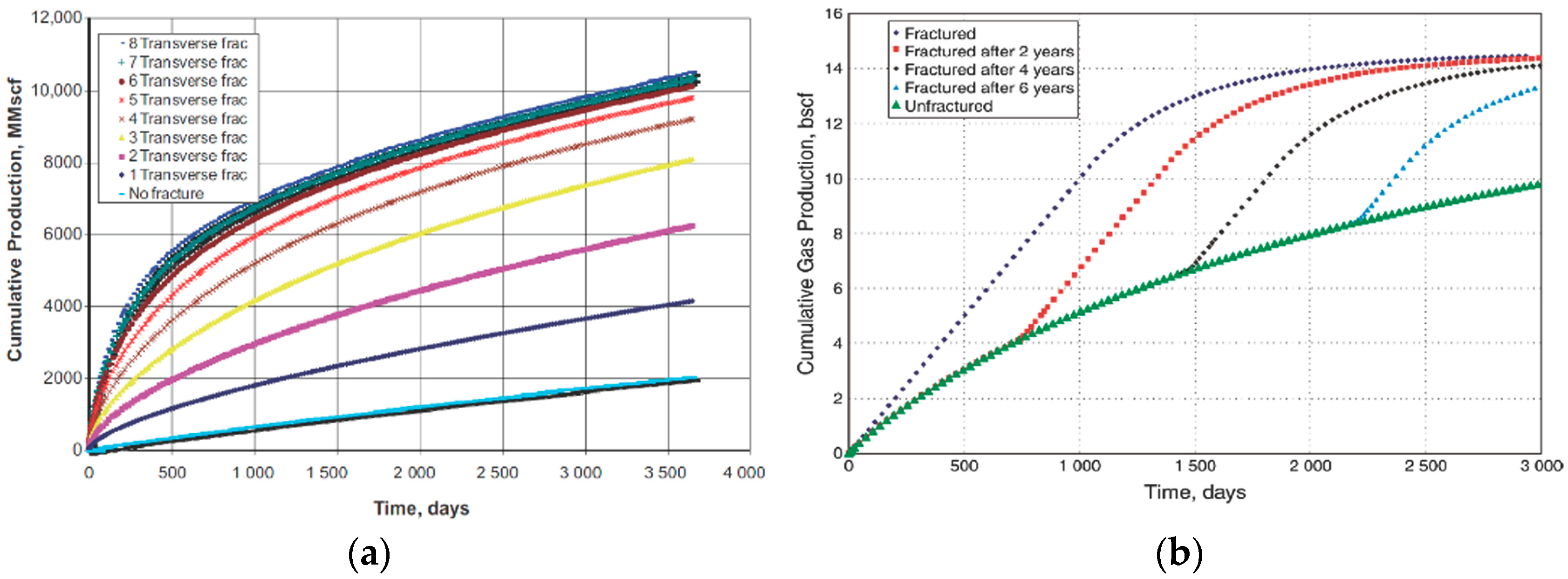
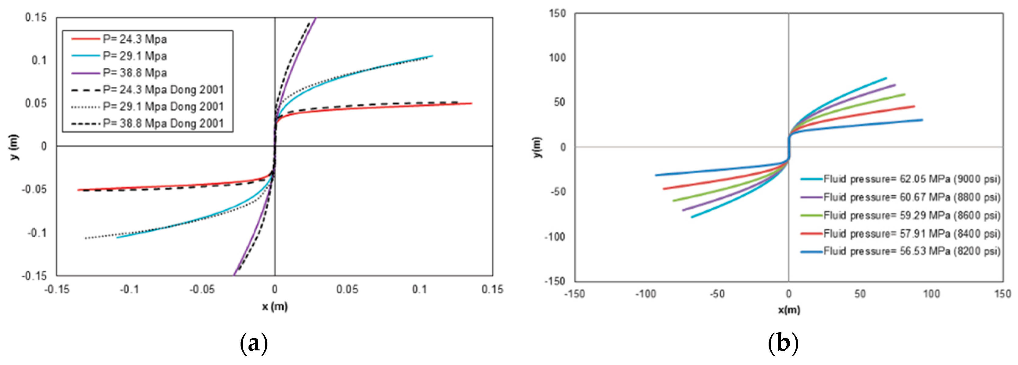
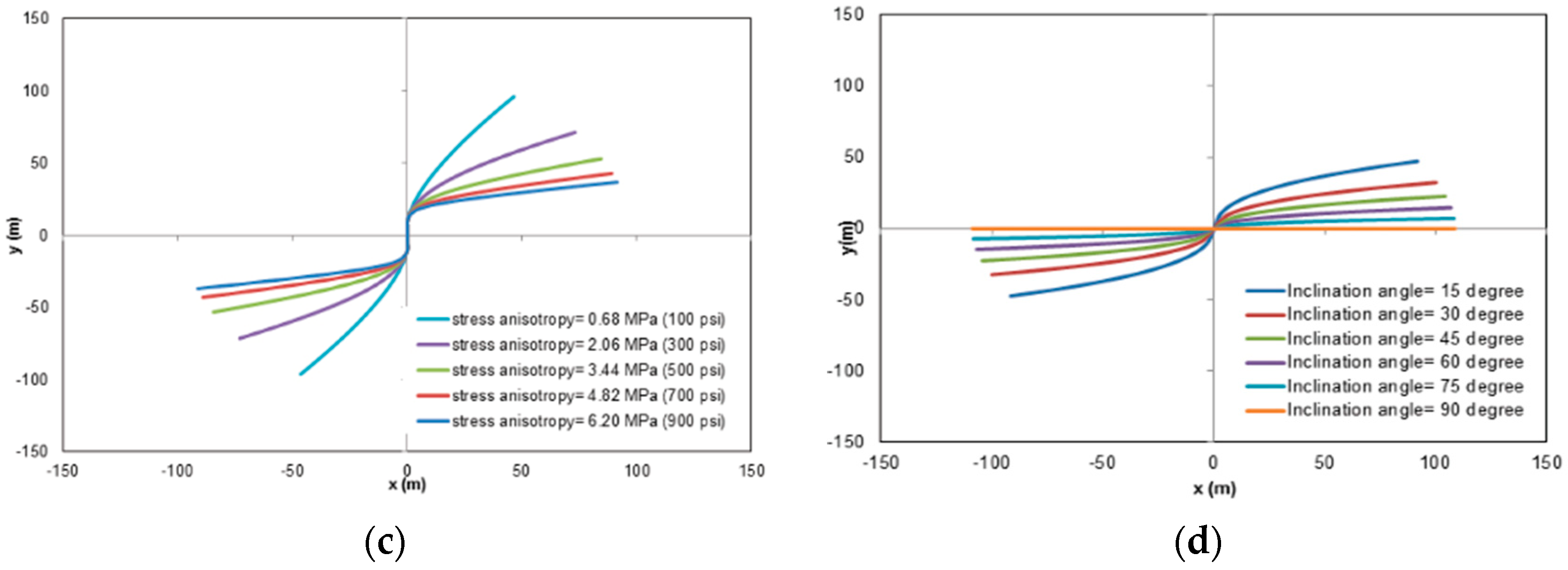
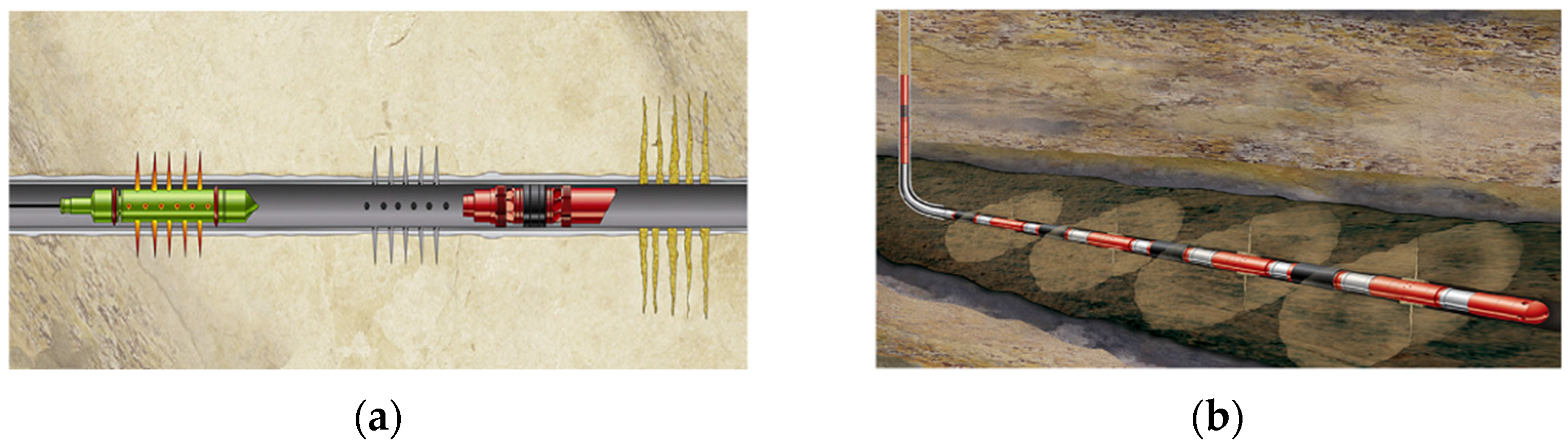


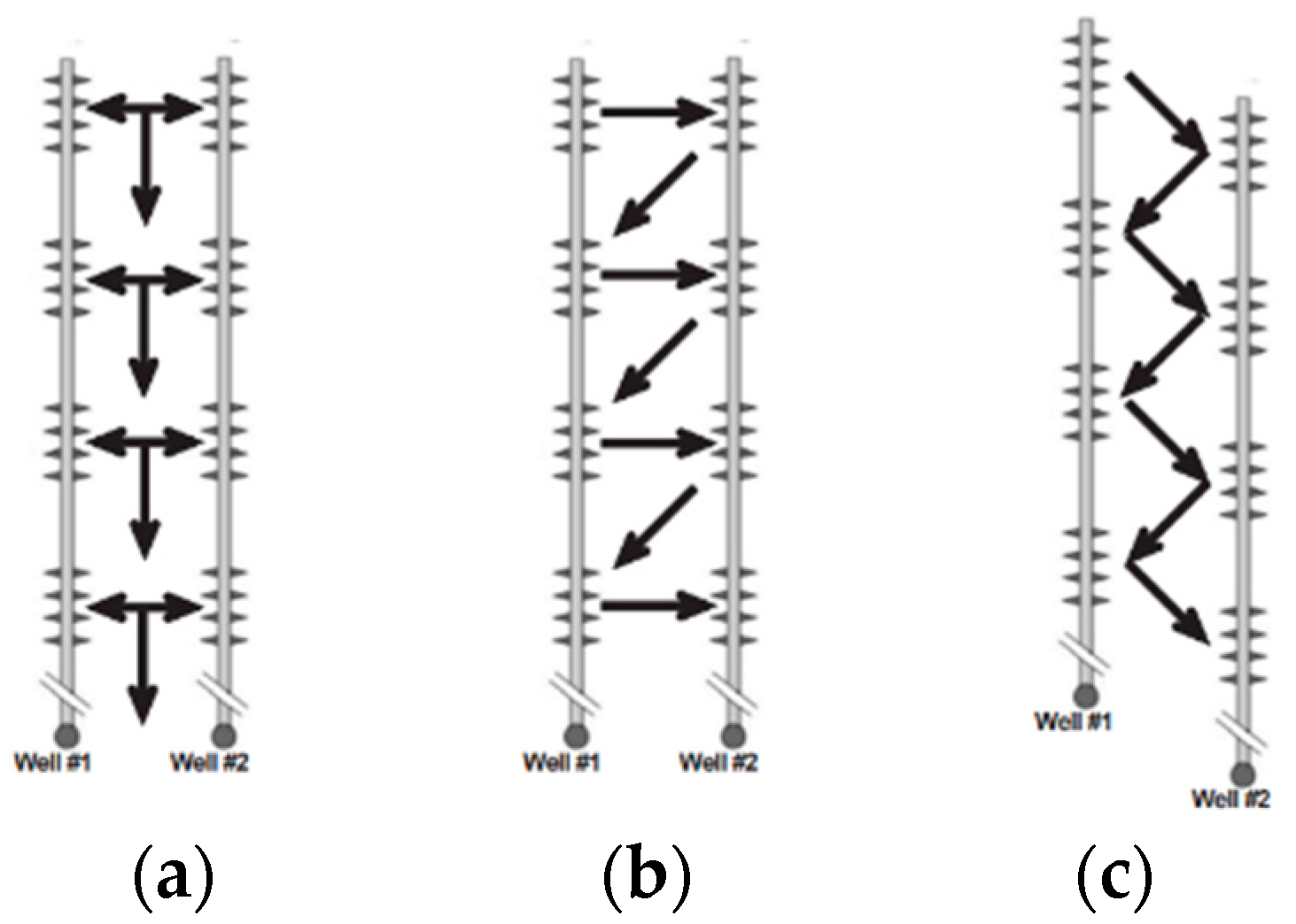
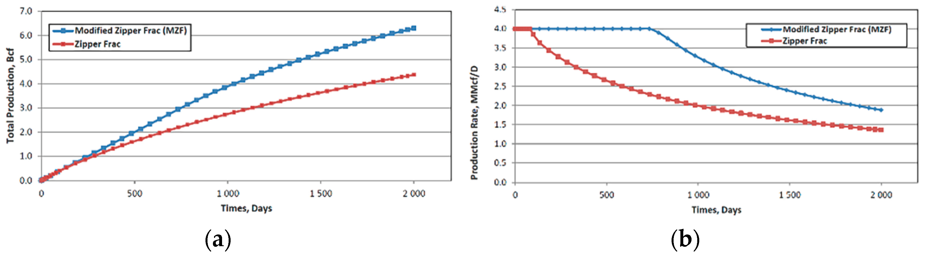
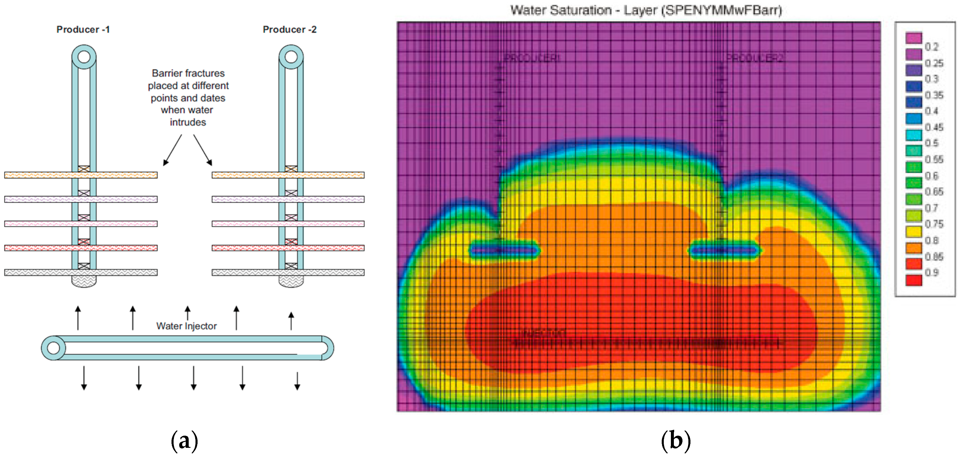
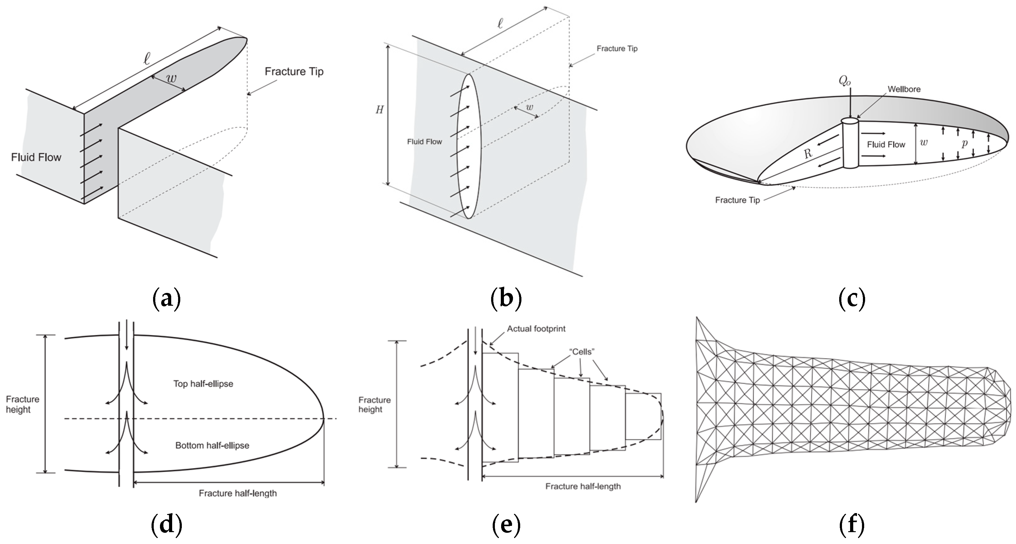
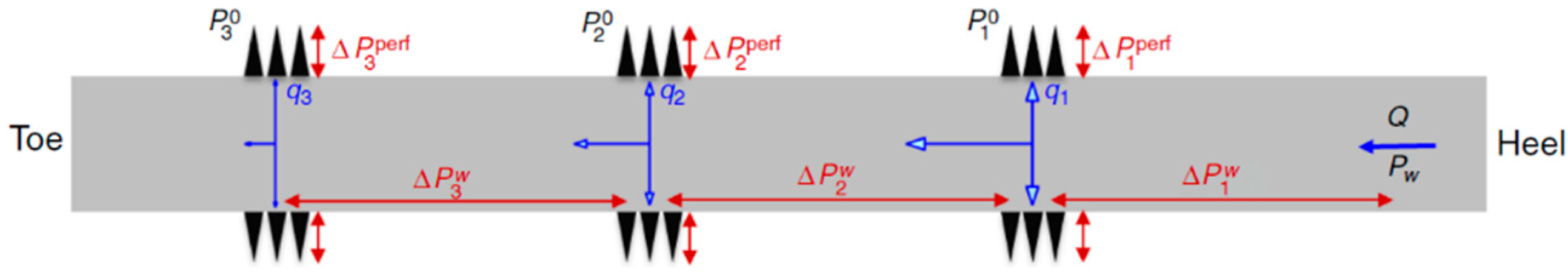


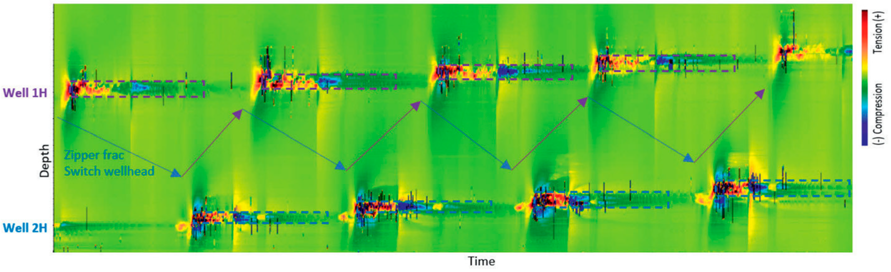
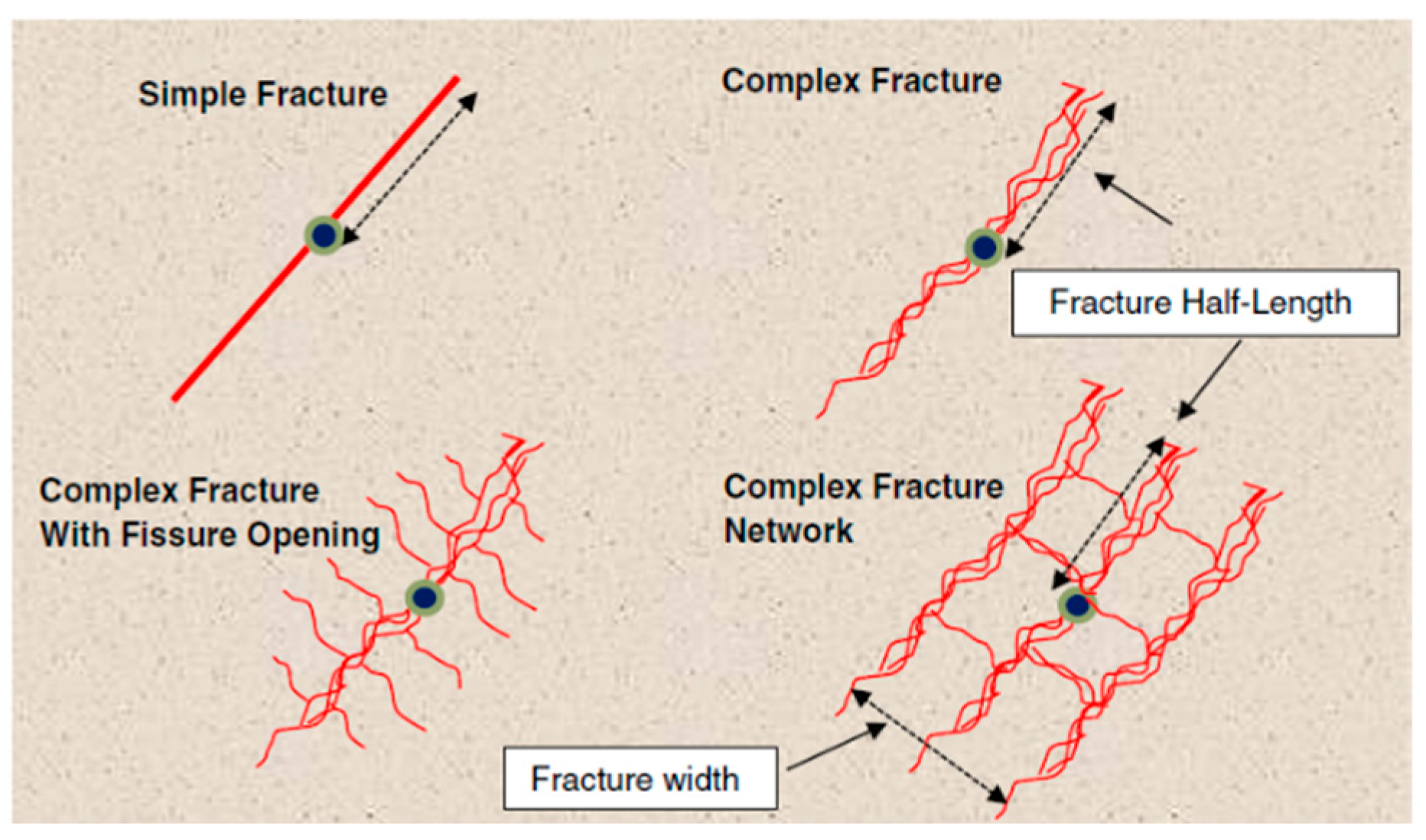
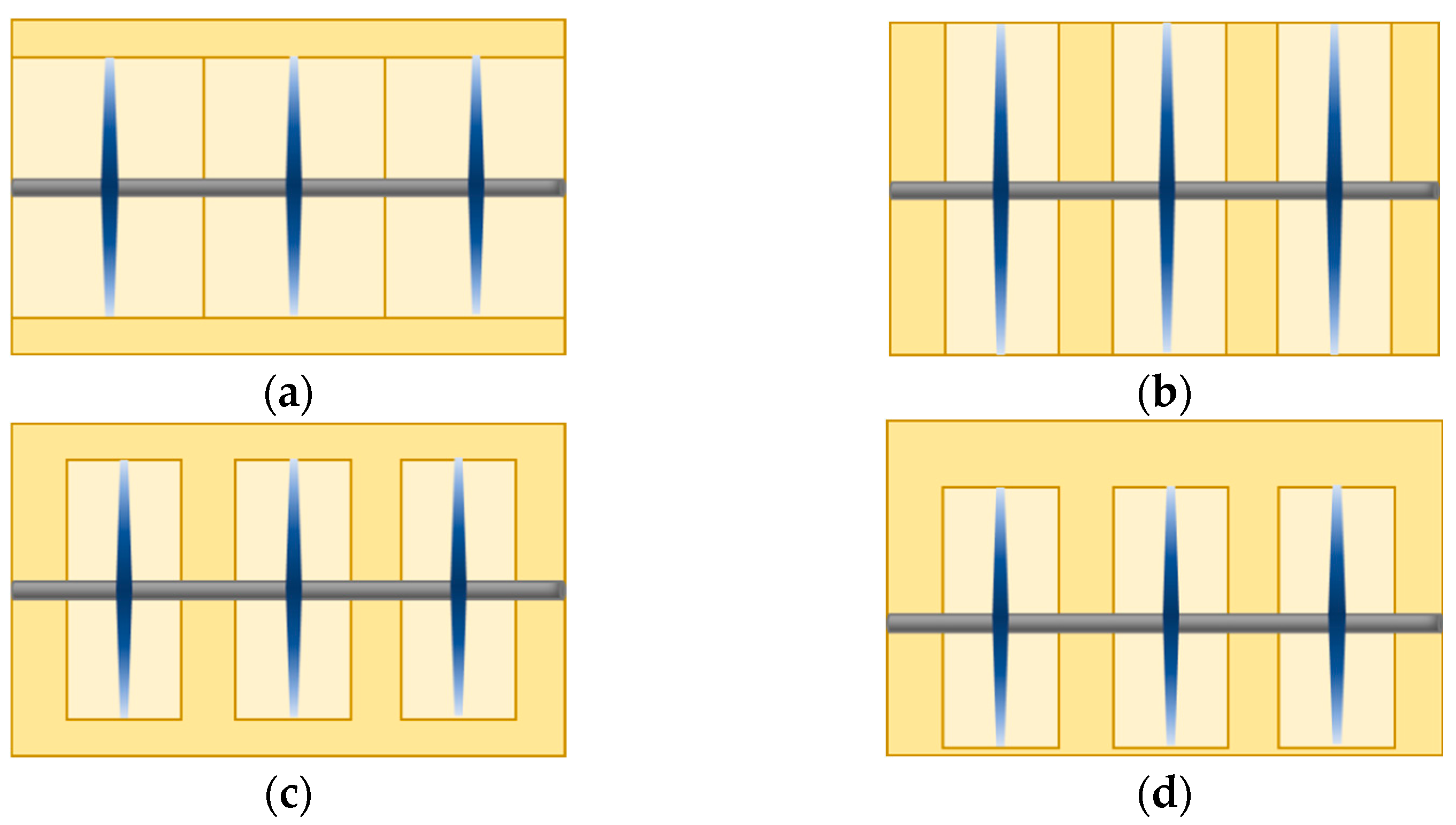
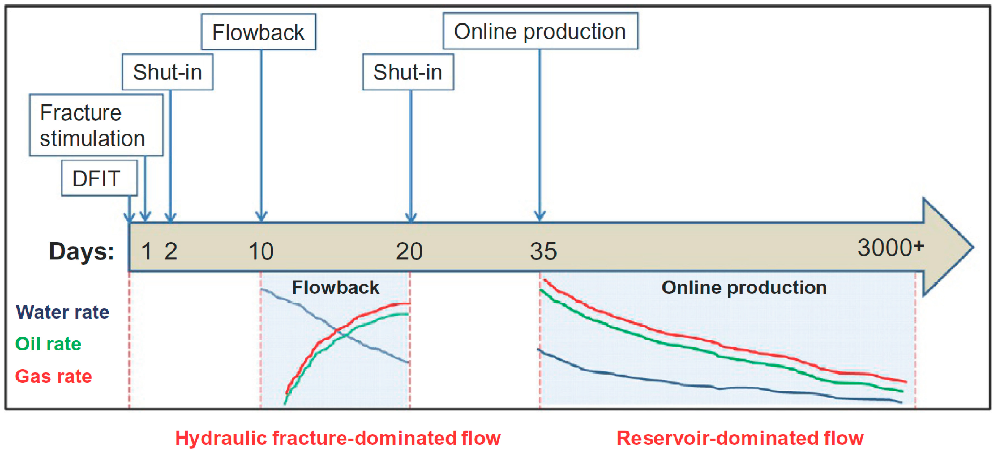
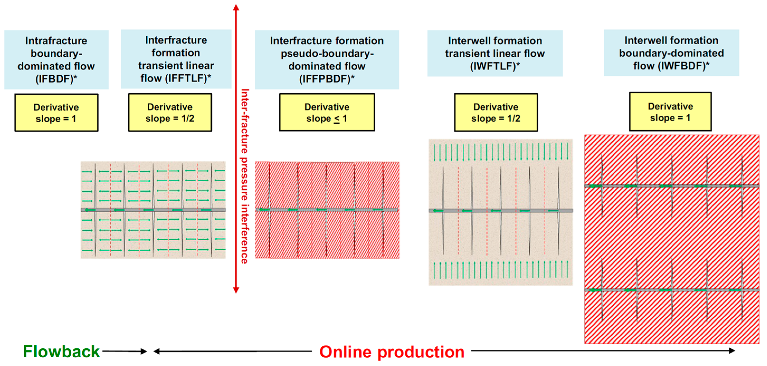
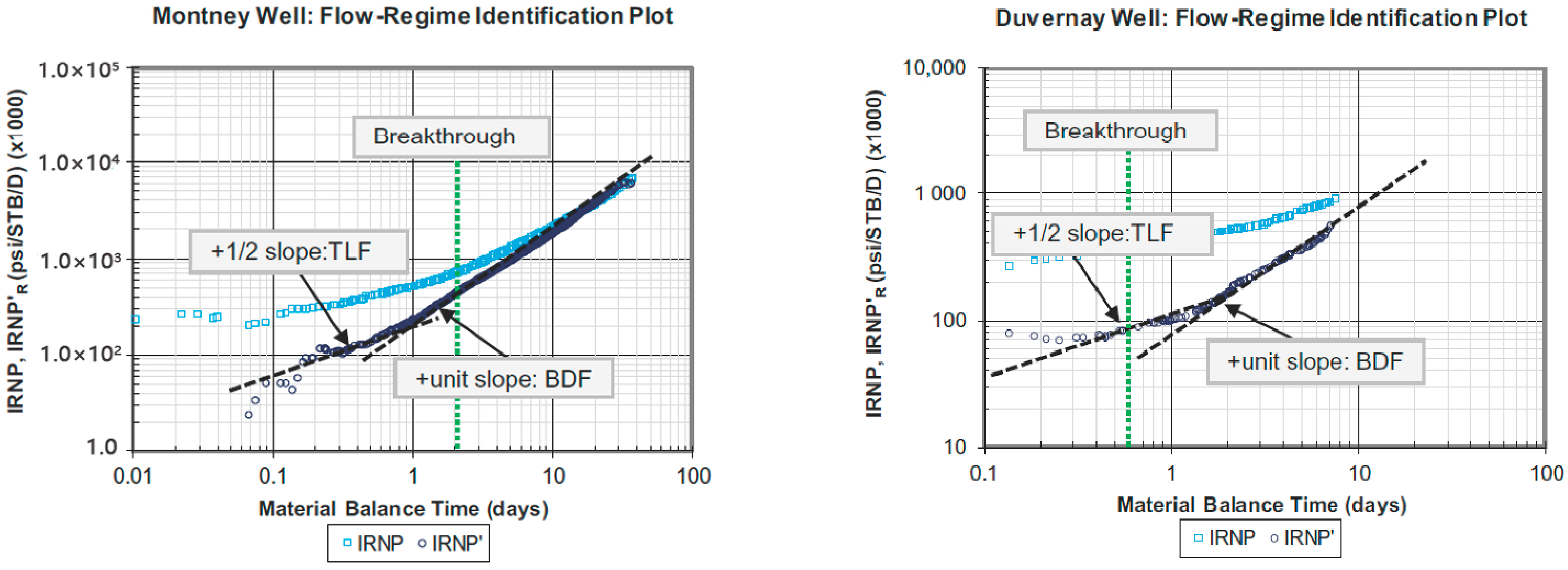
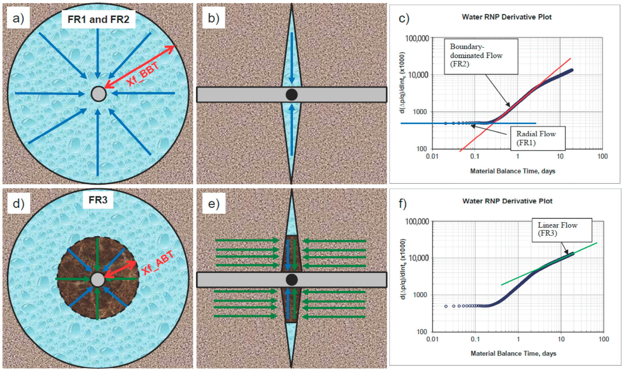
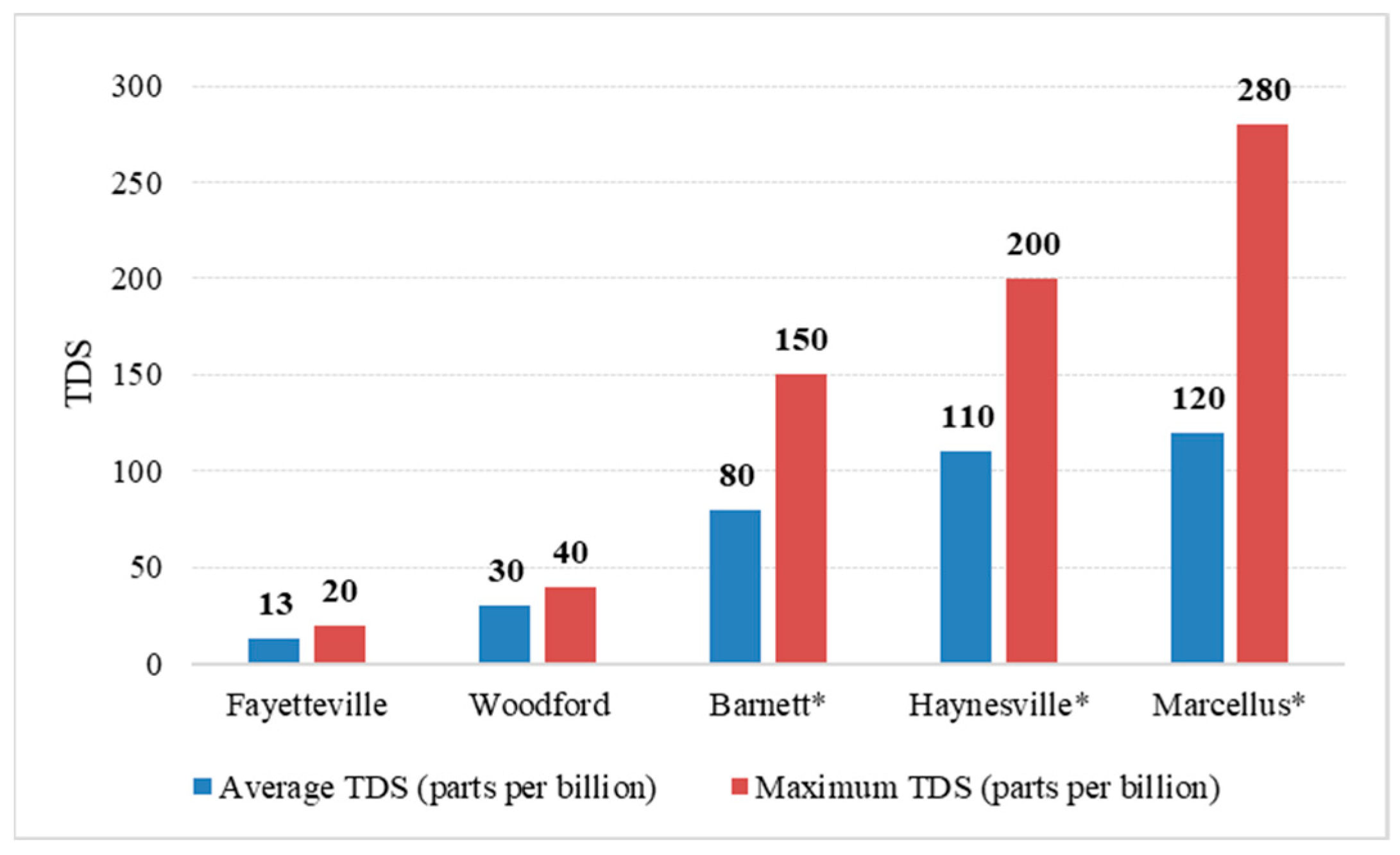

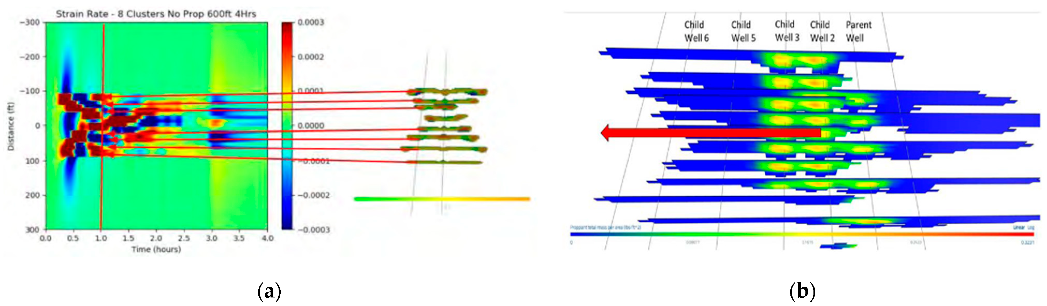
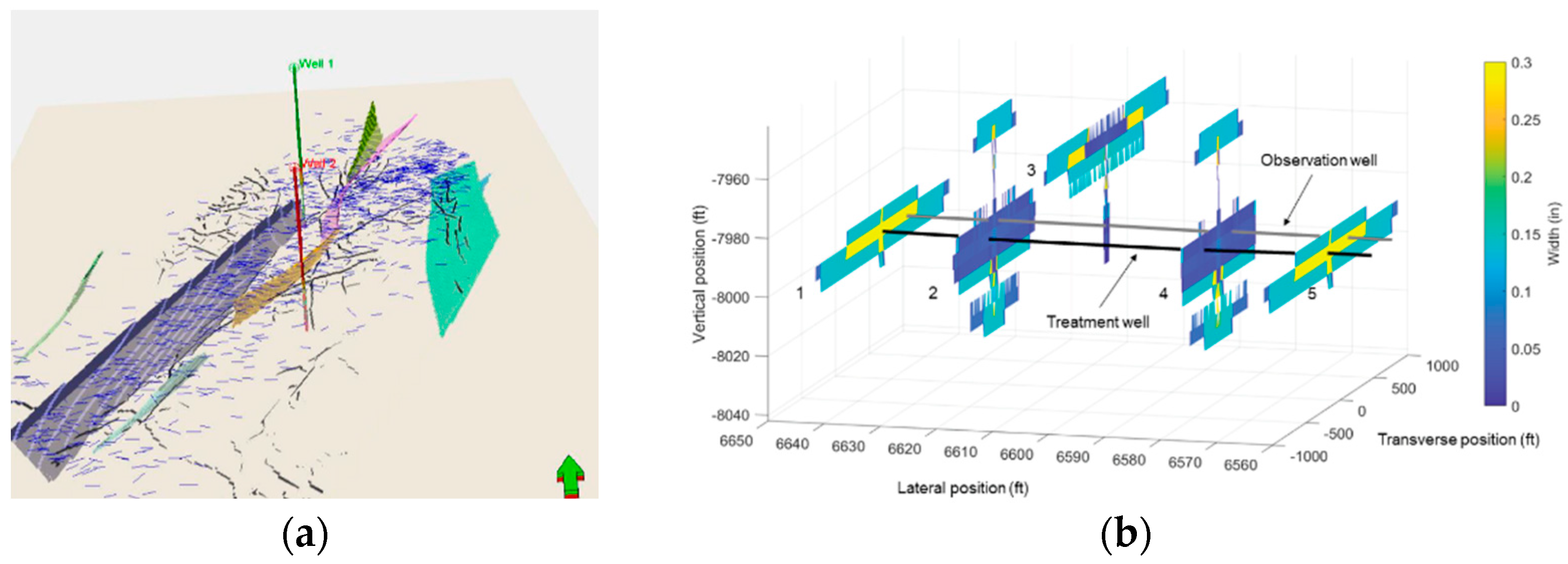

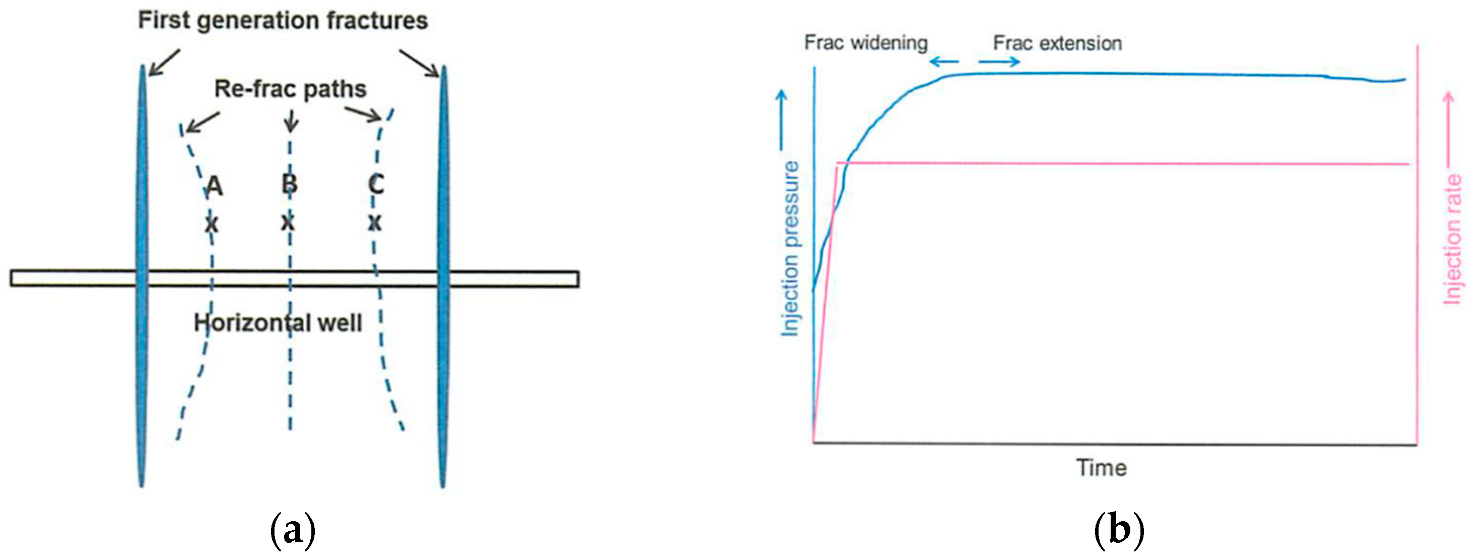
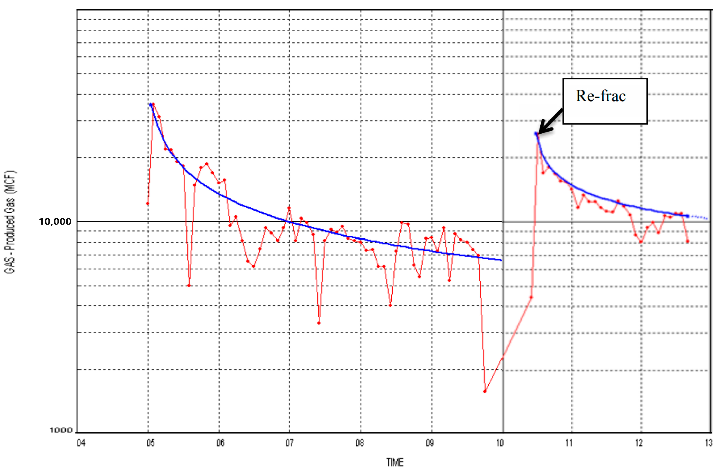
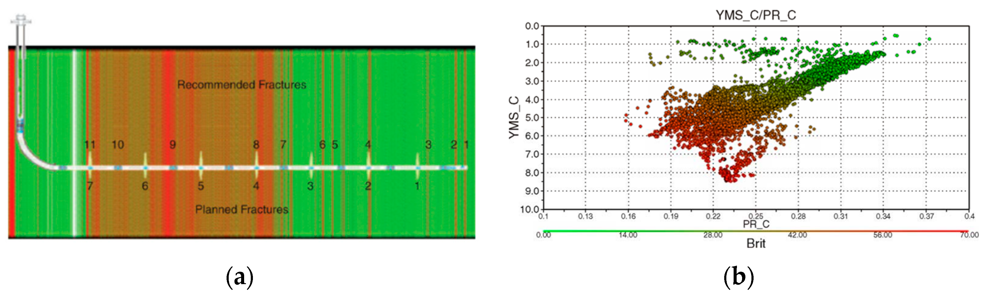

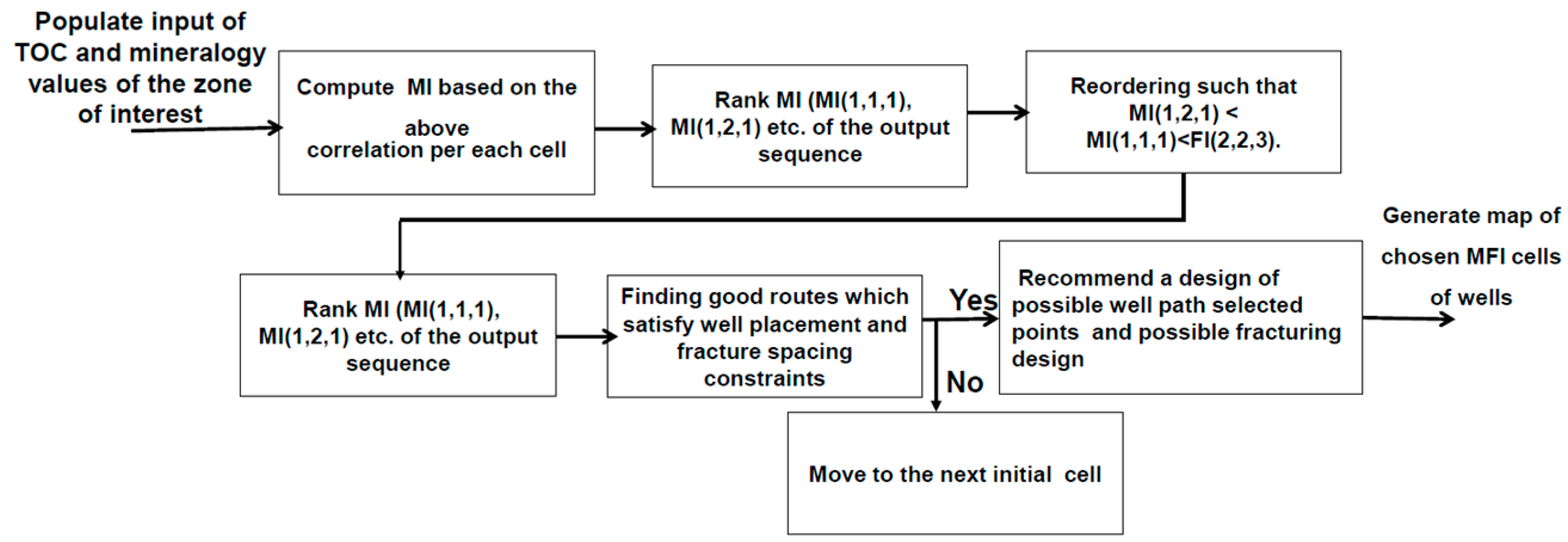
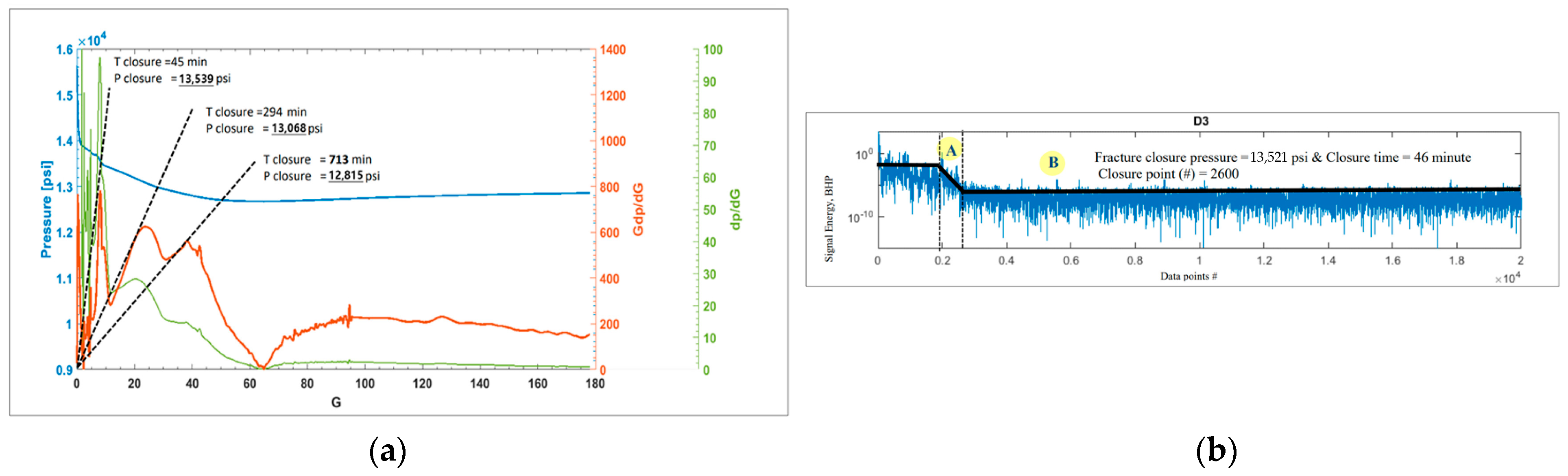
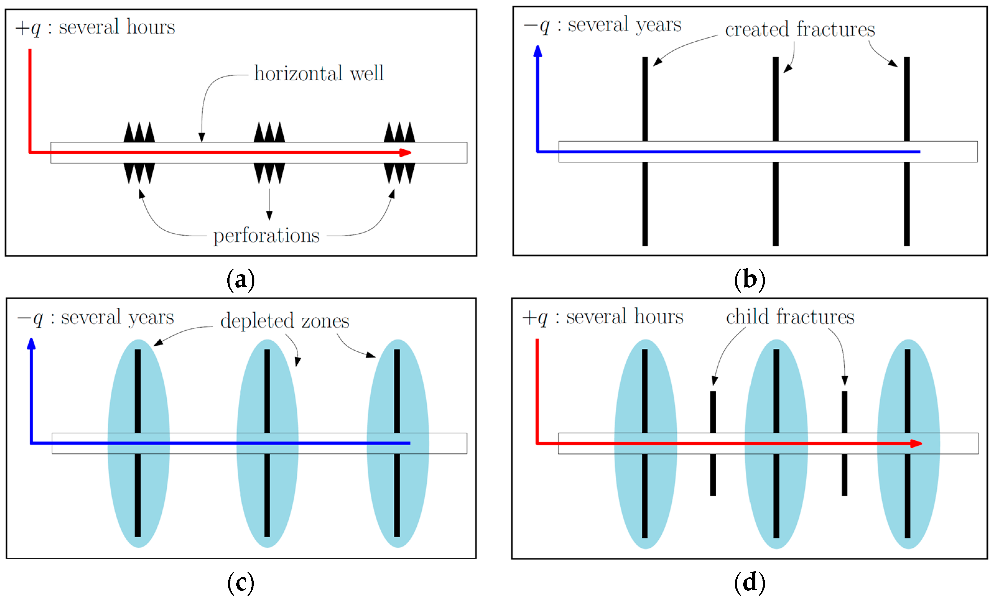
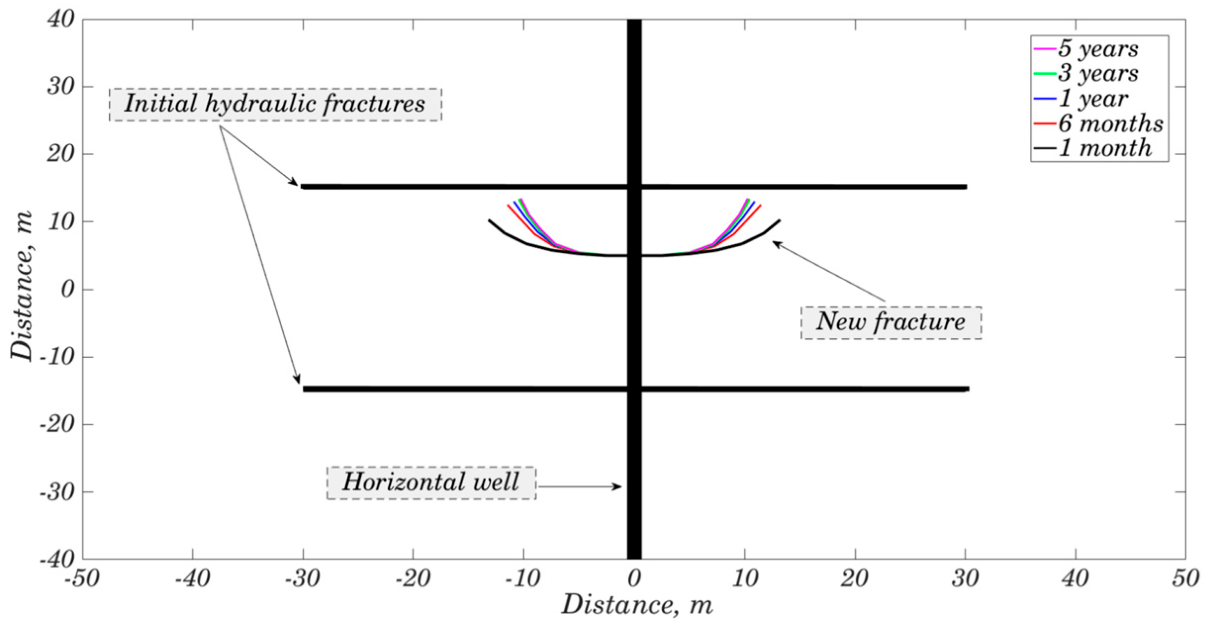

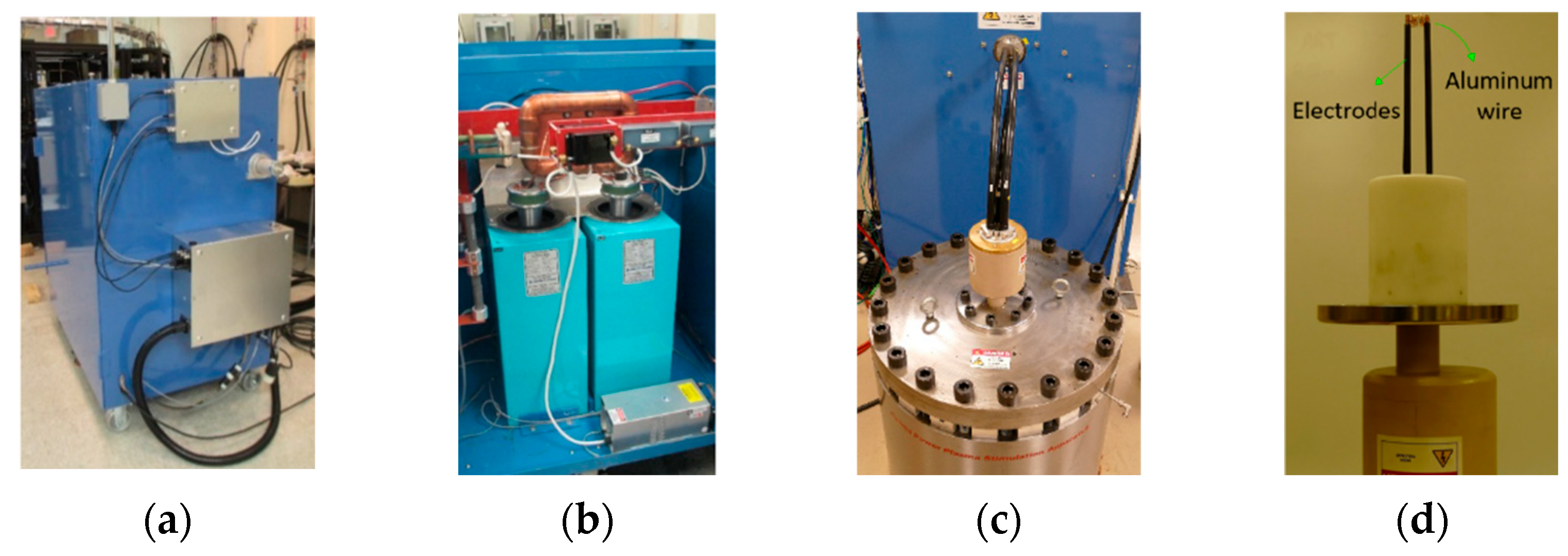

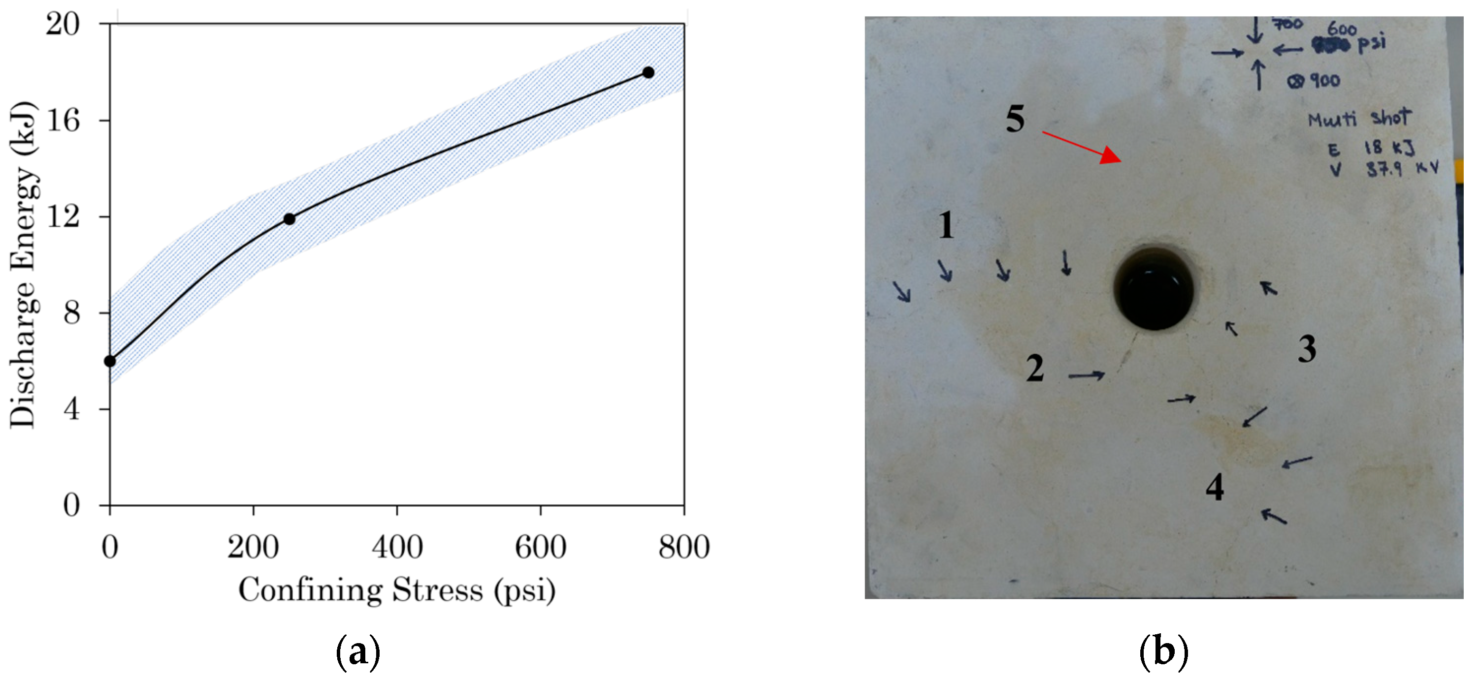

Disclaimer/Publisher’s Note: The statements, opinions and data contained in all publications are solely those of the individual author(s) and contributor(s) and not of MDPI and/or the editor(s). MDPI and/or the editor(s) disclaim responsibility for any injury to people or property resulting from any ideas, methods, instructions or products referred to in the content. |
© 2023 by the authors. Licensee MDPI, Basel, Switzerland. This article is an open access article distributed under the terms and conditions of the Creative Commons Attribution (CC BY) license (https://creativecommons.org/licenses/by/4.0/).