Condition Monitoring Method for the Gearboxes of Offshore Wind Turbines Based on Oil Temperature Prediction

Abstract

Traditional machine learning prediction methods usually only predict input parameters through a single model, so the problem of low prediction accuracy is common. Different predictive models extract different information for input, and combining different predictive models can make as much use as possible of all the information contained in the inputs. Therefore, this paper improves the existing oil temperature prediction method of offshore wind turbine gearboxes, and for the actual prediction effect of Supervisory Control And Data Acquisition (SCADA) data in this paper, Bayesian-optimized Light Gradient Boosting Machine (LightGBM) and eXtreme Gradient Boosting(XGBoost) machine learning models are selected to be combined. A method based on the Induced Ordered Weighted Average (IOWA) operator combination prediction model is thus proposed, with simulation results showing that the proposed model improves the accuracy of gearbox condition monitoring. The innovation of this article lies in considering the various negative impacts faced by actual offshore wind turbines and adopting a combination prediction model to improve the accuracy of gearbox condition monitoring.

1. Introduction

State monitoring technology refers to the monitoring of the real-time parameters of equipment during operation to determine whether there are any abnormalities in the equipment’s operating status. If the equipment is in an abnormal state, or has a tendency to transition to an abnormal state, an alarm signal is issued. Sometimes, for certain equipment or important components, condition monitoring technology can identify the fault location in the early stages of failure, buy sufficient time for maintenance personnel to work, and avoid unnecessary economic losses caused by equipment damage.

At present, there are two main methods for monitoring the status of offshore wind turbines and their gearboxes. One is the mechanistic modeling method, which involves physically modeling the entire wind turbine and its gearboxes and analyzing the source of faults; for example, Yang [1] conducted a thermal process analysis on the stator temperature of a permanent magnet synchronous motor in a wind farm. From a physical perspective, heat transfer knowledge was used to model the stator temperature and compare it with actual values to determine the state of the wind turbine; Sun [2] used oil spectrum monitoring technology to monitor the increment of iron elements in the gearbox oil of wind turbines and analyzed the operating status of the gearbox; and Zhang [3] used Lamb waves excited by parallel stress acting on wind turbine blades to locate the acoustic emission source of wind turbine blades, achieving state monitoring of wind turbine blades. Research based on mechanism modeling generally has clear physical significance and can effectively explain the mechanism of fault occurrence. However, wind turbines are a complex and massive system, and their modeling is based on a large amount of physical knowledge, such as sound, light, and heat due to differences in fault manifestations among various components, making it difficult to accurately express the physical models of the entire machine and gearbox. In recent years, thanks to the rapid development of SCADA technology, deep learning, and artificial intelligence, non-mechanistic modeling has gradually been widely used in the field of wind turbine faults. The use of deep learning models only requires the mining of information features contained in massive wind turbine SCADA data to establish normal behavior models for wind turbines and their key components [4]. For example, Jin [5] used a fusion sparse autoencoder to learn SCADA data under the normal operating conditions of wind turbines and predict wind power, achieving wind turbine status monitoring using the difference between predicted power and actual power. Liu [6] used a restrictive Boltzmann machine to establish a normal behavior model for wind turbines and used reconstruction errors to analyze the trend of changes in the operating status of wind turbines. Guo [7] adopted a fault early warning method of wind turbine pitch bearing based on SCADA data, input historical data, and the tags of state variables such as wind speed, pitch angle, and wind power into a random forest for training, subsequently predicting real-time data. Experiments show that this method can effectively improve the safe operation duration of the unit and reduce operation and maintenance costs. Therefore, this article intends to use non-mechanistic modeling methods to monitor the status of wind turbines and their gearboxes. Taking wind turbine gearboxes as the research object, deep learning models are used to fully learn the information contained in SCADA data during the normal operation of offshore wind turbines, thereby reducing the uncertainty of artificial design features and the dependence on subjective experience in mechanistic modeling.

The research methods for condition monitoring and fault diagnosis of wind turbine gearboxes include vibration signal analysis, oil temperature analysis, electrical signal-based analysis methods, and SCADA data analysis methods. At present, research on gearbox fault diagnosis is mainly based on gearbox oil temperature and vibration signals. Temperature signal monitoring is a commonly used method for monitoring gearbox faults in wind turbines. During the normal operation of wind turbines, the temperature changes of each component have a regular pattern to follow, so gearbox oil temperature is an indicator for the health of the gearbox [8].

There are two main methods for condition monitoring based on gearbox oil temperature. One is to model gearbox oil temperature through a thermal network. Xiang [9] studied the structure, control strategy, and thermodynamic behavior of wind turbine gearboxes, modeled the gearbox thermal network, calculated gearbox oil temperatures, and analyzed errors in relation to actual values. The simulation results show that the thermal network model can effectively detect faults in wind turbine gearboxes. Sun [10] conducted thermodynamic modeling analysis on the lubrication system of a wind turbine gearbox and obtained oil temperatures during stable operation of the wind turbine through the cyclic oil injection method. However, using thermodynamic modeling methods is not only time-consuming and labor-intensive, but also makes it difficult to obtain certain key parameters through direct measurement; thus, the limitations of its application are significant. The second method is to use data-driven state detection methods such as deep learning or machine learning. By collecting the real-time SCADA data of the gearbox and establishing the input and output connections of the wind turbine gearbox oil temperature prediction model, a highly accurate prediction value for wind turbine gearbox oil temperature can be obtained. Murgia [11] demonstrates the applicability of SCADA data to the fault diagnosis of wind turbines. Huang [12] used principal component analysis to reduce the dimensionality of wind turbine SCADA data and then used a dynamic neural network combined with statistical process control to model gearbox oil temperature. This method has high accuracy. Wan [13] used XGBoost to predict the temperature of the main bearings of wind turbines, obtained the residual values between the predicted values and the true values, and used the kernel density estimation method to obtain residual threshold values. Through the sliding window, the status of the main bearings of wind turbines was monitored. Experiments show that this method can predict faults in the main bearings of wind turbines in advance. With the development of data collection and monitoring systems, more and more scholars are using SCADA data as the research object of fault diagnosis technology. In response to the problem of limited and imbalanced oil temperature samples in gearbox time series, Li [14] improved the traditional deep convolutional generation adversarial network and proposed a Long Short-Term Memory Generative Adversarial Network (L-DCGAN) that can generate high-quality time series samples using the good adaptability of LSTM in processing time series. Experiments have shown that this model can track trends in signal time series changes, and the generated samples have time correlation. Wang [15] used Support Vector Machines (SVMs) and Back Propagation (BP) neural networks to predict the gear oil temperature of wind turbines, among which LS-SVM exhibited a good prediction effect. They proposed an LC-SVM gearbox oil temperature prediction method based on Kernel Principal Component Analysis (KPCA) and used statistical processes to monitor the status of wind turbine gearbox oil temperature. Experiments show that this method can detect faults early on and provide early warnings. From the above research, it can be seen that the main problem currently faced by using oil temperature for the condition monitoring of wind turbine gearboxes is that the prediction accuracy still needs to be further improved.

This paper takes the gearbox of offshore wind turbines as the research object and proposes a combined model based on an induced ordered weighted average operator. By predicting the oil temperature of the gearbox and mining the hidden feature information in the SCADA data of offshore wind turbines, it can accurately predict the operating status of the gearboxes of offshore wind turbines. Using SCADA real-time data from an offshore wind farm in Jiangsu Province for model effect simulation, an adaptive threshold condition monitoring method was used to predict the residual oil temperature of gearboxes. Experimental results show that the proposed algorithm exhibits a significant improvement in monitoring accuracy and can significantly reduce the probability of false alarms compared to traditional constant threshold monitoring methods.

2. Wind Turbine Condition Monitoring Algorithm Based on a Combined Prediction Model

Existing data-driven wind turbine condition monitoring algorithms often rely on machine learning or deep learning methods, though most use a single machine learning or deep learning model. In fact, the wind turbine is a complex nonlinear system, the components are coupled to each other, and it is difficult for a single model to mine the correlation between state variables and all the fault information implied in the input; thus, this paper proposes a Bayesian-based optimization of LightGBM and XGBoost. At present, some papers have demonstrated that the combination of the two models in load forecasting can achieve good results. Yao [16] used the Maximum Information Coefficient to filter the coat set of features and then used LightGBM and XGboost to filter key features that affect load forecasting, obtaining high-precision short-term load forecasting results. This represents a combined predictive model that leverages the information contained in the input state variables to achieve significant improvements in prediction accuracy compared to traditional single machine learning methods. In addition, an adaptive threshold method is used to monitor the residual condition of gearbox oil temperature prediction, which can effectively reduce the probability of false alarms in the model compared with the traditional constant threshold state monitoring method.

The wind turbine gearbox condition monitoring framework in this paper is shown in Figure 1. Firstly, the offline data are trained using the combined model based on Bayesian optimization of LightGBM and XGBoost, and the real-time data are then brought into the combined model based on the IOWA operator for prediction. The adaptive threshold is then used to monitor the residual oil temperature of the gearbox and issue an alarm when the threshold is exceeded.

2.1. XGBoost Principle

XGBoost is a kind of boosting machine learning algorithm that integrates different weak classifiers to form a strong learner, which has the characteristic of high precision and is not easy to overfit, thus leading to it being widely used in the field of data science. This paper uses XGBoost for oil temperature prediction of the gearboxes of offshore wind turbines. Compared with other machine learning methods, XGBoost comes with regularization terms, which can avoid model overfitting and lead to higher prediction accuracy. The objective function of XGBoost is shown in Formula (1):

$$Ob{j}^{\left(t\right)}={\displaystyle \sum _{i=1}^{n}l\left(y_i,{\widehat{y}}_i{}^{\left(t\right)}\right)+{\displaystyle \sum _{i=1}^t\Omega \left(f_i\right)}}$$

(1)

Here, $n$ indicates the number of samples and ${\widehat{y}}_i^{\left(t\right)}$ represents the predicate value for sample $i$ of the first $t$ trees. The first term on the right of the formula represents the loss value represented by the true value and the predicted value, and the second term on the right represents the regular term representing the sum of the complexity of the tree, which is to prevent the model from overfitting. The prediction results of the former $t$ tree on the model can be determined by the predicted outcome of the front $t-1$ trees and the predicted result of the $t^{th}$ tree. Formula is expressed as (2)

$${\widehat{y}}_i{}^{\left(t\right)}={\displaystyle \sum _{k=1}^t{f}_k\left(x_i\right)}={\widehat{y}}_i{}^{\left(t-1\right)}+f_t\left(x_i\right)$$

(2)

At this point, the objective function of the model can be written as shown in Formula (3):

$$\begin{array}{ll}Ob{j}^{\left(t\right)}& ={\displaystyle \sum _{i=1}^{n}l\left(y_i,{\widehat{y}}_i{}^{\left(t\right)}\right)+{\displaystyle \sum _{i=1}^t\Omega \left(f_i\right)}}\\ & ={\displaystyle \sum _{i=1}^{n}l\left(y_i,{\widehat{y}}_i{}^{\left(t-1\right)}+f_t\left(x_i\right)\right)}+{\displaystyle \sum _{i=1}^t\Omega \left(f_i\right)}\\ & ={\displaystyle \sum _{i=1}^{n}l\left(y_i,{\widehat{y}}_i{}^{\left(t-1\right)}+f_t\left(x_i\right)\right)}+\Omega \left(f_t\right)+constant\end{array}$$

(3)

The complexity of the first $t$ trees is split, and the regularization term of the objective function becomes the complexity of the tth tree plus the complexity of the first $t-1$ trees due to the complexity of the first $t$ trees being known; thus, the term is a constant. Making a Taylor expansion of the loss function in $y_i$ can be written as shown in Formula (4):

$$l\left(y_i,{\widehat{y}}_i{}^{\left(t\right)}\right)=l\left(y_i,{\widehat{y}}_i{}^{\left(t-1\right)}\right)+g_i{f}_t\left(x_i\right)+\frac{1}{2}{h}_i{f}_t^2\left(x_i\right)$$

(4)

where $g_i$ is the first derivative of the loss function, i.e., Formula (5). $h_i$ is the second derivative of the loss function, i.e., Formula (6):

$$g_i=\frac{\partial l\left(y_i,{\widehat{y}}_i^{\left(t-1\right)}\right)}{\partial {\widehat{y}}_i^{\left(t-1\right)}}=-2\left(y_i-{\widehat{y}}_i^{\left(t-1\right)}\right)$$

(5)

$$h_i=\frac{{\partial }^{2}l\left(y_i,{\widehat{y}}_i^{\left(t-1\right)}\right)}{\partial {\left({\widehat{y}}_i^{\left(t-1\right)}\right)}^2}=2$$

(6)

Bringing the loss function after Taylor expansion into the objective function yields Formula (7):

$$Ob{j}^{\left(t\right)}\simeq {\displaystyle \sum _{i=1}^n\left[l\left(y_i,{\widehat{y}}_i{}^{\left(t-1\right)}\right)+g_i{f}_t\left(x_i\right)+\frac{1}{2}{h}_i{f}_t^2\left(x_i\right)\right]}+\Omega \left(f_t\right)+constant$$

(7)

Removing the known values in the objective function has no effect on the optimization of the function, and the function that needs to be optimized is Formula (8):

$$Ob{j}^{\left(t\right)}\simeq {\displaystyle \sum _{i=1}^n\left[g_i{f}_t\left(x_i\right)+\frac{1}{2}{h}_i{f}_t^2\left(x_i\right)\right]}+\Omega \left(f_t\right)$$

(8)

The second item to the right of the formula, i.e., $\Omega \left(f_t\right)$, represents the complexity of the first $t$ trees and is determined by the leaf node tree of the tree; the more leaf nodes and the more complex the tree, the higher the model accuracy, though too many leaf nodes lead to model overfitting more often. This subsequently leads to the dataset manifesting high accuracy with the training set but low accuracy with the test set. The complexity of tree $t$ can be expressed as shown in Formula (9):

$$\Omega \left(f_t\right)=\gamma T+\frac{1}{2}\lambda {\displaystyle \sum _{j=1}^T{\omega }_j^2}$$

(9)

where $T$ indicates the number of leaves in the tree and ${\omega }_j^2$ represents the weight vector of leaf nodes in a Norm $L_2$. Bringing complexity as an objective function regular term into the equation yields Formula (10):

$$\begin{array}{ll}Ob{j}^{\left(t\right)}=& {\displaystyle \sum _{i=1}^n\left[g_i{f}_t\left(x_i\right)+\frac{1}{2}{h}_i{f}_t^2\left(x_i\right)\right]}+\Omega \left(f_t\right)\\ & ={\displaystyle \sum _{i=1}^n\left[g_i{f}_t\left(x_i\right)+\frac{1}{2}{h}_i{f}_t^2\left(x_i\right)\right]}+\gamma T+\frac{1}{2}\lambda {\displaystyle \sum _{j=1}^T{\omega }_j^2}\end{array}$$

(10)

Bringing the sample into the $t^{th}$ tree to obtain the relationship with the leaf nodes results in Formula (11):

$$f_t\left(x\right)={\omega }_{t\left(x\right)},\omega \in R^T,t:R^d\to \left\{1,2,\cdots ,T\right\}$$

(11)

where $\omega$ represents the weight corresponding to each leaf node in tree $t$ and $t$ represents the structure of the tree with $T$ leaf nodes. The objective function is finally sorted out into Formula (12):

$$\begin{array}{ll}Ob{j}^{\left(t\right)}& ={\displaystyle \sum _{i=1}^n\left[g_i{f}_t\left(x_i\right)+\frac{1}{2}{h}_i{f}_t^2\left(x_i\right)\right]}+\gamma T+\frac{1}{2}\lambda {\displaystyle \sum _{j=1}^T{\omega }_j^2}\\ & ={\displaystyle \sum _{i=1}^n\left[g_i{\omega }_t\left(x_i\right)+\frac{1}{2}{h}_i{\omega }_t^2\left(x_i\right)\right]}+\gamma T+\frac{1}{2}\lambda {\displaystyle \sum _{j=1}^T{\omega }_j^2}\\ & ={\displaystyle \sum _{i=1}^n\left[\left({\displaystyle \sum _{i\in I_j}{g}_i}\right){\omega }_j+\frac{1}{2}\left({\displaystyle \sum _{i\in I_j}{h}_i+\lambda }\right){\omega }_j^2\right]}+\gamma T\end{array}$$

(12)

where $I_j$ indicates the collection of training samples in the $j^{th}$ leaf node.

2.2. LightGBM Algorithm

Due to the huge amount of SCADA data from offshore wind turbines, the application of traditional boosting algorithms such as gradient boosting trees and XGBoost is computationally intensive, making it difficult to balance accuracy and efficiency. The Light Gradient Boosting Machine (LightGBM) algorithm does not need to scan all sample points, meaning training is more efficient, takes less time, and does not take up a lot of memory. Therefore, this paper considers the LightGBM algorithm for research. The LightGBM algorithm is a high-performance machine learning tool that the Microsoft DMTK team open-sourced on GitHub and was improved from the framework of the XGBoost algorithm, mainly through the following improvements:

(1) Construction of a decision tree algorithm based on a histogram algorithm: The continuous floating-point features are constructed into a bin with width K, and then the training data are traversed to count the amount of data in each discrete histogram. When training, it is only necessary to traverse the discrete value of the bin to find the optimal segmentation point. A leaf node in the LightGBM algorithm can be obtained by the difference between the parent node and the sibling node, and when constructing the histogram, only K. bins of the histogram need to be traversed. The advantage of this improvement is that the originally huge data occupy less memory during calculation, reducing the complexity and calculation time of the data. Figure 2 shows a schematic diagram of the histogram algorithm.

(2) Maximize growth strategy according to leaf information gain: The growth strategy of traditional gradient boosting trees is to split and grow each leaf node in a layer at the same time, as shown in Figure 3. This is not computationally efficient and prone to overfitting. LightGBM, on the other hand, uses a per-leaf growth strategy with depth restrictions, as shown in Figure 4, where only the leaf nodes with the largest gain are split each time they grow.

(3) Unilateral gradient sampling method: Since samples with smaller gradients contribute less to information gain, it is necessary to exclude most of the samples with small gradients under the premise of ensuring accuracy, thus only using the remaining samples to calculate information gain. This algorithm needs to weigh the amount of data in the sample and the accuracy of the calculation result, and compared with random sampling under the same amount of data, the algorithm can obtain a more accurate effect when the information gain range is large.

(4) Exclusive Feature Bundling (EFB): In practical applications, data at high latitudes are often sparse, and many features rarely take non-zero values at the same time, that is, mutually exclusive features. The algorithm binds multiple mutually exclusive features together so they become dense features at low latitudes, which can effectively avoid unnecessary calculation of 0-feature values.

Compared with the traditional boosting algorithm, the LightGBM algorithm mainly consists of the following advantages:

(1) The LightGBM algorithm does not need to traverse all the data, only the discrete data in the sample histogram, which greatly reduces the calculation time;

(2) The histogram algorithm uses bin instead of the original discrete data, that is, some details of the data are lost during training, so the LightGBM algorithm can reduce the risk of overfitting to a certain extent;

(3) During the training process, the LightGBM model only retains samples with large gradients under the premise of ensuring certain calculation accuracy, which greatly reduces the amount of calculation;

(4) The LightGBM model adopts a leaf-wise decision tree growth strategy, which reduces the amount of computation and reduces the risk of overfitting;

(5) In the training process, the LightGBM model adopts a mutually exclusive feature bundling algorithm to reduce the number of features and reduce the memory footprint.

2.3. Bayesian Hyperparameter Optimization

Since the LightGBM model contains many training hyperparameters that need to be entered manually, such as learning rate, number of iterations, tree depth, number of leaves, feature sampling, etc., and because different parameter input combination methods have a certain degree of influence on the model results, it is necessary to use the parameter tuning tool in the model to find the best parameters possible.

Traditional parameter tools include grid search, random grid search, etc. Grid searching is performed to verify all points as much as possible in a parameter space, so it often consumes a lot of computing resources. Random searching finds the approximate optimal solution through random sampling in the search range, which improves search efficiency; however, the results obtained are quite different from each other, and it is easy to fall into the local optimal solution. Bayesian optimization is a state-of-the-art hyperparameter optimization tool in the field of black-box function estimation. Compared with traditional parameter adjustment tools, Bayesian optimization adopts a Gaussian process, which fully considers the parameter information of the previous step during calculation and has the advantages of fast calculation speed, a lower number of iterations, and robustness toward non-convex problems.

The Bayesian optimization parameter problem can be defined as a problem in which the function input is unknown and the maximum value is evaluated, i.e., Formula (13):

$$\stackrel{\ast }{x}=\underset{x\in X}{\arg \min }f\left(x\right)$$

(13)

where $x$ represents the hyperparameters of the model; $f\left(x\right)$ represents the objective function, which in this paper is the loss function of the model; and $X$ represents the search space for hyperparameters. The purpose of parameter tuning is to find the global best advantage that makes the loss function value the smallest while finding the global optimum hyperparameter. The traditional gradient descent algorithm is used to gradually achieve the maximum value through the derivative of the function, but when the objective function is too complex or unknown, the derivation becomes extremely difficult and requires a lot of computing resources. Bayesian optimization regards the objective function as a sampling of the Gaussian process distribution a priori and measures the best advantages of the approximation function by repeatedly measuring the objective function, and its core is to determine the next parameter to be tried based on existing observations.

The Bayesian optimization process can be summarized in four steps:

(1) Define the objective function f(x) and the hyperparameter search space X;

(2) Randomly take n observation points and find the observation values;

(3) Estimate the function based on these n observations;

(4) Determine the next observation point according to the collection function, thus forming a new observation history and resulting a return to step (3) until the computing resources are exhausted.

2.4. Combinatorial Prediction Model Based on the IOWA Operator

In the field of prediction, how to improve the accuracy of models has always been the focus of scholars’ research. The accuracy of traditional single machine learning prediction algorithms is often unsatisfactory, and in order to further optimize model accuracy, Yager [17] introduced IOWA to establish an information fusion model, which is widely used in the field of load forecasting. Chu [18] studied LSTM, XGBoost, GBDT, SVM, and other load forecasting models and found that the combined model is superior to the single model in terms of accuracy. Therefore, this paper will use a combinatorial prediction method based on the IOWA operator [19] to optimize LightGBM and XGBoost for Bayesian operations. The model takes the weights and obtains the combined prediction results. The principle of the IOWA operator combination model is as follows:

Suppose there are $n$ single predictive models, represented as $n$ two-dimensional arrays $\left(\langle v_1,a_1\rangle ,\langle v_2,a_2\rangle ,\cdots ,\langle v_n,a_n\rangle \right)$. The expression of the induced ordered weighted average operator is then composed of $n$ single models, as shown in Formula (14):

$$IOW{A}_W\left(\langle y_1,v_1\rangle ,\langle y_2,v_2\rangle ,\cdots ,\langle y_n,v_n\rangle \right)={\displaystyle \sum _{i=1}^n{w}_i{y}_{v-index\left(i\right)}}$$

(14)

where $v_i$ represents the inducing value of $y_i$, $v-index\left(i\right)$ represents subscript corresponding to the number $v_1,v_2,v_3,\cdots ,v_n$ in order from largest to smallest, the ordered weight vector for each single model is $W=\left(w_1,w_2,\cdots ,w_n\right),{\displaystyle \sum _{i=1}^n{w}_i=1}$, and $w_i$ is the weights of model $i$. It can be seen from this formula that the IOWA operator is the weighted sum of the predicted values of each single model after sorting the induced values from largest to smallest. $w_i$ is not related to the location of the accuracy of each individual model, but instead refers to the location of the model-induced value. The formula for prediction accuracy of a single model in moment $t$ is Formula (15):

$$A_{it}=\{\begin{array}{cc}1-\left|\frac{y_t-y_{it}}{y_t}\right|& ,\frac{y_t-y_{it}}{y_t}<1\\ 0& ,\frac{y_t-y_{it}}{y_t}\ge 1\end{array}$$

(15)

where $y_t$ represents the actual value at moment $t$ and $y_{it}$ representative the predicted value of model $i$ at moment $t$. This article puts the prediction accuracy $A_{it}$ as an induced value of model $i$ at moment $t$ and sorts the model prediction value from largest to smallest in terms of accuracy. The predicted values at moment $t$ of the combined model are shown in Formula (16):

$${\widehat{y}}_t={\displaystyle \sum _{i=1}^n{w}_i{y}_{v-index\left(it\right)}}$$

(16)

where ${\widehat{y}}_t$ represents the combination model prediction value at moment $t$ and $y_{v-index\left(it\right)}$ is the ith model ranked in order of induced value from largest to smallest models. The weights are selected using the criterion of minimizing the sum of squared prediction errors in the combined model, and the optimization objective function is expressed in Formula (17):

$$\begin{array}{l}\min S\left(W\right)={{\displaystyle \sum _{t=1}^T\left(y_t-{\displaystyle \sum _{i=1}^n{w}_i{y}_{a-index\left(it\right)}}\right)}}^2\\ s.t.{\displaystyle \sum _{i=1}^n{w}_i=1}\end{array}$$

(17)

The ordered weight $W$ vectors of each combined model can be obtained by solving the above objective function optimal value by using the nonlinear specification with constraints. In this paper, the conjugate gradient method is used to solve the optimal value of the weight vector.

2.5. Adaptive Thresholds

Since the operation of wind turbines has non-stationary characteristics, the residual between the predicted value of gearbox oil temperature and the true value is also in a state of dynamic change, and due to the influence of environmental noise, the residual value fluctuates greatly; thus, the residual processing method is first smoothed by exponential smoothing [20]. The smoothed residual value at the current time is equal to the weighted sum of the residual value at the previous time and the residual value at the current time, as shown in Formula (18):

$$R_t{}^{\prime }=\alpha R_t+\left(1-\alpha \right)R_{t-1}{}^{\prime }$$

(18)

where ${R^{\prime }}_t$ indicates the smoothed value of the residual at moment $t$. $\alpha$ represents the smoothing factor.

It can be seen that the residual after smoothing and the residual at the current moment are related to the residual smoothing value of the previous moment. If the alarm line is set with a constant threshold, the standard deviation of the residuals may become very small due to smoothing, in which case a constant threshold method is used. When the $3\sigma$ threshold is set, the threshold may be very close to the mean residual value, and if the operating conditions of the wind turbine change slightly, it easily causes false alarms.

Therefore, this paper calculates the standard deviation of the initial residuals so that the alarm threshold changes with time, thereby reducing the probability of false alarms [21]. Considering that the actual offshore wind turbine is in a noisy operating environment, this paper measures noise using the average rate of change in the residuals and weakens its influence on condition monitoring. The exact expression is Formula (19):

$$\dot{Y}=\frac{{\displaystyle \sum _{t=1}^{k-1}\left(y_{t+1}-y_t\right)}}{k-1}$$

(19)

where $k$ represents sample length and $\dot{Y}$ is the average rate of change in noise over that period. We then consider the noise factor in the adaptive threshold, as expressed in Equation (20):

$$U\left(t\right)=R_t{}^{\prime }\pm \left(\dot{Y}+\sigma \right)$$

(20)

where $U\left(t\right)$ represents the alarm threshold at moment $t$, with the value of $n$ taken as 3 from Ref. [21].

When the offshore wind turbine gearbox is in an abnormal state, the distribution characteristics of oil temperature are destroyed, which is manifested by a sudden increase in the difference between the true value and the predicted value, at which time the residual falls outside the alarm threshold range and an alarm is issued. Considering the changes in the operating conditions of the wind turbine, if a constant alarm threshold is used it is likely that the normal residual is beyond the warning range due to the change in residual distribution characteristics. Therefore, using adaptive thresholds to monitor residual changes can find faults more accurately. The abnormal determination criterion of the gearboxes of wind turbines is shown in Formula (21):

$$\{\begin{array}{c}{R}_t>U\left(t\right),\mathrm{Alarm}\\ R_t<U\left(t\right),\mathrm{Normal}\end{array}$$

(21)

3. Example Analysis

Real-time SCADA data describing the oil temperature of the gearbox of the No. 01 wind turbine of an offshore wind farm in Jiangsu in the first half of 2021 were selected as the experimental object, and the dataset was divided into a training set and a test set. Considering the harsh environment of the actual offshore wind turbine, the SCADA dataset contains a large number of outliers, missing values, and other abnormal data, so it is necessary to preprocess the SCADA data before using the machine learning method for prediction. First, a box plot is used to quickly identify the data distribution characteristics of each state variable and delete the abnormal data points. Then, for the missing data, the random forest interpolation method is used to complete the time series data. Finally, all parameters are normalized. The test set is brought into the trained model, the residuals of the predicted and true values are found, and the residuals are then brought into the LightGBM network based on Bayesian optimization. The SCADA data status variables are shown in

Table 1. SCADA data status variables.

Number	Variable
V1	Generator rear bearing temperature
V2	The amount of bearing temperature in front of the generator
V3	30 s average wind speed
V4	Wind cabin temperature
V5	Temperature outside the cabin of the wind turbine
V6	Gearbox high-speed shaft generator side bearing 1 temperature
V7	Gearbox high-speed shaft generator side bearing 2 temperature
V8	Gearbox oil temperature
V9	Generator stator U temperature
V10	Generator stator V temperature
V11	Generator stator W temperature
V12	Hub temperature
V13	Tower temperature
V14	Gearbox bearing vibration value
V15	Cabin X-axis vibration value
V16	Cabin Y-axis vibration value
V17	Annual availability of wind turbines
V18	Daily power generation of wind turbines
V19	10 min average wind speed

.

3.1. Data Characteristics Analysis

The SCADA system sampled the state data of the wind turbine every 10 min from January to May of a certain year and obtained a total of 23,239 samples. In order to reduce data scale and improve model training efficiency, this paper used the Pearson correlation coefficient to select the characteristic parameters with the highest correlation with the oil temperature of the wind turbine gearbox. Figure 5 is a heat map of the SCADA state variable Pearson correlation coefficients of the wind turbine, and based on the results in the figure, the correlation coefficient with the oil temperature of the gearbox is more than 0.5. The state variables were used as model inputs, and the state variables selected in this example were ${\mathit{v}}_1$, ${\mathit{v}}_2$, ${\mathit{v}}_3$, ${\mathit{v}}_4$, ${\mathit{v}}_6$, ${\mathit{v}}_7$, ${\mathit{v}}_8$, ${\mathit{v}}_9$, ${\mathit{v}}_{10}$, ${\mathit{v}}_{11}$, and ${\mathit{v}}_{19}$. The model prediction result in this article is the temperature value of the gearbox of the wind turbine generator system, which is v8 in Figure 5.

3.2. Model Training Parameters

The parameters of the LightGBM algorithm are relatively complex and include training control parameters, IO parameters, core parameters, etc. In Bayesian optimization, several main parameters affecting the accuracy of the model are selected as the optimization target according to the function, as shown in

Table 2. LightGBM optimization parameters.

Function	Parameter	Significance	Search Scope
Optimization of the leaf-wise tree growth strategy	Max_depth	Tree depth	[5, 10]
	Min_data_in_leaf	The minimum number of records a leaf has	[50, 100]
Increase training speed	Bagging_fraction	Data sampling	[0.5, 1]
	Bagging_freq	Bagging frequency	[0, 5]
	Feature_fraction	Feature sampling	[0.5, 1]
Improve accuracy	Learning_rate	Learning rate	[0.01, 0.5]
	Num_leaves	Tree complexity	[10, 50]
Avoid overfitting	Lambda_l1	Regularization	[0, 1]
	Lambda_l2	Regularization	[0, 1]
	Min_gain_to_split	Penalty items	[0, 1]

.

The following is the parameter training idea of the LightGBM model:

(1) learning_rate is an important training hyperparameter, and reasonable setting of the learning rate can not only improve training speed but also improve the accuracy of the model. The default value of the learning rate is 0.1, and the search range of the learning rate in this experiment is [0.01, 0.5];

(2) num_leaves indicates the maximum number of leaves on a tree, and the default value is 31. If it is too small, the fitting ability is weak, and if it is too large it easily leads to overfitting. The search range here was [10, 50];

(3) max_depth is the tree model depth, with a default value of −1, that is, there is no limit to the depth. In order to prevent the model from overfitting, the search range of this paper is [5, 10];

(4) When min_data_in_leaf takes a larger value, the tree can avoid overfitting to a certain extent. The default value here was 20 and the search range was [50, 100];

(5) The bagging frequency is usually 0, and the search range was [0, 5];

(6) Both feature_fraction and bagging_fraction prevent the model from overfitting. The search range was [0.5, 1];

(7) The regularization parameter is 0 by default, and the search range in this experiment is [0, 1].

3.3. Study Results and Analysis

This simulation is based on Pytorch, which is a framework for DNNS. The computer’s CPU was an AMD Ryzen 6 4800H, and the GPU was the Nvidia GeForce RTX 2060. The system had 32 GB of RAM and was running the Windows 11 operating system.

The optimization results of LightGBM parameters for Bayesian optimization are shown in

Table 3. Bayesian optimization LightGBM parameter table.

learning_rate	num_leaves	max_depth
0.1	29	7
feature_fraction	bagging_fraction	bagging_freq
0.5	0.735	0
lambda_l2	min_split_gain	lambda_l1
0.562	0	0.071
min_data_in_leaf
80

.

In this paper, the Root Mean Squared Error (RMSE) value is selected as the evaluation index of the model’s prediction results, and the Mean Squared Percent Error (MSE) and the mean absolute error (MAE) are selected as an auxiliary evaluation index for the model. The calculation formulas are as follows:

$$\mathrm{RMSE}=\sqrt{\frac{1}{n}\times {\displaystyle \sum _{t-1}^n{\left(y_t-{\widehat{y}}_t\right)}^2}}$$

(22)

$$\mathrm{MSE}=\frac{1}{n}\times {\displaystyle \sum _{t-1}^n{\left(y_t-{\widehat{y}}_t\right)}^2}$$

(23)

$$\mathrm{MAE}=\frac{1}{n}{\displaystyle \sum _{t=1}^n\left|y_t-{\widehat{y}}_t\right|}$$

(24)

where $n$ indicates the number of samples in the test set. The accuracy evaluation indicators of each model are shown in

Table 4. Comparison of prediction errors between models.

	XGBoost	LightGBM	BO_LightGBM	Proposed Method
RMSE	0.00149	0.00176	0.00149	0.00108
MSE	0.03864	0.04192	0.03862	0.03293
MAE	0.01934	0.01910	0.02015	0.01477

.

As can be seen from Table 4, the prediction accuracy of XGBoost in this example is slightly better than that of the traditional LightGBM model. It can be seen from RMSE that the Bayesian-optimized LightGBM prediction effect is close to XGBoost, which is significantly improved compared with the traditional single LightGBM effect. The combined predictive model proposed in this paper has the smallest RMSE and reduces the error by 0.00041 compared with the single model. MSE and RMSE show the same distribution pattern. As can be seen from MAE, Bayesian-optimized LightGBM accuracy is slightly lower than the traditional LightGBM model and XGBoost model due to the magnitude of MAE being proportional to the absolute error value, indicating that there may be a small number of values with large errors in the Bayesian-optimized LightGBM prediction results in this example; however, the prediction model after combination with XGBoost still has high accuracy. In summary, it can be concluded from Table 4 that, under a variety of regression evaluation indicators, the error indicators of the combined prediction model composed of XGBoost and Bayesian-optimized LightGBM proposed in this paper are generally significantly lower than those of the other three models. 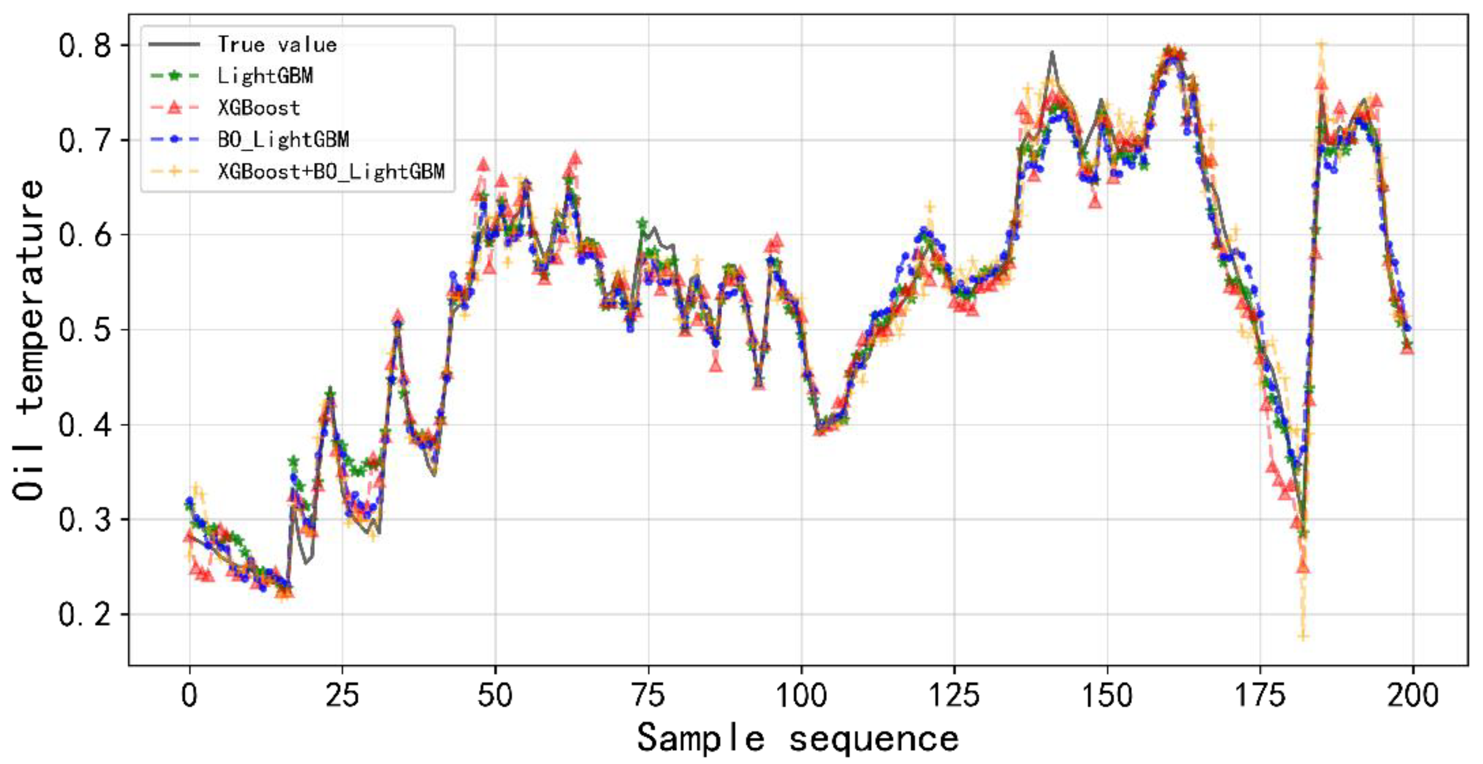Figure 6 shows the prediction result curve for each model.

In order to prove the correctness and validity of the proposed method for condition monitoring of offshore wind turbine gearboxes, the predicted value of the combined model is compared with the real value of the oil temperature of the gearbox in the first time period, and the accuracy of the oil temperature prediction model proposed in this paper is thus obtained before the adaptive threshold is then brought in to check whether the model is effective. The specific idea is to first predict the value of the combined model in terms of the predicted value of period one, with the true value of the gearbox’s oil temperature being the difference from the obtained the prediction residual. The residual sequence is then smoothed and the rate of change and standard deviation are calculated and finally brought into Formula (20) to obtain the adaptive threshold. In this article, the smoothing coefficient alpha is selected as 0.1, and the window sampling length is 2000. The threshold result is plotted as a gearbox operating condition monitoring diagram of period one, as shown in Figure 7.

As shown by the green circles in Figure 7, the residual crossing points are 507~522, 549~590, 694~697, 1095, and 1982. Among them, 1095 and 1982 exceeded the limit to a small extent and did not form a sustained violent vibration waveform, while 507~522, 549~590, and 694~697 showed three moments. The oil temperature of the gearbox of the wind turbine obviously exceeded the limit, and the duration was more than 2.5 h, which can allow us to preliminarily judge the operation status of the gearbox as abnormal at this time and issue an “alarm” signal. At both 1095 and 1982, the gearbox of the wind turbine unit issued an alarm signal. Combined with the actual fault handling report of the wind farm, the correctness and effectiveness of this verification method are verified.

In order to further illustrate the accuracy of adaptive thresholds for monitoring the oil temperature status of wind turbine gearboxes in this paper, $3\sigma$ is adopted to set constant thresholds for outlier monitoring. As can be seen in Figure 8, the constant threshold set by $3\sigma$ cannot reflect the trend in the oil temperature residual of the gearbox, which sets the threshold to three standard deviations above and below the mean. At moment 374, the residual exceeds the upper limit of the threshold, and the gearbox sends a false alarm signal.

The second period was selected as the research object of the condition monitoring method of the gearboxes of offshore wind turbines. During this time period, at the sampling point of about 500 moments, although the residual fluctuates the gearbox does not send an alarm signal because the alarm threshold is not crossed, as shown in Figure 9. Figure 10 shows the monitoring diagram of gearbox state period two with a constant threshold set by $3\sigma$, and the residuals at sampling points 371~374, 506, and 595 briefly cross the alarm threshold to trigger a false alarm signal. Combined with analysis of the gearbox operating state of period one and period two, the method proposed in this paper will not cross the alarm threshold in the face of a small sudden increase in residual values caused by the external environment, thereby reducing the probability of false alarms.

4. Conclusions

In this paper, taking the oil temperature of the gearboxes of offshore wind turbines as the prediction object, a combined prediction model based on IOWA operators is proposed. The effectiveness of the model is verified by a variety of regression evaluation indicators and compared with several prediction models in the existing literature, which proves that the combined prediction model proposed in this paper can further improve the accuracy of wind turbine condition monitoring. Finally, the predictions of the model were analyzed and compared with actual gearbox operating status data, which shows that the proposed model can accurately predict gearbox oil temperature failure.