Preliminary Multiphysics Modeling of Electric High-Voltage Cable of Offshore Wind-Farms

Abstract

During manufacture, handling, transportation, installation and operation, mechanical overstress can affect the electrical and thermal properties of the conductor. As the wires in general are made of copper, which is a very plastically deforming material, these stresses will gradually generate plastic deformations of the copper until the wires start to fail. The objective of this article is to study, by numerical modeling (using Comsol and Abaqus), the impact of damage mechanisms on the electrical and thermal properties of a submarine cable phase. The influence of plasticity and gradual copper wire failure on the physical behavior (electric and thermal) of the phase was assessed. The heat differences between a healthy conductor vs. a damaged one (either deformed plastically and/or with failed wires) derived from the numerical model may be an accurate indicator of the level of damage of wires, thus furthering advanced warning before being obliged to stop the exploitation because a mandatory heavy maintenance of the cables must be scheduled. Note that this can also be achieved by using an optical fiber as a sensor for structural health monitoring. This study will then make it possible to evaluate the impact of the modification of the resistance on the thermal behavior of the cable. All of these simulations will be carried out on one phase of a 36 kV 120 mm² copper submarine cable. Colloquially these are called “copper cables”, meaning cables with Cu conductors (120 mm² is the smallest conductor cross-section for array cables, which are usually 3-phase cables).

1. Introduction

The policy of the European Union has a carbon neutrality objective to achieve for 2050. In order to achieve this objective, it set itself a milestone for 2030 which consists of reducing greenhouse gas emissions by at least 55% [1], which is called “Fit for 55” by the EU Plan. One of the most promising European renewable energy sources is offshore wind energy, due to the tremendous potential of offshore wind farm projects that are ongoing and/or already in service either on the Atlantic Ocean or the North Sea. High-voltage electric cables for offshore farms are used for the transmission of high-voltage electric power between the wind turbines and the onshore station through a network of grids. It consists of a conductor (usually copper) and an insulator, the most efficient of which is Cross-Linked Polyethylene (XPLE). The cables have an insulation system consisting of layers of insulators, semi-conducting layers and a metal shield. Whatever the type of cable and the underlying applications, the insulation (XPLE) must in no case be damaged under parasitic mechanical stresses during manufacturing, handling and seagoing operations, or under high voltage electrical loading. The effects of ozone produced by electrical discharges in the air or from the path are also major sources of problems for these cables.

During manufacturing, handling, transport and seabed installation, high-voltage power cables for offshore can be overloaded, thus affecting their mechanical performances as well as their electric and thermal properties. Indeed, due to the multiple operations mentioned, copper wires of the conductor are subjected to complex loadings (tensile and torsion, compressive and tangential forces, etc.) that generate inter-wire friction. As the wires in general are made of copper, which is a very weak material, these stresses will gradually develop plasticity into wires, thus gradually leading to their failures. These plastic deformations are due to the formation, multiplication and displacement of mobile linear defects (dislocations) within the crystal lattices of the metal [2], which act as barriers to the transport of electrical charges. The movement of existing dislocations as well as the creation of new ones, therefore, changes the mechanical behavior of the metallic material, but also changes its physical properties (electrical, thermal, etc.). A great deal of research has been devoted to the aging of high-voltage power cables, and several facets were studied; especially the aging of XPLE by water-trees, structural health monitoring by way of embedded fiber-optic sensors to assess plasticity of copper, and how mechanical loading beyond the elastic limit also defines the “elastic limit” for both electric and thermal behaviors [2,3,4,5,6,7,8,9].

The objective of this article is to study, by numerical modeling under Comsol [10] and Abaqus [11], the impact of damage mechanisms on the electrical and thermal properties of an underwater power cable. Firstly, this study aims to assess whether the overload undergone by an underwater high-voltage power cable has a significant influence on the deterioration of its electrical resistance. This study will then make it possible to evaluate the impact of the modification of the resistance on the thermal behavior of the HV power cable. It is worthwhile to note that one of the originalities of the current article is that the model considers a multilayer conductor (1 + 6 + 12), with a length of 1 m along with considering the plasticity of copper. This article is looking at the cables from a multiphysics perspective, which includes mechanical, electrical and thermal behaviors. The multiphysics approach is dictated by multiphysics parameters which play central roles simultaneously. It is also interesting to note that the situation is worsened when one also considers the chemical and environmental aspects (salt, humidity, stress-corrosion, etc.) that are not assessed by the current article. The first part of this work therefore consists in considering the deformed geometry of the conductor in the elastoplastic domain as well as the non-homogeneous distribution of the electrical conductivity within a wire. The study will continue with analyzing their influence on the electrical resistance of the conductor. In the second part, the impact of the modification of the electrical resistance on the thermal behavior of the cable will be assessed. All of these simulations will be carried out on one phase of a 36 kV 120 mm² copper submarine cable. Before developing these two parts, we briefly present in the following section the design of the cable used in these simulations.

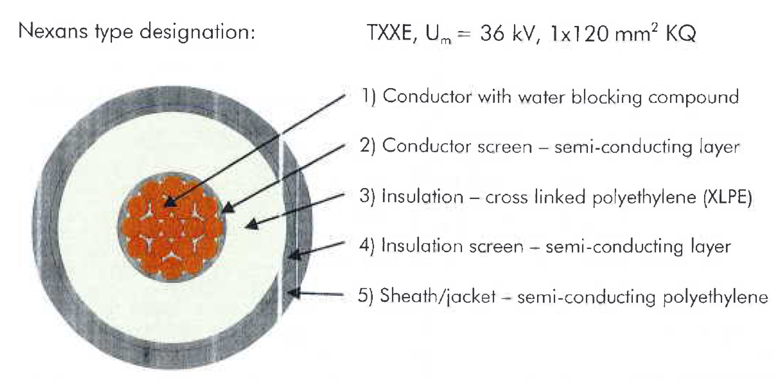
1.1. Cable Design—Preliminary Notions

The cable targeted by these simulations is a phase of a synthetically insulated (XLPE) [12] kV three-core cable. The phase conductor is made of copper with a section of 120 mm². The structure of the cable cross-section is shown in Figure 1 [12].

The geometric, thermal and mechanical properties of the cable constituents are presented in

Table 1. Geometric, thermal and mechanical properties of phase constituents and materials.

Component	Material	Young’s Modulus (GPa)	Poisson’s Ratio	Thermal Conductivity (W/k.m)	Volum Thermal Capacity [MJ.m-3 K-1]	Thickness (mm)
Conductor	Copper (Cu)	115	0.3	370.4	3.45	Diameter: 13
Semi-conductor	XLPE	0.34	0.34	0.28	2.4	1
Insulator (XPLE)	Cross-linked polyethylene (XLPE)	0.35	0.4	0.28	2.4	8
Sheath	High-density polyethylene (HDPE)	1.38	0.42	0.28	2.4	2.4

[12].

1.2. Numerical Model

In this section a mechanical model of an underwater cable conductor was built. This model reproduces the loading in tension that a submarine HV cable can undergo. This will allow us to calculate the distribution of the mechanical stresses and the deformation of the conductor. The deformation of the conductor will be used in an electrical model in the second part to calculate the electrical resistance. Finally, in the third part we will study the impact of the modification of the electrical resistance on the thermal behavior of the cable. Using Comsol Multiphysics, two models of the conductor of length, L (modeled cable length is 210 mm), have been developed:

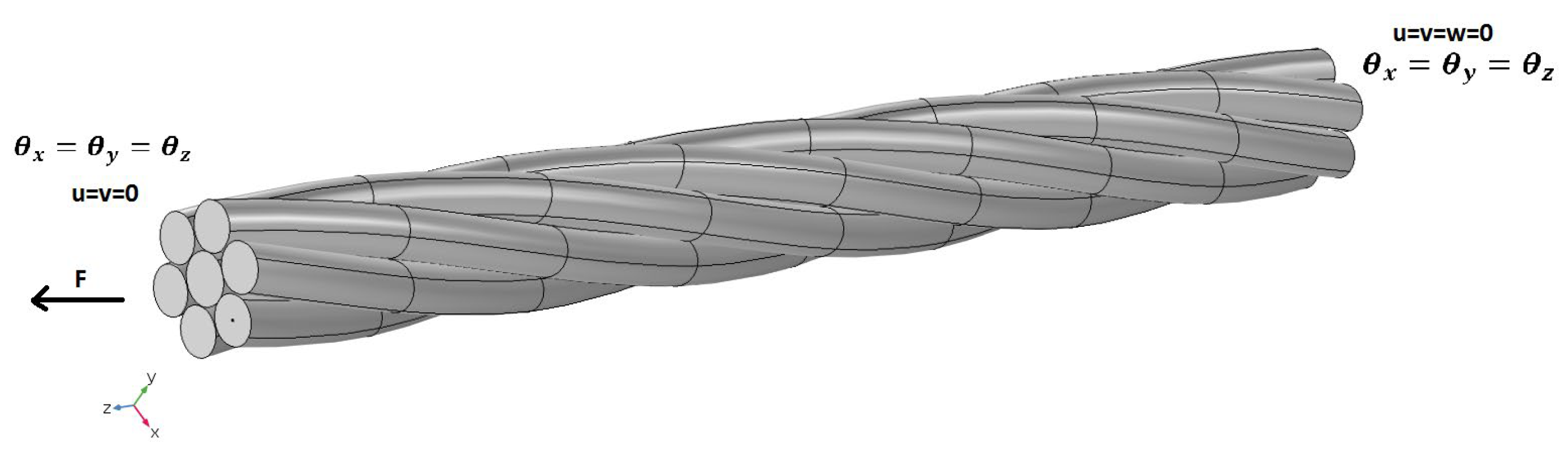
• A model of a 6-wire helical single-layer conductor with a central core (Figure 2).
• A second model of a bilayer conductor with 6 helical wires in the first layer and 12 wires in the second layer (Figure 3)

The characteristics of the geometry and material of the conductor (copper) are presented in

Table 2. Copper wire properties [4].

	Number	Radius `(mm)	Young’s Modulus (GPa)	Poisson’s Ratio	Unwounded (mm)	Elastic Limit (MPa)	Strength (MPa)	Electric Conductivity (S/m)
Central wire	1	1.97	115	0.33	************	135	340	5.9${10}^7$
Helical wire (1st row)	6	1.865	115	0.33	210	135	340	5.9${10}^7$
Helical wire (2nd row)	12	1.865	115	0.33	210	135	340	5.9${10}^7$

[1]:

For the meshes, quadratic elements are used. Figure 4 presents an example of the mesh used for the monolayer model. The mesh has 14,536 nodes for 54,252 elements.

Initially, with regard to the contact, the calculations carried out consider the hypothesis of a sticky contact. Studies in the literature show that the hypotheses on the contact have a negligible influence on the global behavior of the cable in tension, but they modify in a very important way the behavior in bending [13]. To take into account the plasticity of copper we have considered the stress–strain relationship shown in the previous paragraph. To analyze the results obtained, we calculate the Von Mises stress to position ourselves with respect to the elastic limit σ_e [14]. The Von Mises criterion is a criterion used in the field of the resistance of materials; metals in particular (but also for other materials, as well). It makes it possible to know, under given stresses, if a part deforms plastically or if it remains in the elastic domain. A ductile material begins to yield when Von Mises stress reaches a level equal to the stress limit. In most cases, the yield stress σ_e is used as the stress limit. Von Mises stress is given by the following equation:

$${\sigma }_{Von\_mises}=\frac{1}{2}\sqrt{{\left({\sigma }_1-{\sigma }_2\right)}^2+{\left({\sigma }_1-{\sigma }_3\right)}^2+{\left({\sigma }_2-{\sigma }_3\right)}^2}$$

(1)

where ${\sigma }_1,{\sigma }_2\mathrm{and}{\sigma }_3$ are the main stress components. Plasticity starts when ${\sigma }_{Von\_mises}\ge {\sigma }_e$.

2. Results and Discussion

We simulated the behavior of the cable for a monotonic tensile force ranging from F = 0 to F = 25 kN. The results corresponding to the total displacement of the cable are given in Figure 5. The distribution of Von Mises stress is shown in Figure 6 and Figure 7.

From the figures below one can note that the stresses are significant at the level of the central wire as well as in the contact zones between the latter and the helical wires.

In the next section, the deformation of the conductor resulting from the mechanical calculations will be imported into the electrical model to calculate the electrical resistance, the objective being to understand the influence of the elastic–plastic deformation on the electrical behavior of the conductor.

2.1. Finite Element (EF) Model

DC electrical simulations are performed using the electrical module of the Comsol software. The model developed consists in subjecting the deformed structure obtained by the mechanical study to an electric potential difference between the two extreme surfaces of the conductor, as depicted in Figure 8.

The DC electrical model is governed by the charge conservation equation:

$$\left\{\begin{array}{c}div\left(\mathrm{J}\right)=0\\ \mathrm{J}=\sigma \mathrm{E}\\ \mathrm{E}=-\nabla \mathrm{V}\end{array}\right.$$

(2)

where J (A/m²) is the current density, E (V/m) is the electric field, V (V) is the electric potential and σ(S/m) is the electric conductivity of the material. This model makes it possible to calculate the electrical potential, V. We will also consider the impact of the mechanical stresses symbolizing the work hardening that could exist and its effect on the electrical conductivity of the material. For this, we will introduce an experimental behavior law [15] obtained for a copper wire coupling the electrical conductivity and the mechanical stresses. This law would make it possible to control the evolution of the electrical conductivity according to the distribution of the stress resulting from mechanical calculation (Figure 9).

Note that computation of the current intensity (I) in the of conductor was obtained by making the cut plane 2D at the middle cross-section of the cable and using the surface integral over current density (Jz) along the z-axis.

I = ∬ Jzds

(3)

The electrical resistance of the conductor can be calculated by Ohm’s law: R = ΔV/I.

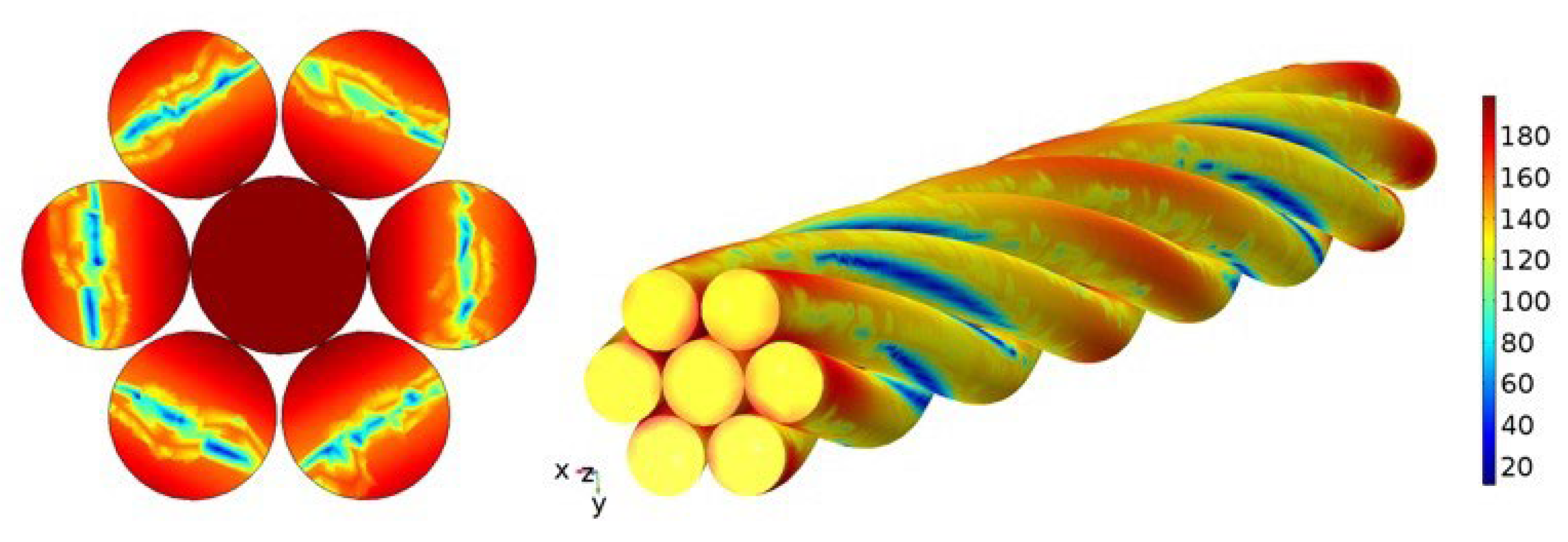
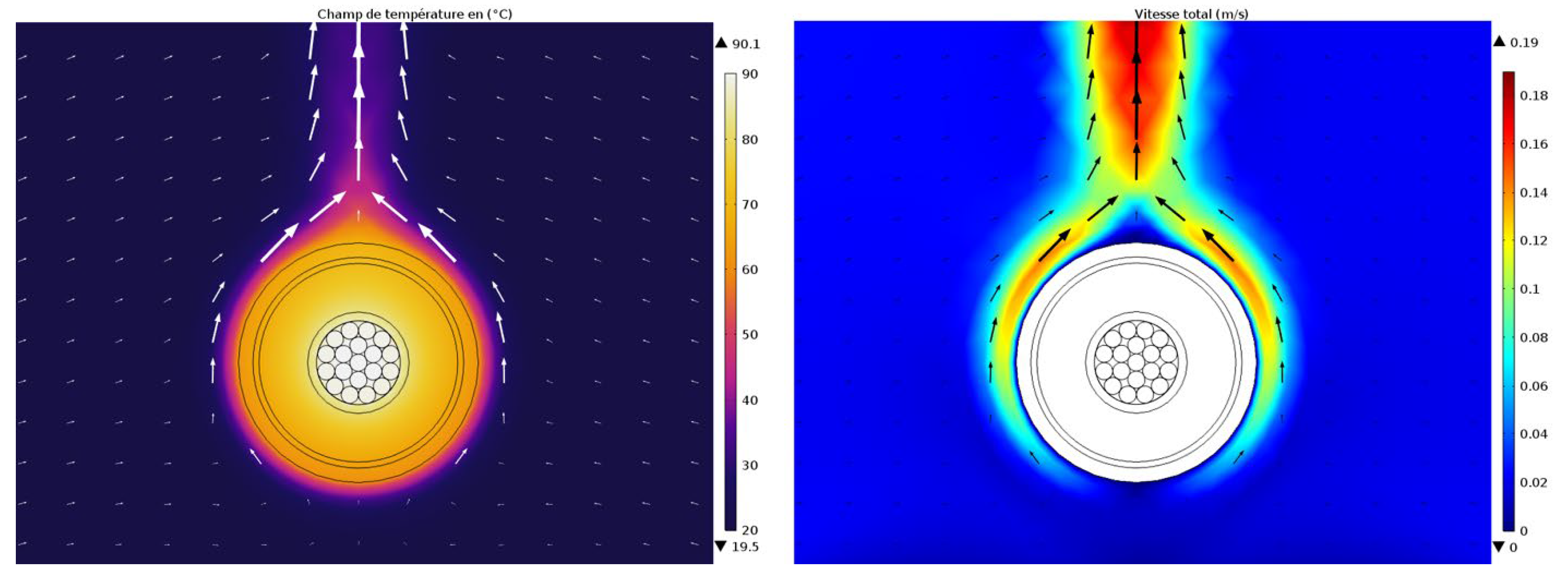
2.2. Numerical Results

In order to test the model, it was applied to a copper wire. Indeed, we have an analytical solution which connects the variation of resistance to the deformation for the case of a cylinder loaded under tension (Figure 10). This analytical validation would make it possible to test the numerical results and therefore that of the model before embarking on the more complex case of the complete conductor, which will be impossible to verify.

The electrical resistance of a cylinder is given by the relation R = ρL/S, where ρ is the resistivity of the material, S is the area of the base and L its length. The variation of the resistance of a cylinder loaded in tension, in the plastic area [16], is given by the following equation:

$$\frac{\Delta R}{R}={\left(1+\epsilon \right)}^2-1$$

(4)

where ε is the total strain. To validate the numerical model, we consider a copper cylinder with a radius of 0.1 mm and a length of 1 mm. Figure 11 presents the resistance variation obtained numerically and analytically. The figure shows a good agreement between the numerical model and the analytical solution. We can therefore apply our numerical model to the conductor 1 + 6 and 1 + 6 + 12.

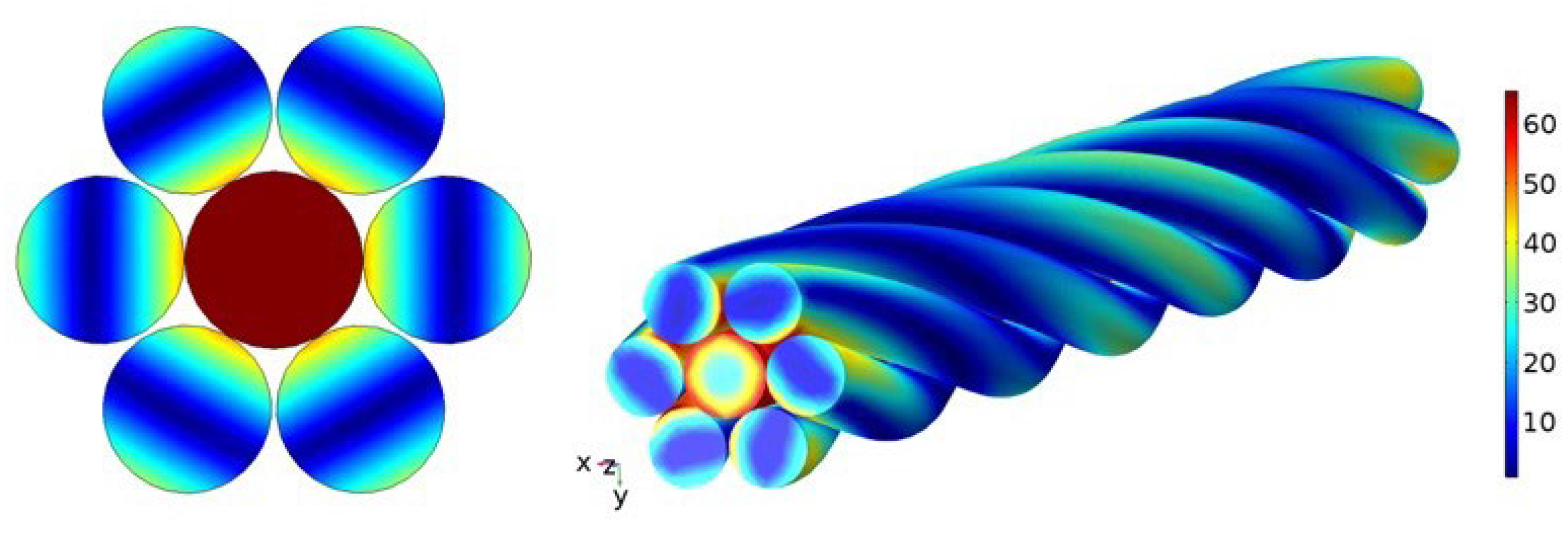
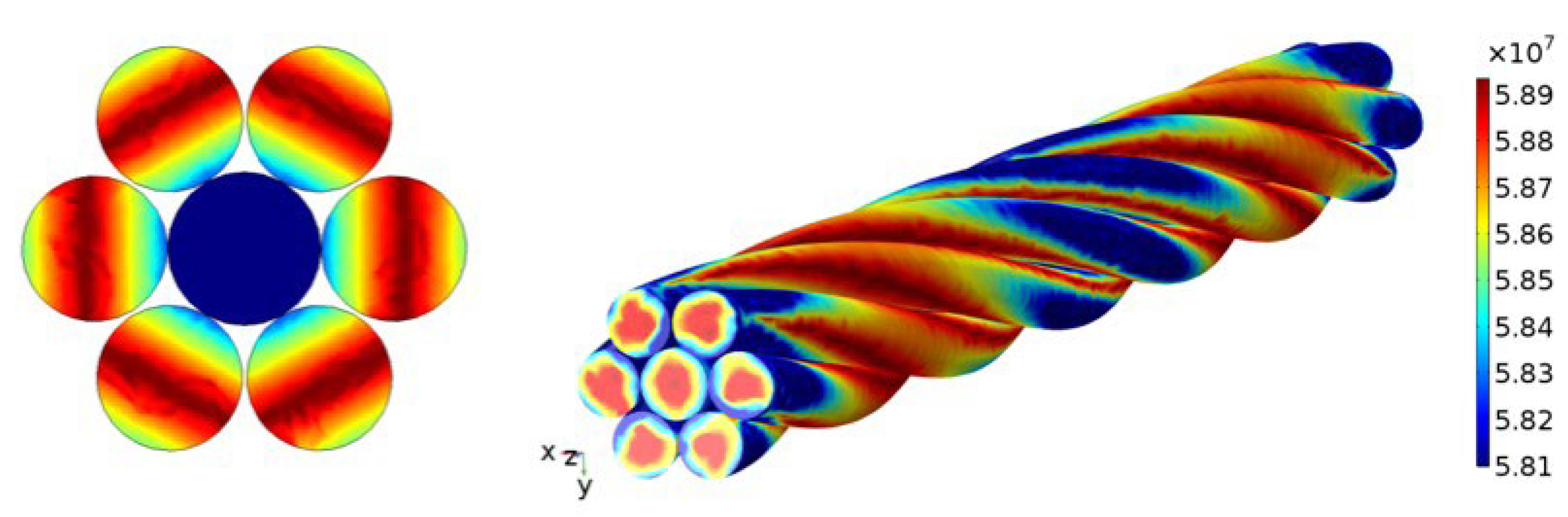
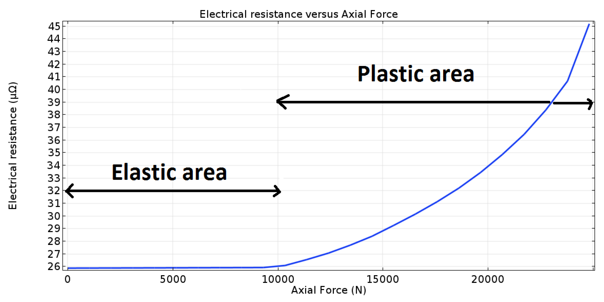
2.3. Conductor Geometry Type 1 + 6

Figure 12 shows the distribution of Von Mises stress over the conductor in the plastic area, and its correspondence in electrical conductivity is depicted in Figure 13.

From these figures, it can be seen that the electrical conductivity is lower in the areas where the mechanical stress is greater. This means that these areas are less conductive.

Figure 14 shows the density of volume losses by Joule effect for a conductor, both without and with mechanical constraints. It can be seen in the figure on the right that the losses are uniform and are approximately $3·{10}^5 \mathrm{W}/{\mathrm{m}}^3$. On the left figure, one notices a non-homogeneous distribution of the losses, which corresponds to the distribution of the mechanical stresses. Indeed, in the zones where the mechanical stresses are important, the losses by Joule effect are also important.

The total resistance is determined by integrating the current density over the cross section of the structure. The resistance is therefore calculated by Ohm’s equation:

$$R=\frac{\Delta V}{I}$$

(5)

Figure 15 shows the evolution of the total electrical resistance of the conductor as a function of a monotonic loading. From this figure, the resistance is almost constant in the elastic region. In the plastic area, an increasing evolution of electrical resistance is noticed. For example, for a load of 20 kN the resistance has increased by 30% ($\frac{\Delta R}{R}$).

To reduce the cost of calculations in time and memory, we will carry out a study of the sensitivity of the electrical resistance when only a portion of the conductor is modeled. Figure 16 shows the evolution of the electrical resistance variation for 1/10th and 1/4th of a step as a function of the average stress in the conductor. The curves of the evolution of the variation of electrical resistance for the different portions of the pitch are almost identical with a slight difference for the case of a pitch of 2%. As a result, the rest of the simulation will be conducted on 1/10th of a step.

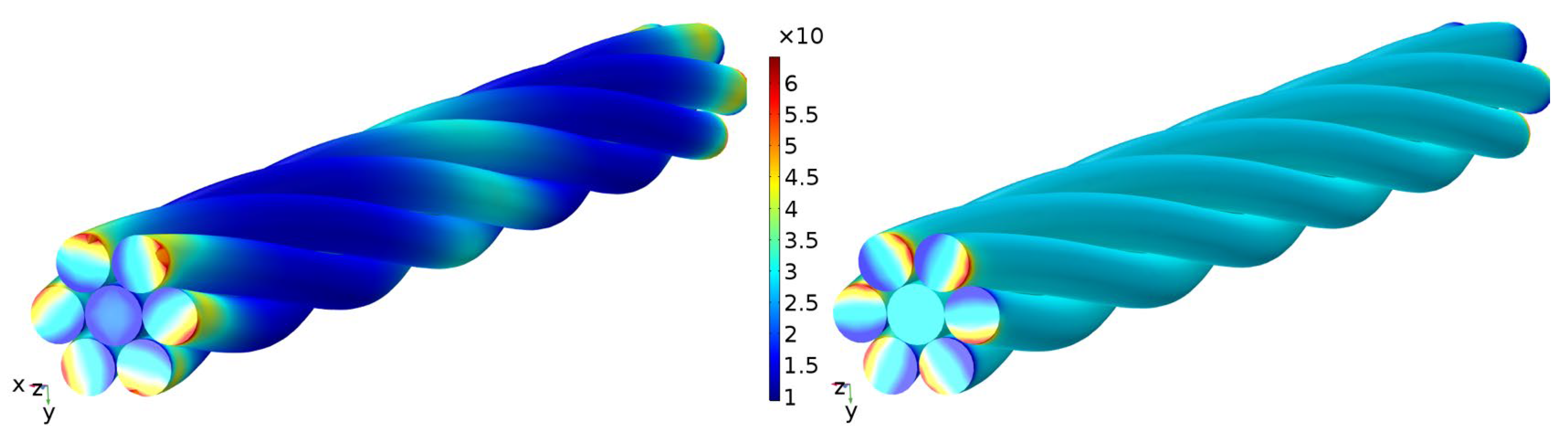
2.4. Conductor Geometry Type 1 + 6 + 12

For important calculation times, one models only 1/10th of the step of winding in order to limit the size of the mesh. Figure 17 shows the distribution of Von Mises stress in the conductor as well as the distribution of the electrical conductivity. Figure 18 shows the influence of plasticity on the behavior of the electrical resistance of the conductor. It can be seen that the electrical behavior of a two-layer conductor (1 + 6 + 12) has the same tendency as a single-layer conductor.

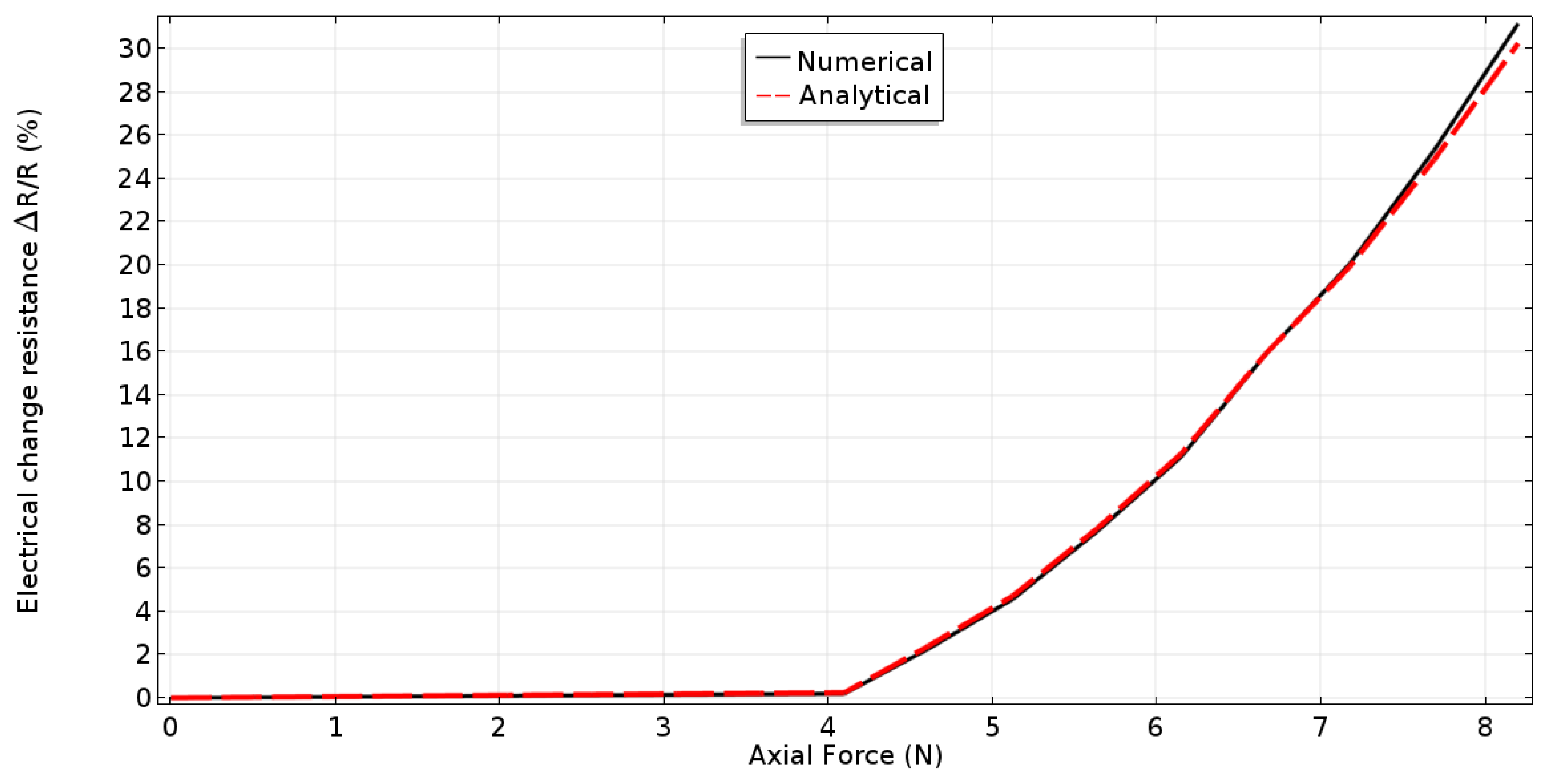
2.5. Influences of Some Variables on the Electrical Resistance of the Conductor

In this section, the impact of some parameters such as friction, step length and progressive wire failure on the electrical behavior of the conductor, are studied.

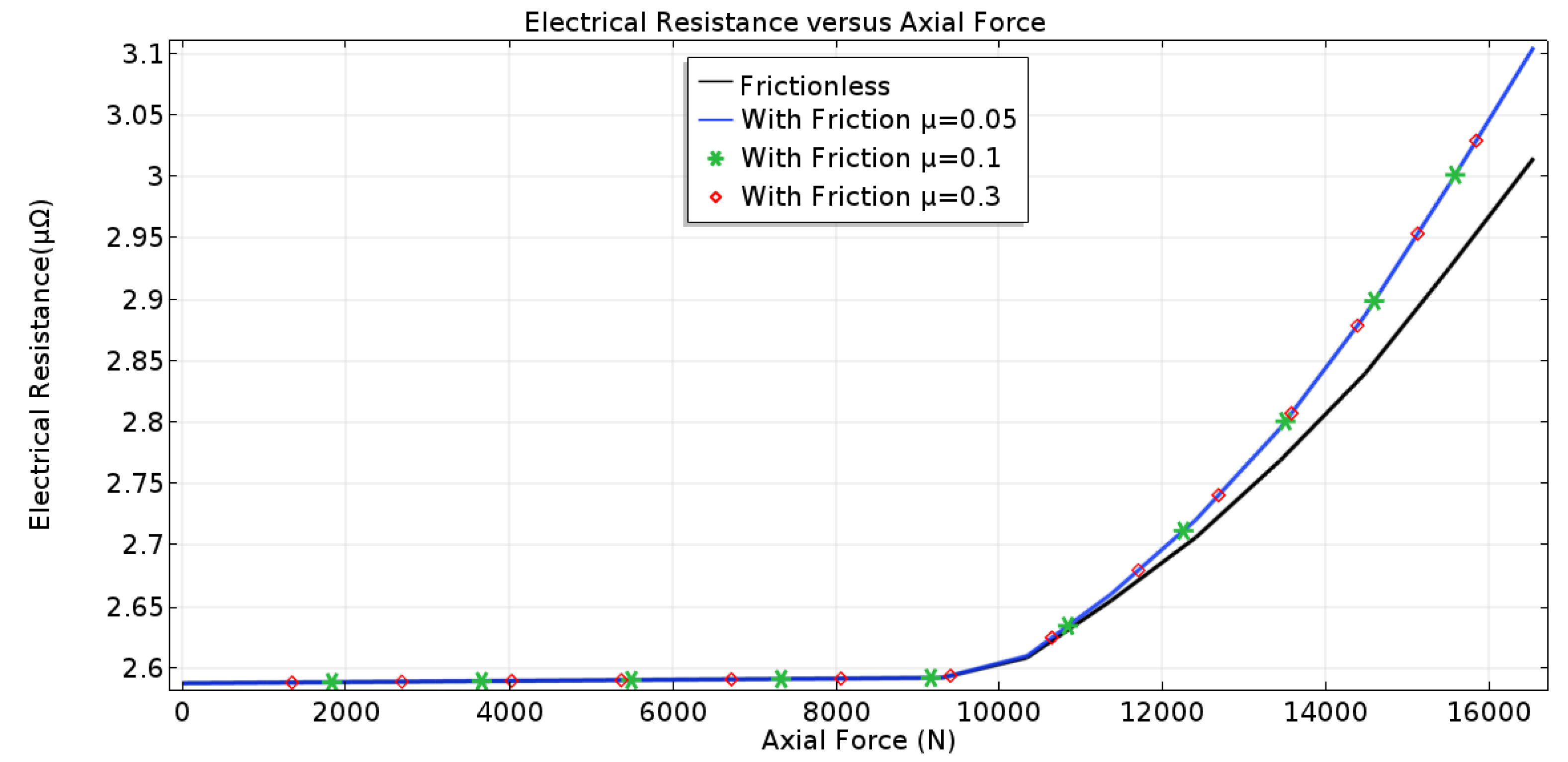
2.6. Effect of Friction

The consideration of the contact is managed by an algorithm of the surface-to-surface type. Only radial contact is considered, admitting the hypothesis of non-contact between wires of the same layer. Figure 19 shows the evolution of electrical resistance as a function of loading for different values of friction coefficient, µ. It can be seen that the impact of friction is almost zero in the elastic domain and that it remains very low in the plastic region.

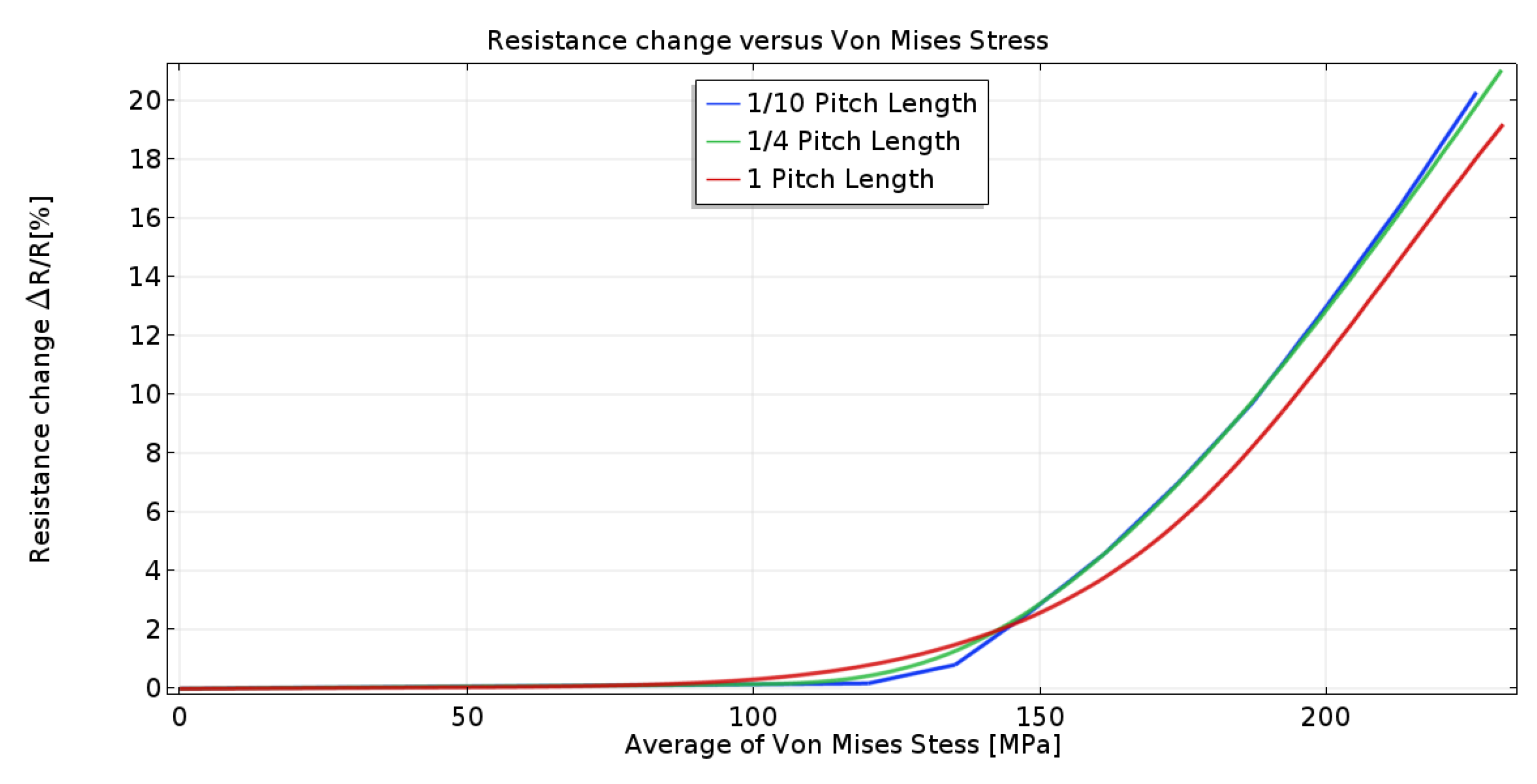
2.7. Pitch Length Effects

Figure 20 shows the variation of the electrical resistance versus the mechanical loading. As shown, the variation of the resistance decreases when the pitch length increases; then it no longer varies. From the numerical results, it is clear that the electrical resistance of low-pitch conductors is very high, which leads us to advise against them. Due to their low tensile stability, low torsional stiffness and low bending strength, smaller pitch length conductors are more advantageous. Therefore, one has to choose a pitch with an acceptable electrical resistance, torsional rigidity and bending resistance and which respects the constraints imposed on the conductor.

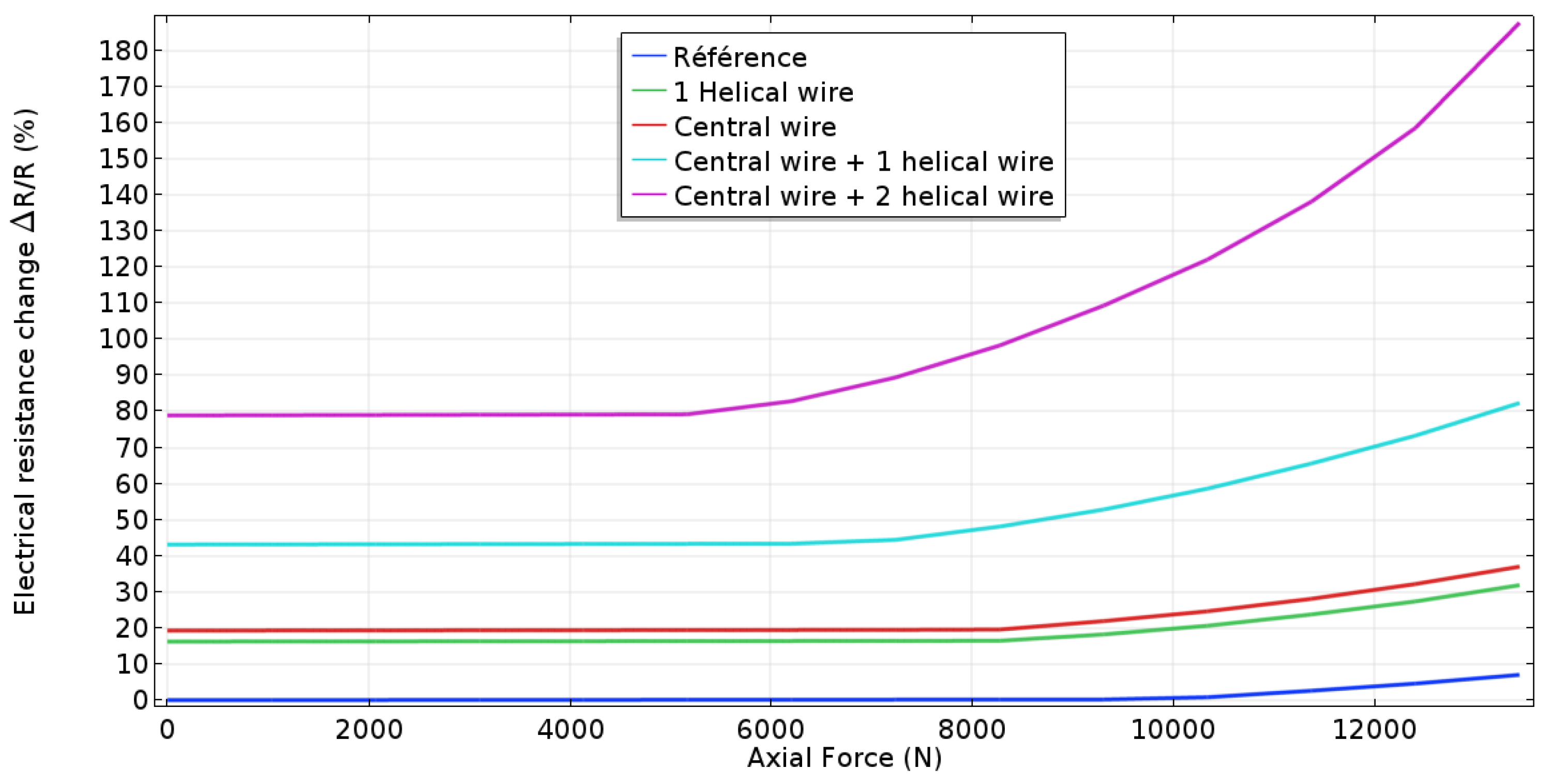
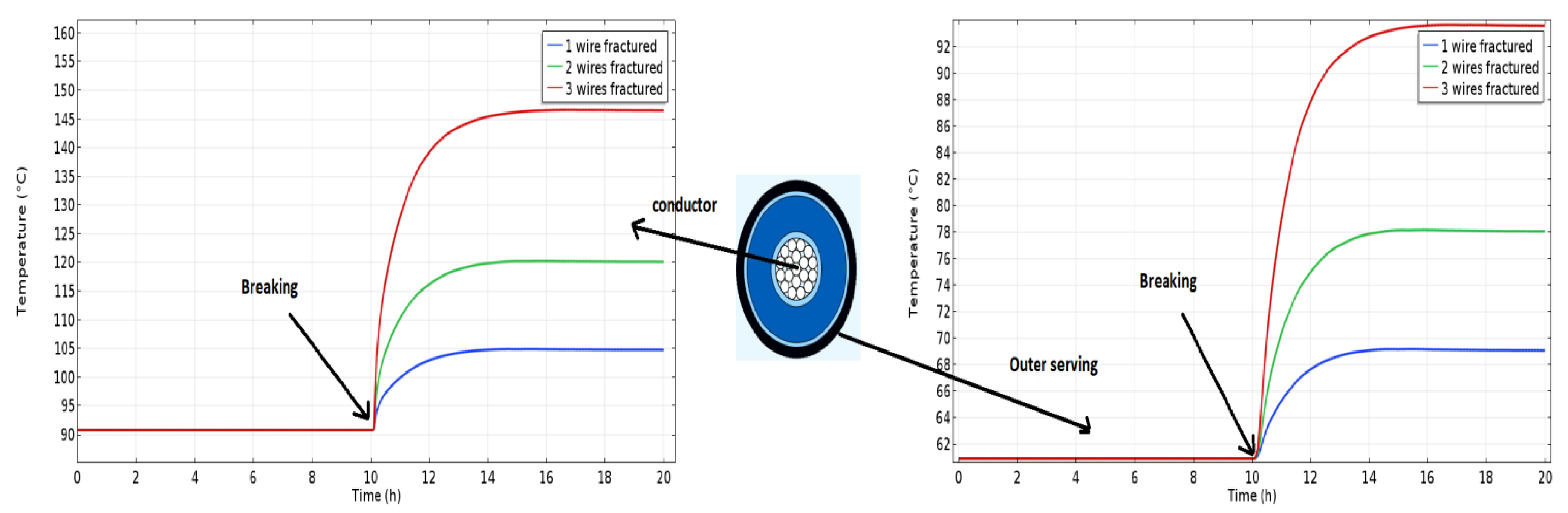
2.8. Effects of Progressive Wire Failure

Figure 21 and Figure 22 show the effect of progressive conductor wire failure on electrical resistance and resistance variation. It can be seen that the impact of wire breakage is very significant on the electrical resistance. In the field of elasticity, we notice an increase ranging from 20% for one cut wire to 80% for three cut wires. This shows that the mechanical behavior of the conductor influences its electrical behavior.

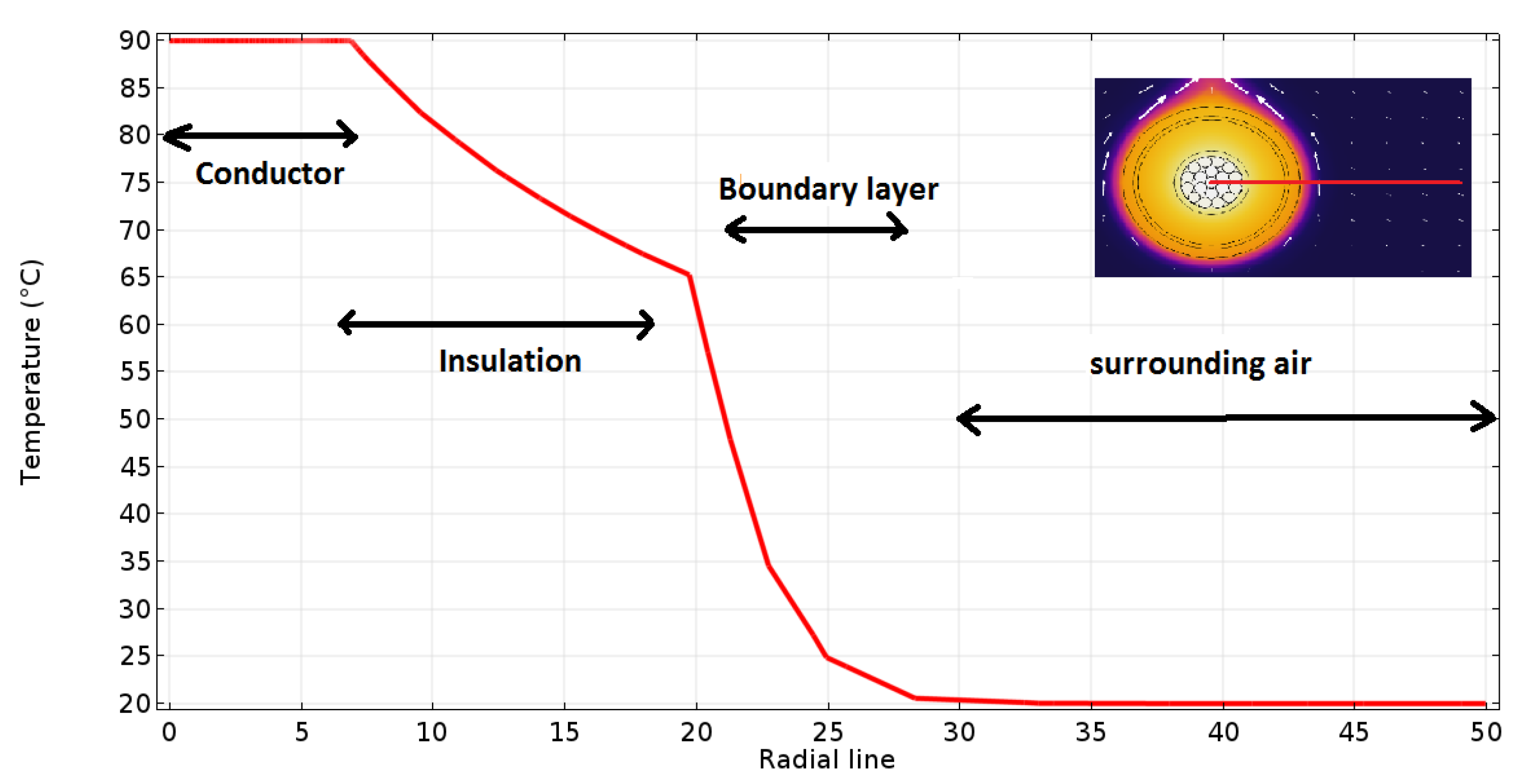
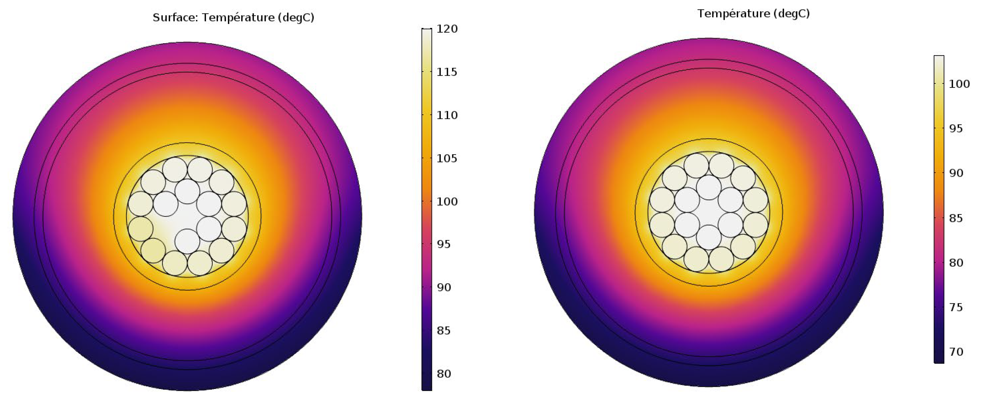
2.9. FE Thermal and Thermoelectric Modeling

In this section the thermal behavior of the cable, considering the mechanical effects on the electrical resistance of the conductor studied in the previous section, is assessed. A thermal model under natural convection, allowing the calculation of the distribution of the temperature in the section of the cable, is first built. To calculate the temperature distribution inside and on the boundary of the calculation domain (the latter corresponds to the section of the studied phase), the equation of heat transfer by conduction in unsteady state considering the convection [17] is applied. It is defined as follows:

$$\rho C_p\frac{\partial T}{\partial t}+\rho C_{p}u·\nabla T+div\left(-K\nabla T\right)=Q$$

(6)

where T is the absolute temperature (K), K is the thermal conductivity (W·m⁻¹·K⁻¹), Q is a heat source (W·m⁻³), u is the velocity field of the fluid (m/s), $\rho \left(\mathrm{kg}/{\mathrm{m}}^3\right)$ is the volume weight, and $C_p\left(\frac{J}{kg.K}\right)$ is the calorific capacity. Under natural convection, the velocity field is created by the temperature field, and the velocity obeys the Navier–Stokes equations [17]:

$$\left\{\begin{array}{c}div\left(u\right)=0\\ {\rho }_0\frac{\partial u}{\partial t}+{\rho }_{0}u·\nabla u=-\nabla p+\rho g+\mu {\nabla }^{2}u\end{array}\right.$$

(7)

where ρ is the density. It depends only on the temperature and is given by the Boussinesq approximation $\rho ={\rho }_0\beta \left(T-T_0\right)$, where $T_0\mathrm{and} {\rho }_0$ are the parameters relating to the fluid, β is the coefficient of expansion at constant pressure, p is the pressure (Pa) and µ is the dynamic viscosity coefficient of the air. For the heat sources, Q, we will consider that generated in the conductor by the Joule effect [18]:

$${\mathrm{W}}_{\mathrm{c}}=I_c^2.R_{Ac}$$

(8)

$R_{AC}\left(\mathrm{W}/\mathrm{km}\right)$ is the cable resistance and $I_c\left(\mathrm{A}\right)$ is the current density of the conductor. The cable is considered laid horizontally, in air with an ambient temperature of 20 °C.

The idea behind thermal sizing of the phase is to enable electric current transport without exceeding the maximum heat allowed by the cable, which is 90 °C (upper limit for XPLE insulator thermal resistance). The suggested model will help figure out the effects of plasticity and wire gradual failure on the thermoelectric performance of the cable. A 2D model was developed just to save calculation time. Heat transfer by steady state conduction when considering thermoelectric coupling is as follows [19]:

div(−K∇T) = σ.|∇V|2

(9)

T is the temperature (K), K is the thermal conductivity (W∙m⁻¹∙K⁻¹), V is the electrical potential (v), and σ(S/m) is the electrical conductivity of the material, given by the following:

σ = L/RA

(10)

R is the conductor resistance, A is the total surface area of the wire, and L is its length. Natural convection and heat radiation were considered on the phase surface in such a way as to enable the defining of the corresponding boundary conditions as follows:

−∇(KT)·n = h(Text − T)

(11)

where h is the convective heat transfer coefficient, and T_ext is the ambient temperature. The h parameter at the surface is calculated from h = k·Nu/L (L is the cable’s diameter, k is the contour’s thermal conductivity and Nu is the Nusselt number). Under natural convection, and in the event that the phase is placed horizontally, the Nusselt number is [19,20]

Nu = (0.6 + 0.387 × R^1/6a / (1 + (0.559Pr)^9/16)^8/27

(12)

Using the Stefan–Boltzmann law, the heat radiation on the cable surface is as follows:

−∇(KT)·n = εv(T⁴ext − T⁴)

(13)

where ε is the emissivity, taken as 0.9, and ν is the Stefan–Boltzmann constant.

Figure 23 illustrates the cable environment as well as the boundary conditions considered. At the borders, it is assumed that no heat exchange can occur, which is translated by a zero normal flux. The free circulation of air on the borders (zero pressure) is assumed. To reach a temperature of 90 °C in the conductor with the conditions defined above, we are going to circulate an admissible current which is equivalent to 515 A. The value of the maximum intensity of the current, I, admissible (A) in the permanent mode for a cable HVAC is given in the IEC standards [18] by the following equation:

$${\mathrm{I}}_{\mathrm{admissible}}={\left[\frac{\Delta \theta -W_d\left[0.5T_1+n\left(T_2+T_3+T_4\right)\right]}{R_{ac}{T}_1+n{R}_{ac}\left(1+{\lambda }_1\right)T_2+n{R}_{ac}\left(1+{\lambda }_1+{\lambda }_2\right)\left(T_3+T_4\right)}\right]}^{0.5}$$

(14)

where:

• $\Delta \theta ={\theta }_{max}-{\theta }_a$;
• ${\mathrm{W}}_{\mathrm{d}}$ are the dielectric losses in the insulator;
• $\mathrm{n}$ is the conductor wire number;
• $R_{ac}$ is the resistance of the conductor to an alternative current;
• ${\mathsf{\lambda }}_1$ is the dissipation factor of the screen;
• ${\mathsf{\lambda }}_2$ is the dissipation factor in the shield.

The electrical resistance of the reference conductor is 0.153 $\mathsf{\Omega }/\mathrm{km}$.

Figure 23. Effects of the environment geometry of the cable and imposed boundary conditions.

Figure 23. Effects of the environment geometry of the cable and imposed boundary conditions.

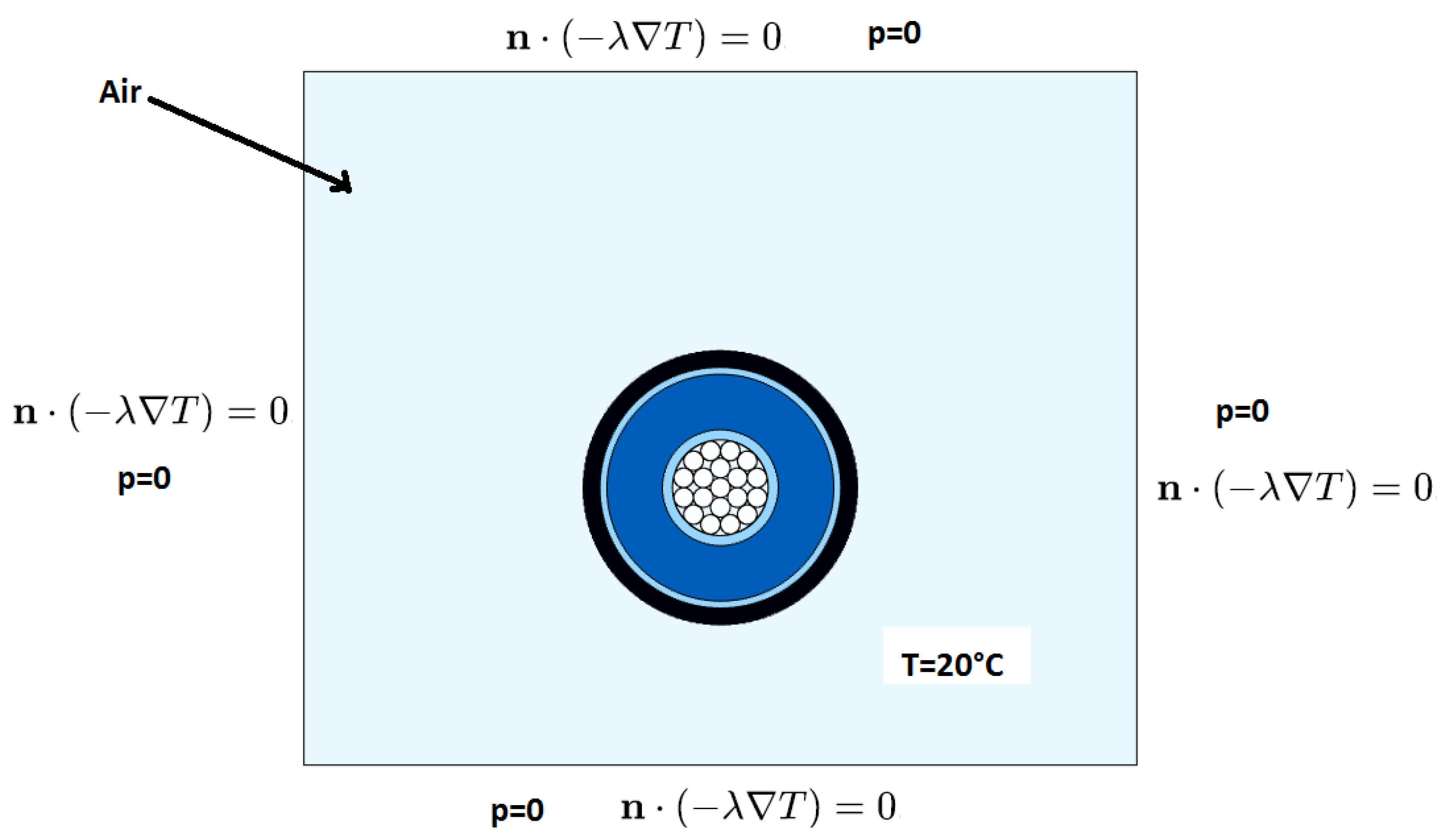
2.10. Numerical Results

Figure 24 shows the distribution of the temperature field (left) and the air velocity field (right) of the cable in equilibrium, obtained numerically. The arrows illustrating the velocity field are shown in both figures. To visualize the temperature variations in the various constituents of the cable, the temperature profile is drawn along a radial section starting from the conductor (Figure 25).

Table 3. Mean temperature in the cable.

Constituents	Mean Temperature (°C)
Conductor	89.94 °C
Semi-conductor layer	82.79 °C
XPLE	71.29 °C
Semi-conductor layer	64.53 °C
Sheath	62.30 °C

summarizes the average temperature in each component of the cable.

These results will serve as a reference for the next experiment. Indeed, when the cable undergoes mechanical stresses, we expect an impact on the thermal behavior.

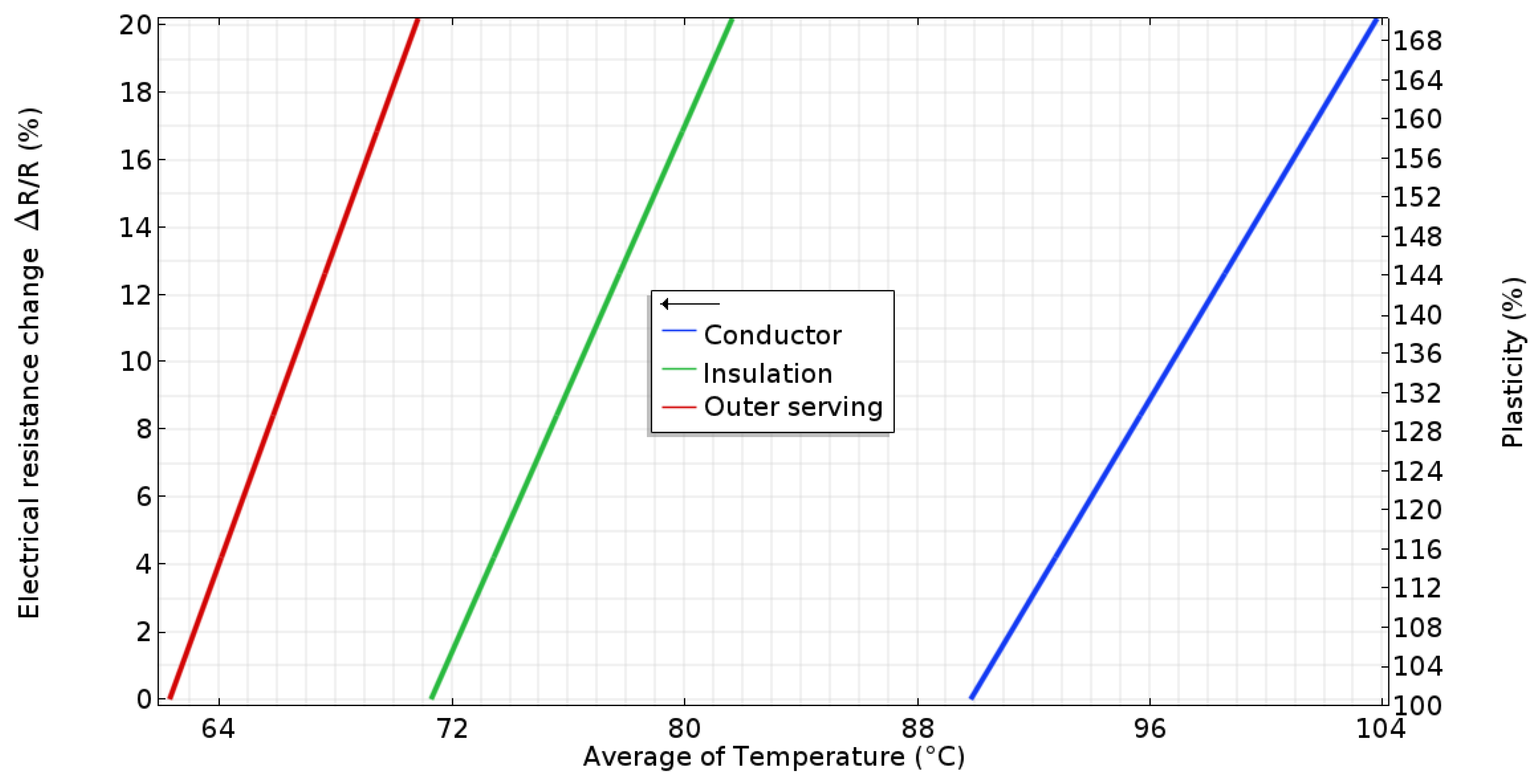
2.11. Copper Plasticity Effects on the Cable Temperature

In this section, we study the impact of conductor plasticity on cable temperature. For this, we consider several levels of work hardening ranging from 100% up to 168% of the elastic limit. Figure 26 shows the impact of plasticity on the thermal behavior of the cable. It is clear that the resistance increases with the increase in the rate of work hardening of copper.

The average temperature of the cable’s components versus copper plasticity levels is pictured in Figure 27, where it is clear that the temperature is quite a bit higher in the conductor compared to what happens in the XPLE.

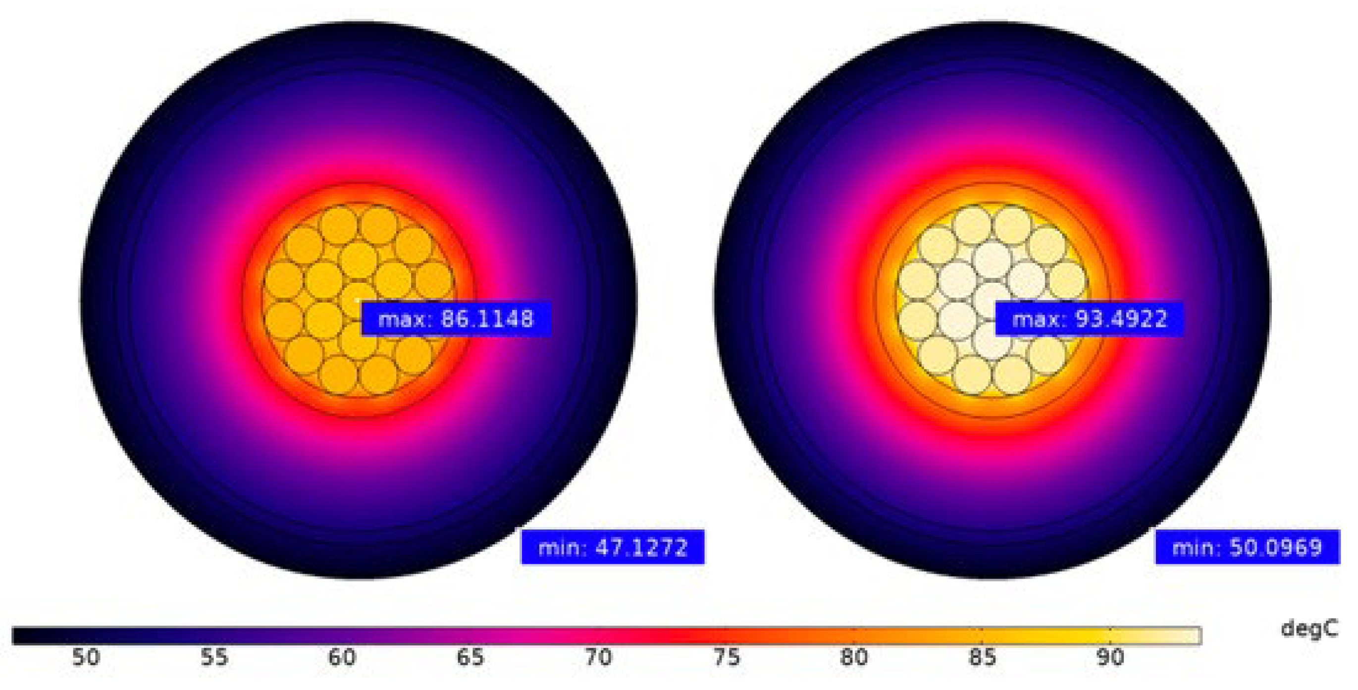
2.12. Effects of Wire Failures on Cable Temperature

In this section, we are interested in the impact of wire failure on cable temperature. Figure 28, Figure 29 and Figure 30 show the temperature distribution for one wire with up to three cut wires.

From these figures, one can notice an increase in temperature ranging from 16% for one cut wire to 60% for three cut wires.

Table 4. Mean temperature in the phase on safe and on several damaged conditions.

Constituents	Mean Temperature (°C) Central Wire Failure	Mean Temperature (°C) With Failure of 2 Wires	Mean Temperature (°C) With Failure of 3 Wires
Conductor	104.42 °C (+16.1%)	118.95 °C (+32%)	145.01 °C (+61%)
Semi-conductor layer	96.01 °C (15%)	109.23 °C (+31%)	133.03 °C (+60%)
XPLE	82.09 °C (+15%)	92.89 °C (+30%)	112.34 °C (+57%)
Semi-conductor layer	73.91 °C (+14%)	83.28 °C (+29%)	100.16 °C (+55%)
Sheath	71.21 °C (+14%)	80.11 °C (+28%)	96.15 °C (+54%)
Temperature variation $\frac{\Delta T}{T}\left(\%\right)$	14.8%	30%	57%

summarizes the average temperatures in the different constituents of the phases as well as the temperature variations generated.

With this multiphysics modeling, the various aspects pertaining to the use of high-voltage electric cables and their aging have been investigated. A clearer idea about the further assessment of their in-service performances can be envisaged through deepening the various aspects that have been addressed in this article. The originality of the suggested work is of the same inspiration as the previous research on strengthening large offshore wind-blades with carbon nanotube-reinforced bonding along with post-stitching [21].

As a perspective, it should be noted that the current article was conducted with basic multiphysics modeling, and a consequent bench of research is still to come. One particular source of trouble for high-voltage electric cables is partial discharge (PD). In a high-voltage electric cable, when an insulation defect exists, it can be the cause of a partial electric discharge. This discharge occurs through part of the insulation and not over its entirety. It is important to note that the electrical discharge of high-voltage cables is subject of numerous tests whose aim is to locate the discharge before it leads to a major failure, knowing that the discharge once initiated will cause and, especially, will increase in intensity until the major failure of the insulation [22]. It is also important to note the pernicious nature of the PD, as it is a mechanism that generates progressive damage over time and therefore acts by significantly lowering the durability of high-voltage cables. Therefore, special attention is paid in several high-tech industries, in particular aeronautics, to the long-term effects [23]. More specifically, when the voltage between the deep conductor and the insulator is very high, the susceptibility to partial discharge is increased. A number of tests and standards have been developed to test the effects of PD when cables are subjected to high voltage [24,25]. As a future direction of research, we plan to extend our model in order to numerically simulate the PD. We are also planning a coupling between long-term mechanical fatigue tests on the cable with placing the phases under high electrical tension. The experimental multiphysics coupling that we plan would make it possible to obtain additional results in order to consolidate the models presented in this work. It is worthwhile to note that valuable recommendations relating to the mechanical testing of power cables have been published (see for example [26]).

3. Conclusions

High-voltage electric cables for offshore farms, by the nature of their constituent materials, their environments of use and their operations, will necessarily have aging kinetics of a multiphysical nature. It is on this first point that we wish to insist and that we have tried to develop in this article. FEM was used to model the influence of the plasticity of copper and the progressive ruptures of the wires of the conductor of the phase. The effects of these two mechanisms clearly show that with increasing mechanical damage, the mechanical, electrical and thermal behaviors undergo a continuous decrease, and their inter-relation is thus demonstrated. Environmental influences (humidity, salt, stress-corrosion, fatigue, etc.) should increase the impact of the aforementioned effects, and this would be a possible extension of this work.

The proposed models should be viewed as an introduction to better target the influential parameters and combine them to succeed in the future in setting up a more robust modeling of the multiphysical mechanisms that come into play during the tensioning of offshore, electrical, high-voltage cables. The quantitative side, although being crucial, is a secondary consideration in this study because the experimental values clearly show that the models allow us to obtain values consistent with what happens experimentally.

References

1. European Union Long-Term Strategy. Available online: https://energy.ec.europa.eu/topics/renewable-energy/renewable-energy-directive-targets-and-rules/renewable-energy-targets_en (accessed on 18 July 2023).
2. Ech-Cheikh, F. Numerical and Analytical Modeling of the Mechanical and Multi-Physics Behavior of High-Voltage Phase of Offshore Electric Cable. Ph.D. Thesis, Ecole Centrale, Nantes, France, 26 January 2022. [Google Scholar]
3. Matine, A.; Drissi-Habti, M. On-Coupling Mechanical, Electrical and Thermal Behavior of Submarine Power Phases. Energies 2019, 12, 1009. [Google Scholar] [CrossRef]
4. Drissi-Habti, M.; Raman, V.; Khadour, A.; Timorian, S. Fiber Optic Sensor Embedment Study for Multi-Parameter Strain Sensing. Sensors 2017, 17, 667. [Google Scholar] [CrossRef] [PubMed]
5. Drissi-Habti, M.; Raj-Jiyoti, D.; Vijayaraghavan, S.; Fouad, E.-C. Numerical Simulation for Void Coalescence (Water Treeing) in XLPE Insulation of Submarine Composite Power Cables. Energies 2020, 13, 5472. [Google Scholar] [CrossRef]
6. Miceli, M.; Carvelli, V.; Drissi-Habti, M. Modelling Electro-Mechanical Behaviour of an XLPE Insulation Layer for Hi-Voltage Composite Power Cables: Effect of Voids on Onset of Coalescence. Energies 2023, 16, 4620. [Google Scholar] [CrossRef]
7. Drissi-Habti, M.; Manepalli, S.; Neginhal, A.; Carvelli, V.; Bonamy, P.-J. Numerical Simulation of Aging by Water-Trees of XPLE Insulator Used in a Single Hi-Voltage Phase of Smart Composite Power Cables for Offshore Farms. Energies 2022, 15, 1844. [Google Scholar] [CrossRef]
8. Drissi-Habti, M.; Neginhal, A.; Manepalli, S.; Carvelli, V.; Bonamy, P.-J. Concept of Placement of Fiber-Optic Sensor in Smart Energy Transport Cable under Tensile Loading. Sensors 2022, 22, 2444. [Google Scholar] [CrossRef] [PubMed]
9. Drissi-Habti, M.; Neginhal, A.; Manepalli, S.; Carvelli, V. Fiber-Optic Sensors (FOS) for Smart High Voltage Composite Cables—Numerical Simulation of Multi-Parameter Bending Effects Generated by Irregular Seabed Topography. Sensors 2022, 22, 7899. [Google Scholar] [CrossRef]
10. Abaqus Software. Available online: https://www.3ds.com/fr/produits-et-services/simulia/produits/abaqus/ (accessed on 18 July 2023).
11. Comsol Multi-Physics Software. Available online: https://www.comsol.com/ (accessed on 18 July 2023).
12. Available online: https://www.nexans.com/en/markets/power-generation/offshore-wind/NorthWind.html (accessed on 18 July 2023).
13. IEC60287-1-1; Electric Cables—Calculation of the Current Rating—Part 1—1: Current Rating Equations (100% Load Factor) and Calculation of Losses—General. International Electrotechnical Commission: Geneva, Switzerland, 2006.
14. Neber, J.H.; Mcgratb, M.H. The calculations of the temperature rise and load capability of cable systems. In Proceedings of the AIEE Summer General Meeting, Montreal, QC, Canada, 24–28 June 1957; Volume 76, pp. 1752–1772. [Google Scholar]
15. Napieralski, P.; Juszczak, E.N.; Zeroukh, Y. Nonuniform Distribution of Conductivity Resulting from the Stress Exerted on a Stranded Cable During the Manufacturing Process. IEEE Trans. Ind. Appl. 2016, 52, 3886–3892. [Google Scholar] [CrossRef]
16. Bonnet, A.M. Analyse des Solides Déformables par la Méthode des Éléments Finis; Ecole Polytechnique: Palaiseau, France, 2007. [Google Scholar]
17. Francesco, F.; Luca, M. Mechanical modeling of metallic strands subjected to tension, torsion and bending. Int. J. Solids Struct. 2016, 91, 1–17. [Google Scholar]
18. Liu, D.-S.; Ni, C.-Y. A thermo-mechanical study on the electrical resistance of aluminum wire conductors. Microelectron. Reliab. 2002, 42, 367–374. [Google Scholar] [CrossRef]
19. Long, C. Essential Heat Transfer, 1st ed.; Longman: London, UK, 1999. [Google Scholar]
20. Cable IEC Standards. Available online: https://www.elandcables.com/fr/electrical-cable-and-accessories/cables-by-standard/iec-cable (accessed on 18 July 2023).
21. Raman, V.; Drissi-Habti, M. Numerical simulation of a resistant structural bonding in wind-turbine blade through the use of composite cord stitching. Compos. Part B Eng. 2019, 176, 107094. [Google Scholar] [CrossRef]
22. Available online: https://eatechnology.com/americas/resources/faq/partial-discharge-testing-of-cables/ (accessed on 18 July 2023).
23. Available online: https://www.powerandcables.com/partial-discharge-cableterminations/ (accessed on 18 July 2023).
24. Available online: https://lectromec.com/addressing-the-big-questions-of-partial-discharge/ (accessed on 18 July 2023).
25. Refaat, S.S.; Shams, M.A. A review of partial discharge detection, diagnosis techniques in high voltage power cables. In Proceedings of the 2018 IEEE 12th International Conference on Compatibility, Power Electronics and Power Engineering (CPE-POWERENG 2018), Doha, Qatar, 10–12 April 2018; pp. 1–5. [Google Scholar] [CrossRef]
26. CIGRÉ Working Group B1.43. Recommendations for Mechanical Testing of Submarine Cables; CIGRÉ: Paris, France, 2015; ISBN 978-2-85873-326-2. [Google Scholar]
Figure 1. Phase cross-section [12].
Energies 16 06286 g001
Figure 2. Conductor wires 1 + 6 type.
Energies 16 06286 g002
Figure 3. Conductor wires 1 + 6 + 12 type.
Energies 16 06286 g003
Figure 4. Meshing of the 1 + 6 model type [1].
Energies 16 06286 g004
Figure 5. Total displacement of the phase (mm).
Energies 16 06286 g005
Figure 6. Von Mises stress distribution in the elastic domain (MPa).
Energies 16 06286 g006
Figure 7. Von Mises stress distribution in the plastic domain (MPa).
Energies 16 06286 g007
Figure 8. Potential difference applied to the conductor.
Energies 16 06286 g008
Figure 9. Electric conductivity as a function of mechanical loading.
Energies 16 06286 g009
Figure 10. Illustration of a deformed cylinder.
Energies 16 06286 g010
Figure 11. Electric resistance vs. axial force acting on a copper cylinder.
Energies 16 06286 g011
Figure 12. Von Mises distribution (MPa) in the elastic domain.
Energies 16 06286 g012
Figure 13. Conductivity distribution in the conductor (S/m) due to copper hardening.
Energies 16 06286 g013
Figure 14. Volume loss by Joule effect ( W / m 3 ) (right without stress loading, left under stress).
Energies 16 06286 g014
Figure 15. Electric resistance (µΩ) of the conductor vs. mechanical loading.
Energies 16 06286 g015
Figure 16. Resistance vs. averaged Von Mises stress for various pitch lengths.
Energies 16 06286 g016
Figure 17. Von mises stress variation (right) and corresponding electric conductivity (left).
Energies 16 06286 g017
Figure 18. The influence of plasticity on the electric conductivity of the 1 + 6 + 12 conductor type.
Energies 16 06286 g018
Figure 19. Effects of friction on the electric conductivity.
Energies 16 06286 g019
Figure 20. Effects of the pitch length on the variation of electric resistance.
Energies 16 06286 g020
Figure 21. Effects of progressive wire failure on the electric resistance of the conductor.
Energies 16 06286 g021
Figure 22. Effects of progressive wire failure on the variation of conductor’s electric resistance.
Energies 16 06286 g022
Figure 24. Distribution of temperature field (°C) (left) and speed field (m/s) (right) under equilibrium. Arrows show speed field.
Energies 16 06286 g024
Figure 25. Radial temperature distribution on the cable.
Energies 16 06286 g025
Figure 26. Temperature variation when copper is plastically deformed at 140% and 168% of the elastic limit [3].
Energies 16 06286 g026
Figure 27. Mean temperature in the cable vs. the level of plasticity.
Energies 16 06286 g027
Figure 28. Distribution of the cable temperature with one wire failure (right) and two wire failures (left).
Energies 16 06286 g028
Figure 29. Distribution of the cable temperature with three wire failures.
Energies 16 06286 g029
Figure 30. Impact of progressive wire failures on transient cable temperature.
Energies 16 06286 g030