
A Trading Mode Based on the Management of Residual Electric Energy in Electric Vehicles


Abstract
:
1. Introduction
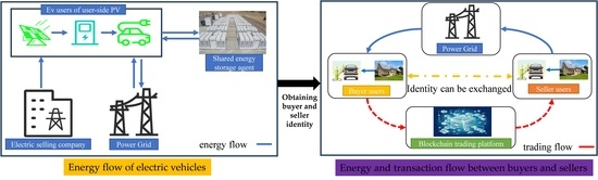
2. Electric Vehicle Electric Energy Trading Architecture
- Obtaining surplus electric energy from electric vehicles: battery status and remaining energy of electric vehicles are monitored through seamless communication between the vehicles and charging facilities;
- Receiving electric energy in energy storage devices: energy storage devices serve as important energy storage units linked to electric vehicle charging facilities in the V2G system. When electric vehicles possess surplus energy, this energy can be transmitted to the energy storage devices through the charging facilities;
- Conversion and storage of electric energy: the remaining electrical energy can be transferred from the electric vehicle to the energy storage device, or from the energy storage device to the electric vehicle.
2.1. Materials and Methods
2.2. Advantages of User-Side PV
3. Multiple Sellers and Buyers Electricity Trading Model
3.1. Charging Behavior of Electric Vehicle Users
3.2. “Multi-Seller–Multi-Buyer” User Division
3.3. “Multi-Seller–Multi-Buyer” Electricity Trading Income Model
4. Blockchain Model of V2G Transactions for EVs
4.1. Blockchain Ledger
4.2. Customer Satisfaction
- , the value of is between and monotonically decreasing;
- , ; therefore, when the difference increases between the buyer’s expected value and the recommended value, the buyer’s satisfaction decreases;
- , where, , ; therefore, when increases, the rate of decline in user satisfaction becomes increasingly faster, that is, the marginal effect decreases.
4.3. Revenue of the Blockchain Platform Operator
5. Revenue of Multiple Operating Entities
5.1. Revenue of State Grid
5.2. Revenue from Electricity Sales Companies
5.3. Share Energy Storage Operator Revenue
6. Solution Method for the Model
7. Example Analysis
7.1. Analysis of “Multi-Seller–Multi-Buyer” Energy Purchase Strategy
7.2. Trading Model Analysis of Multi-Operation Agents Considering “Multi-Seller–Multi-Buyer”
8. Conclusions
- The proposed transaction model incorporates EV buyers and sellers into a transaction system. Simultaneously, blockchain technology is considered a transaction solution for the distributed scenario of EVs, which is more suitable for the development of future scenarios;
- The “multi-seller–multi-buyer” EV surplus electricity trading model presented in this study incorporates regional EVs into the electricity trading framework, efficiently utilizing the surplus electricity of EVs. By allowing EV users to act as sellers, they can achieve corresponding profits. Similarly, buyers can benefit from obtaining electricity at a lower price. The power grid plays an indispensable role in energy transfer. Multiple operating entities, such as electricity sales companies and energy storage operators, also make a profit from this trading process;
- In this model, the user side achieves self-production and self-sales of energy by installing PV systems, significantly reducing reliance on primary energy sources. This approach not only meets the user’s power demand but also delivers the excess energy to users in need and generates profits.
- The model obtains the optimal solution through the improved NGO. Compared to the PSO algorithm and the improved PSO algorithm, the iteration speed of improved NGO is faster and fitness function values are optimal under the same number of iterations.
- A richer EV user model is established, and factors such as EV categories, battery charge and discharge attenuation, and kinetic energy recovery are considered;
- Numerous EVs are aggregated as small energy storage stations and participate in the dispatch and regulation of the power system by the charging and discharging characteristics of the EVs.
- Residual energy trading of EVs is presented in this article. Interchanging surplus energy among EVs to optimize energy utilization can be promoted globally. This makes the consumption of energy can be reduced, and clean energy can be efficiently utilized;
- The security of energy trading is ensured by the application of advanced blockchain technology in EV systems. The decentralized nature of blockchain technology makes the technology easy to roll out in diverse regions worldwide;
- V2G technology has heightened flexibility in the energy market, which enables EV owners to sell their electricity based on energy market prices, secure economic gains, and alleviate price fluctuations in the electricity market;
- A more optimal algorithm can be adopted in utilizing the residual energy of EVs, which gives the technology proposed in this study wider applicability.
Author Contributions
Funding
Data Availability Statement
Acknowledgments
Conflicts of Interest
References
- The Central People’s Government of the People’s Republic of China. China’s Total Automobile Production and Sales Have Ranked First in the World for 14 Consecutive Years [EB/OL]. 2023. Available online: https://www.gov.cn/xinwen/2023-01/12/content_5736536.htm (accessed on 12 January 2023). (In Chinese)
- Yue, H.; Zhang, Q.; Zeng, X.; Huang, W.; Zhang, L.; Wang, J. Optimal Scheduling Strategy of Electric Vehicle Cluster Based on Index Evaluation System. IEEE Trans. Ind. Appl. 2023, 59, 1212–1221. [Google Scholar] [CrossRef]
- Jonas, T.; Daniels, N.; Macht, G. Electric Vehicle User Behavior: An Analysis of Charging Station Utilization in Canada. Energies 2023, 16, 1592. [Google Scholar] [CrossRef]
- Zhang, J.; Yan, J.; Liu, Y.; Zhang, H.; Lv, G. Daily electric vehicle charging load profiles considering demographics of vehicle users. Appl. Energy 2020, 274, 115063. [Google Scholar] [CrossRef]
- Zhang, N.; Zhang, Y.; Ran, L.; Liu, P.; Guo, Y. Robust location and sizing of electric vehicle battery swapping stations considering users’ choice behaviors. J. Energy Storage 2022, 55, 105561. [Google Scholar] [CrossRef]
- Yan, L.; Chen, X.; Zhou, J.; Chen, Y.; Wen, J. Deep Reinforcement Learning for Continuous Electric Vehicles Charging Control with Dynamic User Behaviors. IEEE Trans. Smart Grid 2021, 12, 5124–5134. [Google Scholar] [CrossRef]
- Shchurov, N.I.; Dedov, S.I.; Malozyomov, B.V.; Shtang, A.A.; Martyushev, N.V.; Klyuev, R.V.; Andriashin, S.N. Degradation of Lithium-Ion Batteries in an Electric Transport Complex. Energies 2021, 14, 8072. [Google Scholar] [CrossRef]
- Malozyomov, B.V.; Martyushev, N.V.; Kukartsev, V.A.; Kukartsev, V.V.; Tynchenko, S.V.; Klyuev, R.V.; Zagorodnii, N.A.; Tynchenko, Y.A. Study of Supercapacitors Built in the Start-Up System of the Main Diesel Locomotive. Energies 2023, 16, 3909. [Google Scholar] [CrossRef]
- Bensetti, M.; Kadem, K.; Pei, Y.; Le Bihan, Y.; Labouré, E.; Pichon, L. Parametric Optimization of Ferrite Structure Used for Dynamic Wireless Power Transfer for 3 kW Electric Vehicle. Energies 2023, 16, 5439. [Google Scholar] [CrossRef]
- Qin, H.; Fan, X.; Fan, Y.; Wang, R.; Shang, Q.; Zhang, D. A Computationally Efficient Approach for the State-of-Health Estimation of Lithium-Ion Batteries. Energies 2023, 16, 5414. [Google Scholar] [CrossRef]
- Martin, H.; Buffat, R.; Bucher, D.; Hamper, J.; Raubal, M. Using rooftop photovoltaic generation to cover individual electric vehicle demand—A detailed case study. Renew. Sustain. Energy Rev. 2022, 157, 111969. [Google Scholar] [CrossRef]
- Zheng, B.; Wei, W.; Chen, Y.; Wu, Q.; Mei, S. A peer-to-peer energy trading market embedded with residential shared energy storage units. Appl. Energy 2022, 308, 118400. [Google Scholar] [CrossRef]
- Wang, B.; Xie, M.; Zhang, T.; Wu, M. Sharing Pattern of Distributed Optical Storage System Based on Dynamic Rate Considering Income Equity. Power Syst. Technol. 2021, 45, 2228–2237. [Google Scholar]
- Karakuş, F.; Çiçek, A.; Erdinç, O. Integration of electric vehicle parking lots into railway network considering line losses: A case study of Istanbul M1 metro line. J. Energy Storage 2023, 63, 107101. [Google Scholar] [CrossRef]
- Khan, S.; Sudhakar, K.; Bin Yusof, M.H. Building integrated photovoltaics powered electric vehicle charging with energy storage for residential building: Design, simulation, and assessment. J. Energy Storage 2023, 63, 107050. [Google Scholar] [CrossRef]
- Guo, W.; Yang, P.; Zhang, K.; Wang, C.; Zhuang, W. Power Transaction Method of Microgrid Group Based on Blockchain. High Volt. Eng. 2021, 47, 3810–3818. [Google Scholar]
- Wang, H.; Sun, Y.; Wang, L.; Zhao, P. Frequency Regulation by Virtual Aggregation of Electric Vehicles Based on Consortium Blockchain. Autom. Electr. Power Syst. 2022, 46, 122–131. [Google Scholar]
- Jin, Z.; Wu, R.; Li, G.; Yue, S. Transaction Model for Electric Vehicle Charging Based on Consortium Blockchain. Power Syst. Technol. 2019, 43, 4362–4370. [Google Scholar]
- Sheidaei, F.; Ahmarinejad, A. Multi-stage stochastic framework for energy management of virtual power plants considering electric vehicles and demand response programs. Int. J. Electr. Power Energy Syst. 2020, 120, 106047. [Google Scholar] [CrossRef]
- Brousmiche, K.; Menegazzi, P.; Boudeville, O.; Fantino, E. Peer-to-Peer Energy Market Place Powered by Blockchain and Vehicle-to-Grid Technology. In Proceedings of the 2020 2nd Conference on Blockchain Research & Applications for Innovative Networks and Services (BRAINS), Paris, France, 28–30 September 2020. [Google Scholar]
- Wu, Y.; Wu, Y.; Guerrero, J.M.; Vasquez, J.C. Decentralized transactive energy community in edge grid with positive buildings and interactive electric vehicles. Int. J. Electr. Power Energy Syst. 2022, 135, 107510. [Google Scholar] [CrossRef]
- Pei, F.; Cui, J.; Dong, C.; Wang, H.; Jiang, H.; He, C. The Research Field and Current State-of-art of Blockchain in Distributed Power Trading. Proc. CSEE 2021, 41, 1752–1771. [Google Scholar]
- Zhang, Z.; Lu, L.; Li, Y.; Wang, H.; Ouyang, M. Accurate Remaining Available Energy Estimation of LiFePO4 Battery in Dynamic Frequency Regulation for EVs with Thermal-Electric-Hysteresis Model. Energies 2023, 16, 5239. [Google Scholar] [CrossRef]
- Fachrizal, R.; Shepero, M.; Meer, D.; Munkhammar, J.; Widén, J. Smart charging of electric vehicles considering photovoltaic power production and electricity consumption: A review. eTransportation 2020, 4, 100056. [Google Scholar] [CrossRef]
- Wei, W.; Chen, Y.; Liu, F.; Mei, S.; Tian, F.; Zhang, X. Stackelberg Game Based Retailer Pricing Scheme and EV Charging Management in Smart Residential Area. Power Syst. Technol. 2015, 39, 939–945. [Google Scholar]
- Mumtaz, S.; Al-Dulaimi, A.; Haris, G.; Bo, A. Block Chain and Big Data-Enabled Intelligent Vehicular Communication. IEEE Trans. Intell. Transp. Syst. 2021, 22, 3904–3906. [Google Scholar] [CrossRef]
- Dehghani, M.; Hubálovský, S.; Trojovský, P. Northern Goshawk Optimization: A New Swarm-Based Algorithm for Solving Optimization Problems. IEEE Access 2021, 9, 162059–162080. [Google Scholar] [CrossRef]
- Pradhan, A.; Bisoy, S.; Das, A. A survey on PSO based meta-heuristic scheduling mechanism in cloud computing environment. J. King Saud. Univ. Comput. Inf. Sci. 2022, 34, 4888–4901. [Google Scholar] [CrossRef]


| Time | A | B | C | Time | A | B | C |
|---|---|---|---|---|---|---|---|
| 1 | 0 | 1 | 0 | 13 | 0 | 1 | 1 |
| 2 | 0 | 1 | 0 | 14 | 1 | 0 | 0 |
| 3 | 0 | 1 | 0 | 15 | 0 | 1 | 0 |
| 4 | 0 | 1 | 0 | 16 | 0 | 0 | 1 |
| 5 | 1 | 1 | 0 | 17 | 1 | 0 | 1 |
| 6 | 1 | 0 | 0 | 18 | 1 | 1 | 0 |
| 7 | 1 | 0 | 1 | 19 | 1 | 0 | 1 |
| 8 | 1 | 0 | 1 | 20 | 1 | 0 | 1 |
| 9 | 0 | 0 | 1 | 21 | 1 | 1 | 1 |
| 10 | 0 | 0 | 1 | 22 | 1 | 1 | 1 |
| 11 | 0 | 0 | 1 | 23 | 1 | 1 | 1 |
| 12 | 0 | 1 | 1 | 24 | 1 | 1 | 0 |
| Time | Class A (Yuan) | Class B (Yuan) | Class C (Yuan) | Seller’s Profit (Yuan) |
|---|---|---|---|---|
| 1 | 2.99 | 0 | 1.839 | 4.829 |
| 2 | 0.99 | 0 | 0.15 | 1.14 |
| 3–7 | 0 | 0 | 0 | 0 |
| 8 | 0 | 0.715 | 0 | 0.715 |
| 9 | 0.49 | 64.384 | 0 | 64.874 |
| 10 | 0 | 71.267 | 0 | 71.267 |
| 11 | 4.05 | 14.243 | 0 | 18.293 |
| 12–18 | 0 | 0 | 0 | 0 |
| 19 | 0 | 43.634 | 0 | 43.634 |
| 20 | 0 | 255.975 | 0 | 255.975 |
| 21 | 415.038 | 0 | 0 | 415.038 |
| 22–24 | 0 | 0 | 0 | 0 |
| Time | Class A (Yuan) | Class B (Yuan) | Class C (Yuan) | Seller’s Profit (Yuan) |
|---|---|---|---|---|
| 1 | 1.472 | 0 | 2.676 | 4.148 |
| 2 | 0 | 0 | 1.296 | 1.296 |
| 3–7 | 0 | 0 | 0 | 0 |
| 8 | 0 | 0.853 | 0 | 0.853 |
| 9 | 0 | 53.383 | 0 | 53.383 |
| 10 | 0 | 68.745 | 0 | 68.745 |
| 11 | 0 | 36.657 | 0 | 36.657 |
| 12–19 | 0 | 0 | 0 | 0 |
| 20 | 0 | 207.644 | 0 | 207.644 |
| 21 | 231.498 | 0 | 0 | 231.498 |
| 22–24 | 0 | 0 | 0 | 0 |
| Time | Class A (Yuan) | Class B (Yuan) | Class C (Yuan) | Seller’s Profit (Yuan) |
|---|---|---|---|---|
| 1 | 1.993 | 0 | 3.231 | 5.224 |
| 2 | 0 | 0 | 0.767 | 0.767 |
| 3–7 | 0 | 0 | 0 | 0 |
| 8 | 0 | 0.677 | 0 | 0.677 |
| 9 | 0 | 42.82 | 0 | 42.82 |
| 10 | 0 | 140.505 | 0 | 140.505 |
| 11 | 0 | 36.655 | 0 | 36.655 |
| 12–19 | 0 | 0 | 0 | 0 |
| 20 | 0 | 125.583 | 0 | 125.583 |
| 21 | 308.668 | 0 | 0 | 308.668 |
| 22–24 | 0 | 0 | 0 | 0 |
| User Transactions | No Blockchain Is Used | Using Blockchain |
|---|---|---|
| Credibility | Third-party credit guarantee | Open, transparent, and trusted |
| Means of information interaction | Traditional centralized transaction model | Blockchain ledger |
| Average cost of electricity | 1.3 (Yuan/kW·h) | 0.74 (Yuan/kW·h) |
| Utilization of new energy | Low | High |
| Parameter | Improved NGO | Improved PSO | PSO |
|---|---|---|---|
| Iterations (times) | 500 | 500 | 500 |
| Run time (seconds) | 1.764 | 1.868 | 3.583 |
| Revenue situation (Yuan) | 2922.221 | 2883.968 | 2621.941 |
Disclaimer/Publisher’s Note: The statements, opinions and data contained in all publications are solely those of the individual author(s) and contributor(s) and not of MDPI and/or the editor(s). MDPI and/or the editor(s) disclaim responsibility for any injury to people or property resulting from any ideas, methods, instructions or products referred to in the content. |
© 2023 by the authors. Licensee MDPI, Basel, Switzerland. This article is an open access article distributed under the terms and conditions of the Creative Commons Attribution (CC BY) license (https://creativecommons.org/licenses/by/4.0/).
Share and Cite
Wang, X.; Wei, J.; Wen, F.; Wang, K. A Trading Mode Based on the Management of Residual Electric Energy in Electric Vehicles. Energies 2023, 16, 6317. https://doi.org/10.3390/en16176317
Wang X, Wei J, Wen F, Wang K. A Trading Mode Based on the Management of Residual Electric Energy in Electric Vehicles. Energies. 2023; 16(17):6317. https://doi.org/10.3390/en16176317
Chicago/Turabian StyleWang, Xiuli, Junkai Wei, Fushuan Wen, and Kai Wang. 2023. "A Trading Mode Based on the Management of Residual Electric Energy in Electric Vehicles" Energies 16, no. 17: 6317. https://doi.org/10.3390/en16176317
APA StyleWang, X., Wei, J., Wen, F., & Wang, K. (2023). A Trading Mode Based on the Management of Residual Electric Energy in Electric Vehicles. Energies, 16(17), 6317. https://doi.org/10.3390/en16176317