


Time Series Forecasting for Energy Production in Stand-Alone and Tracking Photovoltaic Systems Based on Historical Measurement Data


Abstract
:1. Introduction
- Neural-network-based energy yield models were developed and compared with other prediction models for two types of installed photovoltaic panels: a fixed system and a solar tracker. These systems were located in a humid continental climate.
- A large dataset was used for the training and test processes. It was shown that tuning the network’s hyperparameters had a significant impact on the forecast accuracy and computational time.
- To assess the prediction performance of the regression algorithms (used with continuous data) and the classification algorithms (used with discrete data), quantitative metrics were adopted.
- It was shown that it is not advisable to rely on one metric (R-squared) as a universal indicator of forecast quality.
- This article focuses on forecasting electricity production in small photovoltaic systems. Consequently, an analysis of the climate variables that affect the forecasting of electricity production was also carried out, taking into account the availability of information in historical measurement data.
2. Literature Review
3. Materials and Methods
- Forecasts were made for a fixed-tilt system and a solar-tracking system due to the identical technical parameters of both PV plants;
- Forecasts were intended to specify day-ahead energy production expressed in kWh;
- Forecasts were made on the basis of the daily maximum and minimum temperatures, atmospheric pressure, wind speed, and an integer timestamp (a day of the year).
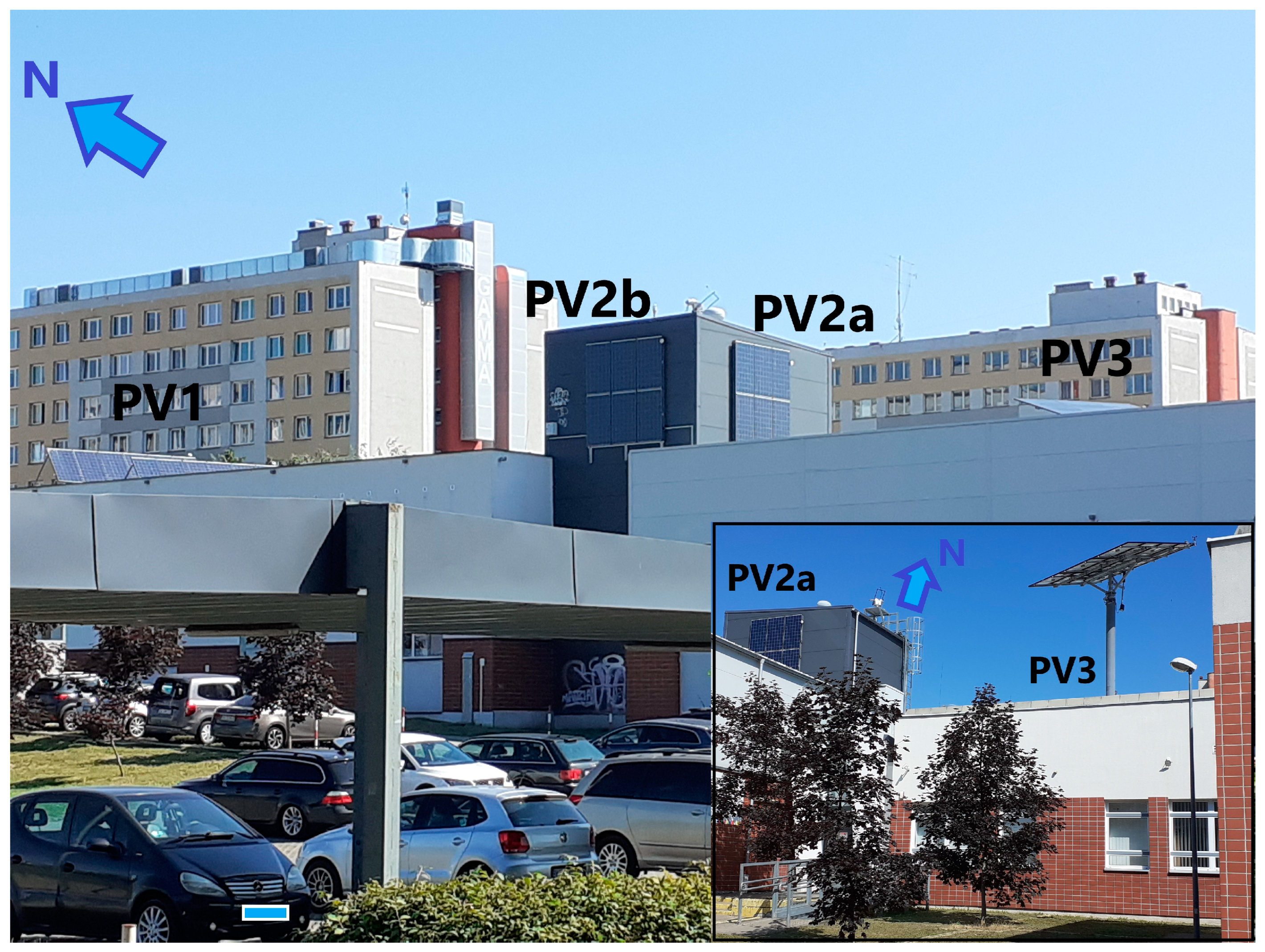
- A fixed-tilt system with panels in the optimal direction, with a nominal power of 3.0 kWp (PV1);
- A solar-tracking system, with a nominal power of 3.0 kWp (PV3);
- A fixed-tilt system with panels that face the south-east, with a nominal power of 1.5 kWp (PV2a);
- A fixed-tilt system with panels that face the south-west, with a nominal power of 1.5 kWp (PV2b).
- The date converted to a day number from the analyzed period (timestamp);
- The energy produced by the PV1 unit (energy pv1);
- The energy produced by the PV1 unit- classified (energy pv1-class);
- The energy produced by the PV3 unit (energy pv3);
- The energy produced by the PV3 unit- classified (energy pv3-class);
- The maximal temperature (temp-max);
- The minimal temperature (temp-min);
- The atmospheric pressure (pressure);
- The average wind speed (wind-speed).
4. Model Performance Metrics and Statistical Tests
- MAE (mean absolute error);
- MSE (mean squared error);
- RMSE (root mean squared error);
- The coefficient of determination, R2.
5. Results and Discussion
5.1. Feature Selection
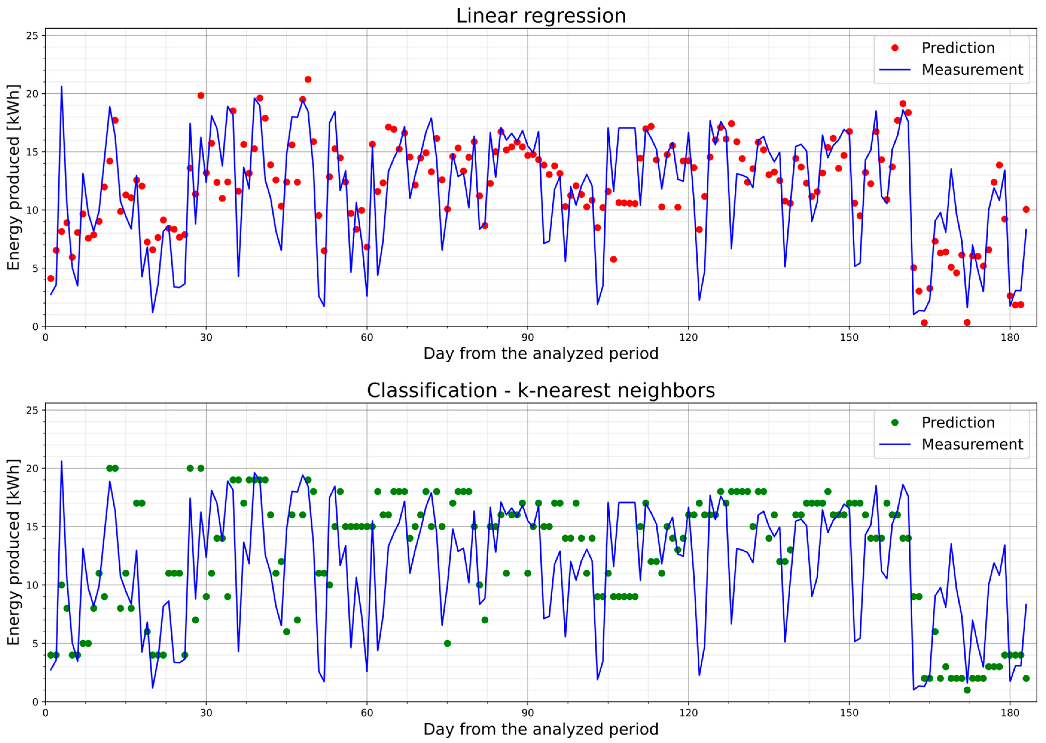
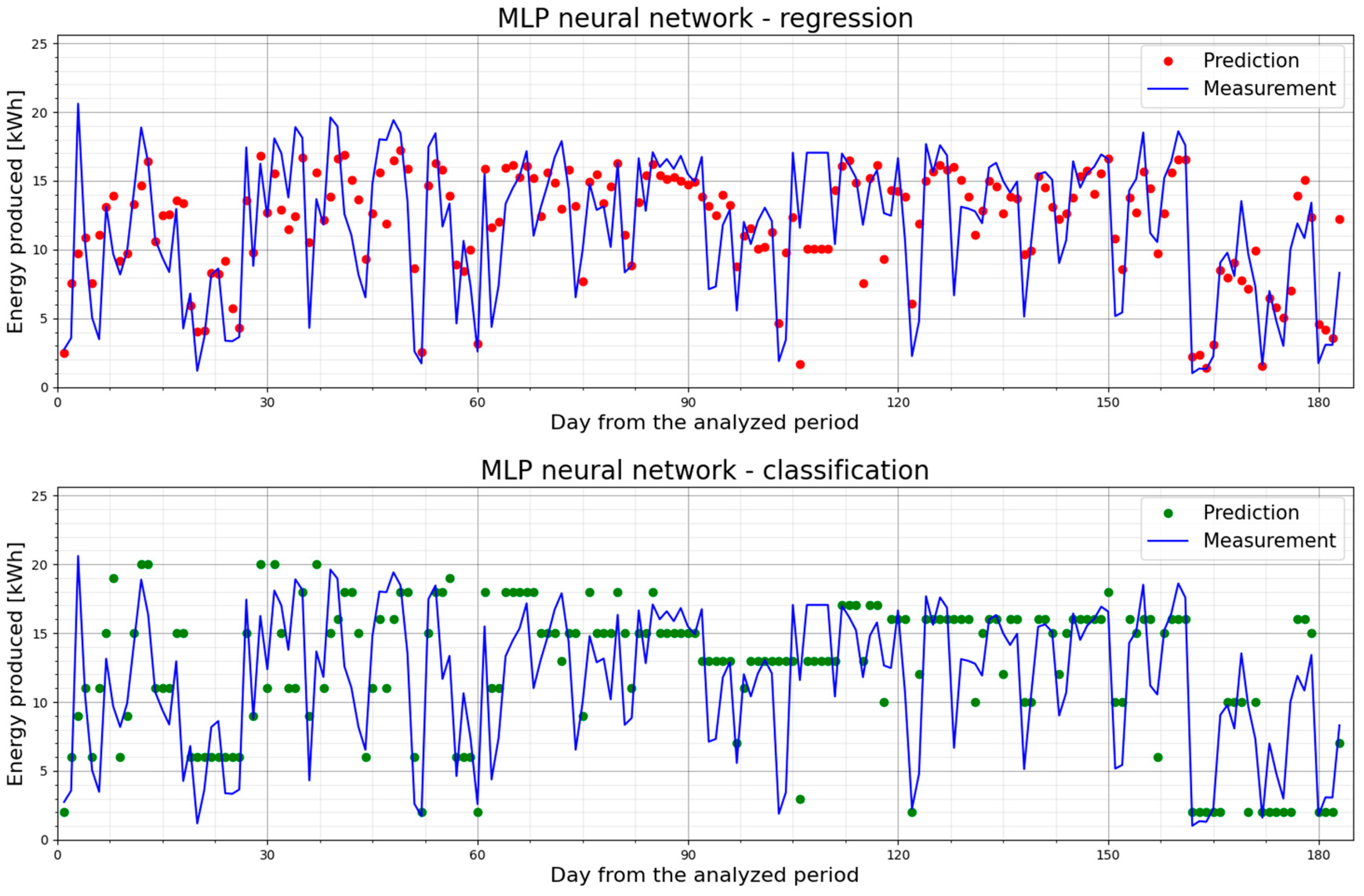
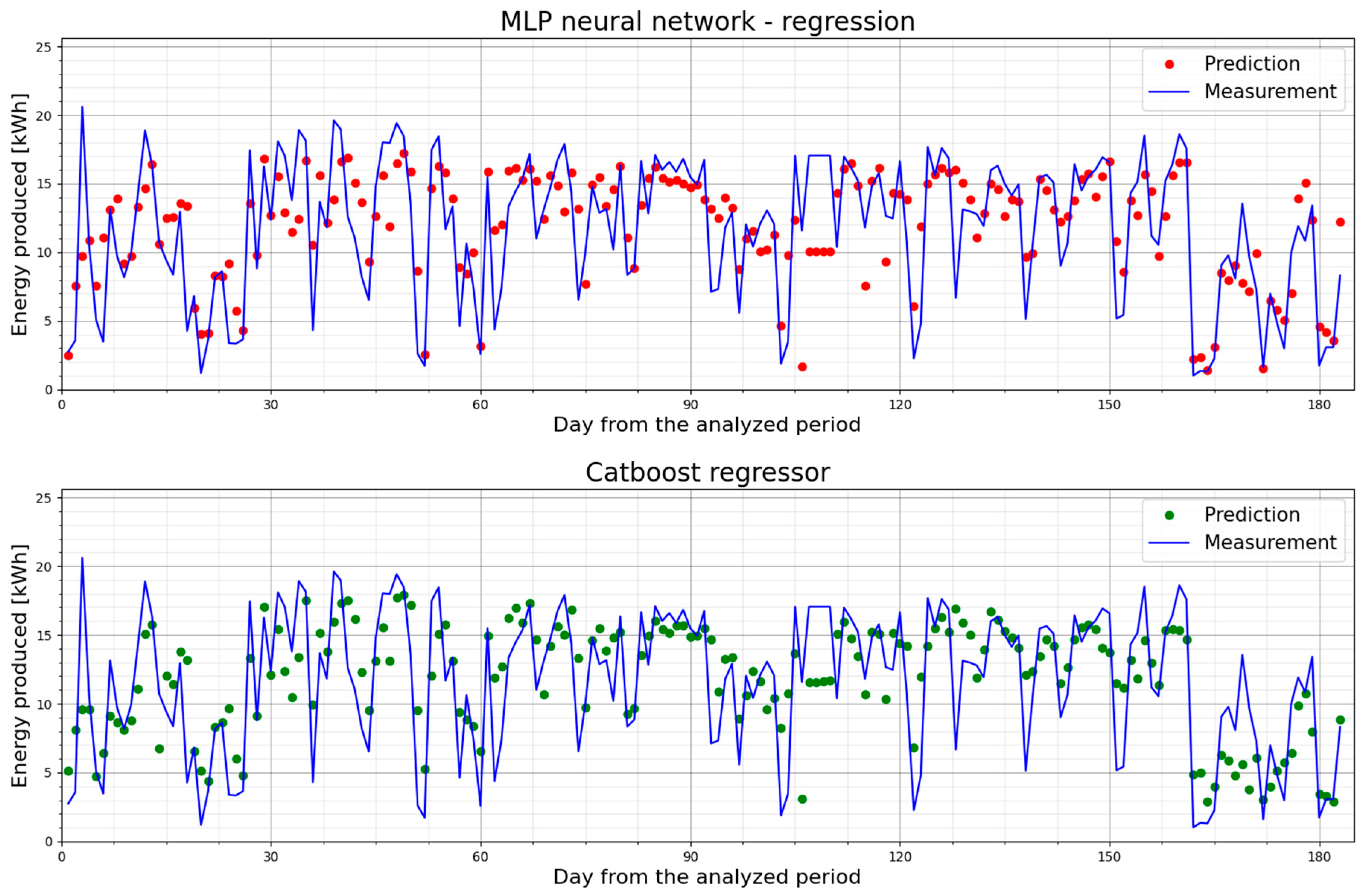
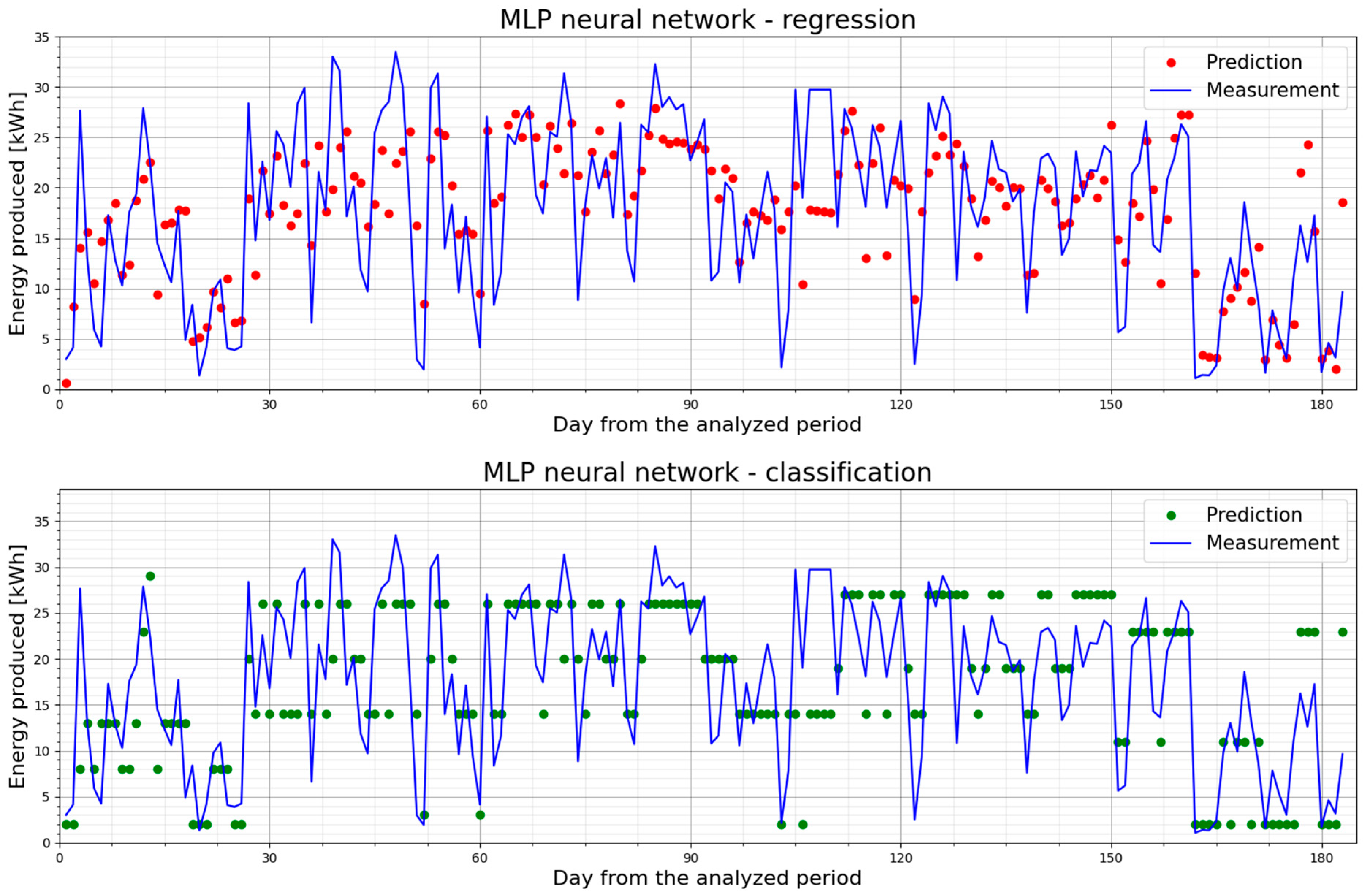
5.2. PV1—Prediction Models and Their Performance
5.3. PV3—Prediction Models and Their Performance
5.4. PV1 vs. PV3—A Comparison of Quantitative Metrics
5.5. DM Test to Distinguish the Significant Differences in the Forecasting Accuracy
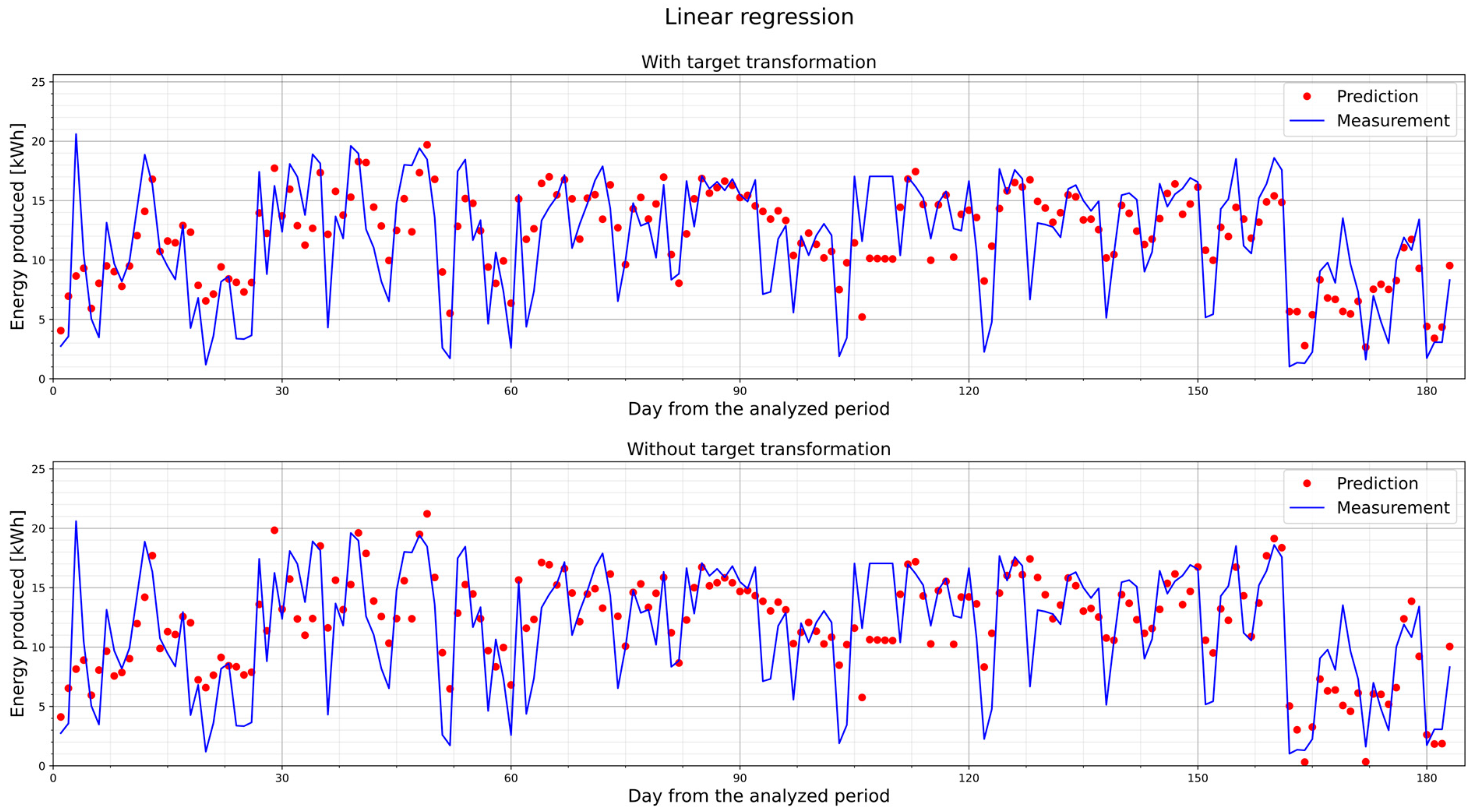
5.6. Improving Regression Model Performance Using a Target Transformation
- Function transformation—logarithmic, log(1 + x), and exponential, exp(x) – 1, functions were used to transform the targets before training a linear regression model and using it for prediction (Table 14);
- Feature scaling data—each feature was scaled to a 0–1 range (MinMaxScaler), and inverse transformation was used (Table 15).
5.7. The Performance of the Selected Models after Splitting the Dataset
6. Conclusions
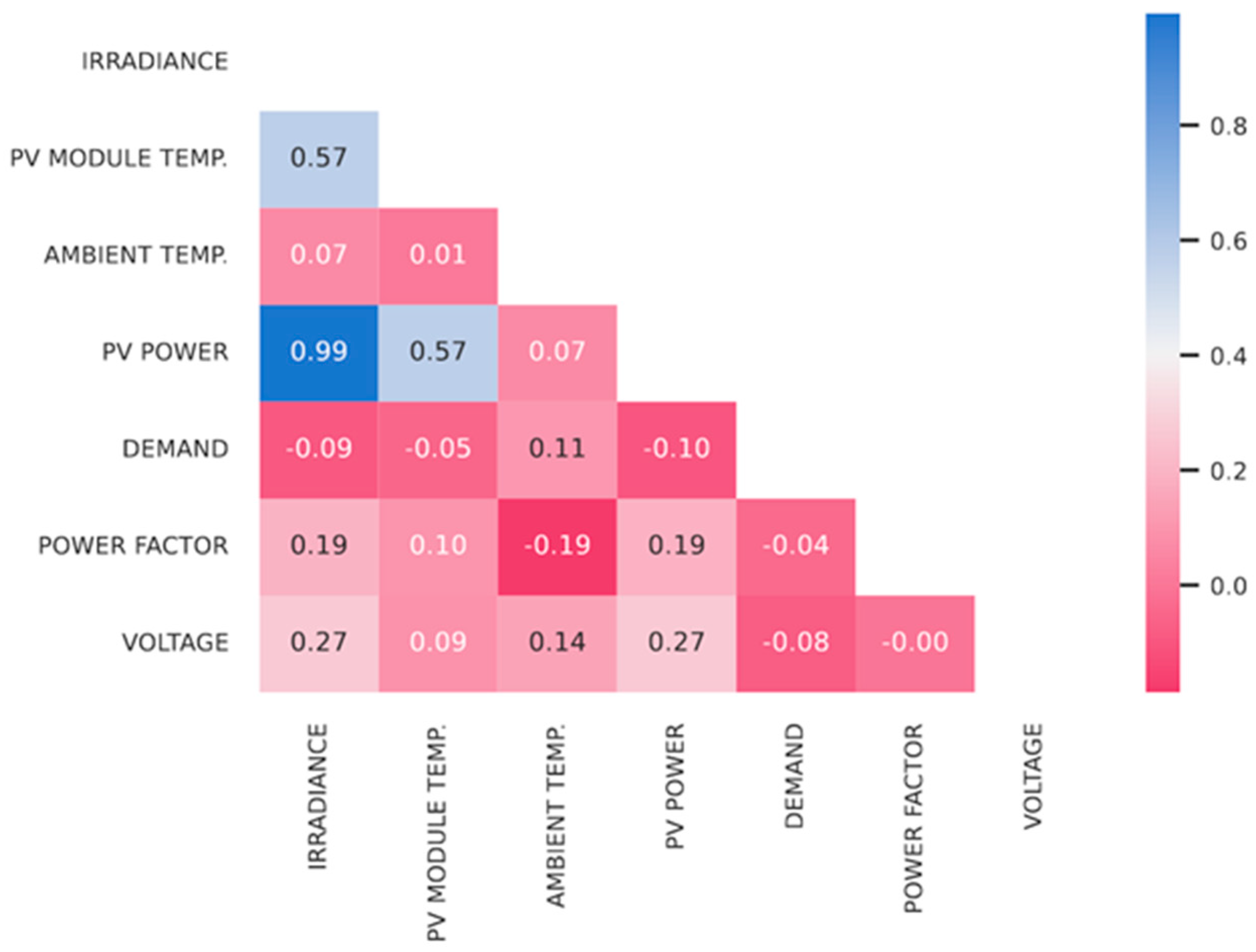
- The number of input variables utilized in the modeling can affect the forecasting performance. As evident from Table 5, the strongest intercorrelation existed between the minimum and maximum temperatures. The minimum and maximum temperatures had a considerable periodicity (intercorrelations with the timestamp). However, the absence of a minimum temperature in the MLPRegressor model had a negative impact on the forecasts, with a decrease in the value of the R-squared coefficient from 0.6 to about 0.4.
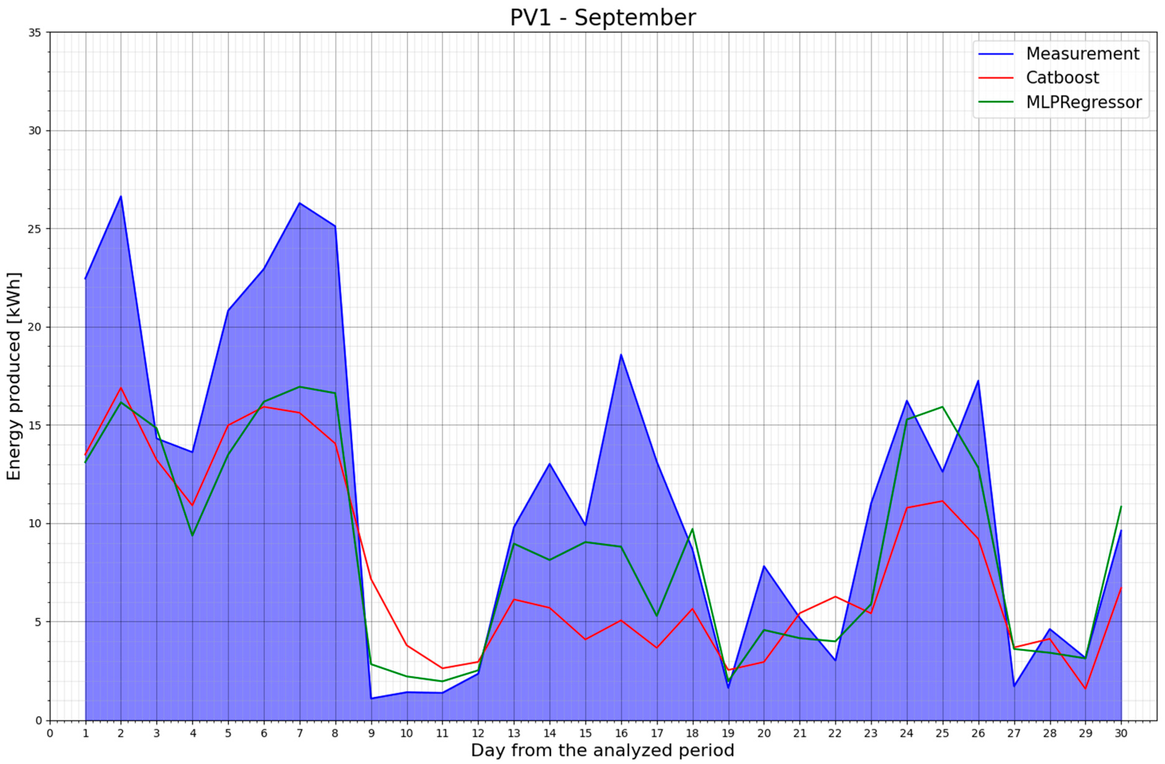
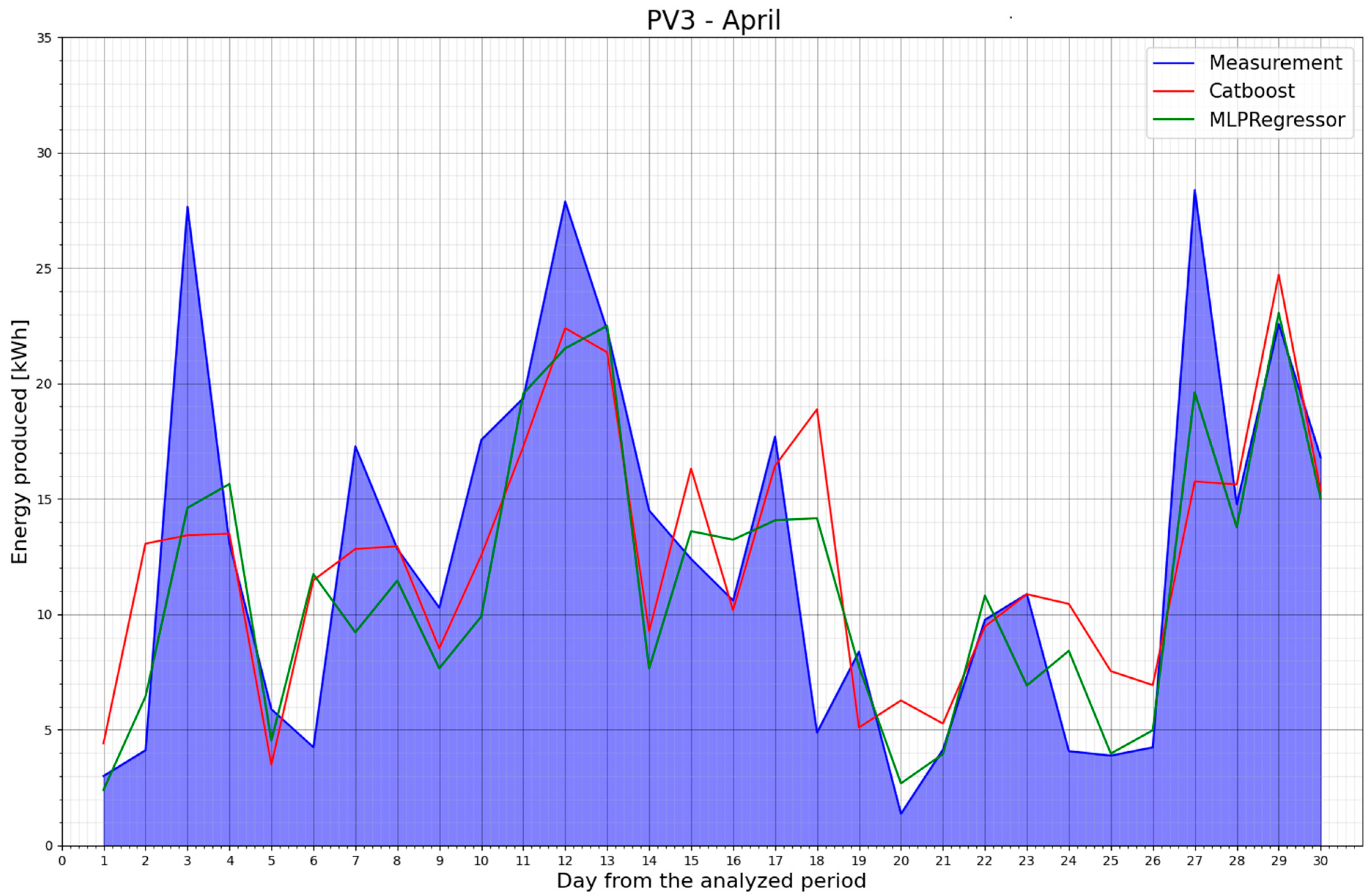
- Splitting the dataset can boost the metric values. Table 16 presents a comparison between the MLPRegressor and CatBoostRegressor models after splitting the dataset. The MLPRegressor model proved to be more effective for forecasting within individual data groups (monthly data). The MLPRegressor model yielded the highest R-squared value for September 2022, exceeding 0.8. This could mean that this month had the most repeated weather conditions in Poland compared to the months of September in the previous seven years.
- To enhance the model performance, the periodicity of light could be taken into consideration. Also, seasonality (weekly or monthly repeating patterns) could be detected and incorporated in the forecasting.
Author Contributions
Funding
Data Availability Statement
Acknowledgments
Conflicts of Interest
References
- Vita, V.; Fotis, G.; Pavlatos, C.; Mladenov, V. A New Restoration Strategy in Microgrids after a Blackout with Priority in Critical Loads. Sustainability 2023, 15, 1974. [Google Scholar] [CrossRef]
- Soto, E.A.; Bosman, L.B.; Wollega, E.; Leon-Salas, W.D. Analysis of Grid Disturbances Caused by Massive Integration of Utility Level Solar Power Systems. Eng 2022, 3, 236–253. [Google Scholar] [CrossRef]
- Paska, J.; Surma, T.; Terlikowski, P.; Zagrajek, K. Electricity Generation from Renewable Energy Sources in Poland as a Part of Commitment to the Polish and EU Energy Policy. Energies 2020, 13, 4261. [Google Scholar] [CrossRef]
- Alaraj, M.; Kumar, A.; Alsaidan, I.; Rizwan, M.; Jamil, M. Energy Production Forecasting from Solar Photovoltaic Plants Based on Meteorological Parameters for Qassim Region, Saudi Arabia. IEEE Access 2021, 9, 83241–83251. [Google Scholar] [CrossRef]
- ElNozahy, M.S.; Salama, M.M.A. Technical impacts of grid-connected photovoltaic systems on electrical networks-a review. J. Renew. Sustain. Energy 2013, 5, 032702. [Google Scholar] [CrossRef]
- Yin, L.; Cao, X.; Liu, D. Weighted fully-connected regression networks for one-day-ahead hourly photovoltaic power forecasting. Appl. Energy 2023, 332, 120527. [Google Scholar] [CrossRef]
- Ulbricht, R.; Fischer, U.; Lehner, W.; Donker, H. First steps towards a systematical optimized strategy for solar energy supply forecasting. In Proceedings of the European Conference on Machine Learning and Principles and Practice of Knowledge Discovery in Databases (ECMLPKDD 2013), Prague, Czech Republic, 23–27 September 2013. [Google Scholar]
- Ssekulima, E.B.; Anwar, M.B.; Al Hinai, A.; El Moursi, M.S. Wind speed and solar irradiance forecasting techniques for enhanced renewable energy integration with the grid: A review. IET Renew. Power Gener. 2016, 10, 885–898. [Google Scholar] [CrossRef]
- Fara, L.; Diaconu, A.; Craciunescu, D.; Fara, S. Forecasting of energy production for photovoltaic systems based on ARIMA and ANN advanced models. Int. J. Photoenergy 2021, 2021, 6777488. [Google Scholar] [CrossRef]
- Lezmi, E.; Xu, J. Time Series Forecasting with Transformer Models and Application to Asset Management; SSRN: Rochester, NY, USA, 2023. [Google Scholar] [CrossRef]
- Yang, Y.; Lu, J. A Fusion Transformer for Multivariable Time Series Forecasting: The Mooney Viscosity Prediction Case. Entropy 2022, 24, 528. [Google Scholar] [CrossRef]
- Petropoulos, F.; Apiletti, D.; Assimakopoulos, V.; Babai, M.Z.; Barrow, D.K.; Ben Taieb, S.; Bergmeir, C.; Bessa, R.J.; Bijak, J.; Boylan, J.E.; et al. Forecasting: Theory and practice. Int. J. Forecast. 2022, 38, 705–871. [Google Scholar] [CrossRef]
- Mohamad Radzi, P.N.L.; Akhter, M.N.; Mekhilef, S.; Mohamed Shah, N. Review on the Application of Photovoltaic Forecasting Using Machine Learning for Very Short- to Long-Term Forecasting. Sustainability 2023, 15, 2942. [Google Scholar] [CrossRef]
- Raschka, S.; Patterson, J.; Nolet, C. Machine Learning in Python: Main Developments and Technology Trends in Data Science, Machine Learning, and Artificial Intelligence. Information 2020, 11, 193. [Google Scholar] [CrossRef]
- Petropoulos, F.; Makridakis, S.; Assimakopoulos, V.; Nikolopoulos, K. ‘Horses for Courses’ in demand forecasting. Eur. J. Oper. Res. 2014, 237, 152–163. [Google Scholar] [CrossRef]
- Li, G.; Wei, X.; Yang, H. Decomposition integration and error correction method for photovoltaic power forecasting. Measurement 2023, 208, 112462. [Google Scholar] [CrossRef]
- Sarmas, E.; Strompolas, S.; Marinakis, V.; Santori, F.; Bucarelli, M.A.; Doukas, H. An Incremental Learning Framework for Photovoltaic Production and Load Forecasting in Energy Microgrids. Electronics 2022, 11, 3962. [Google Scholar] [CrossRef]
- Colak, M.; Yesilbudak, M.; Bayindir, R. Daily Photovoltaic Power Prediction Enhanced by Hybrid GWO-MLP, ALO-MLP and WOA-MLP Models Using Meteorological Information. Energies 2020, 13, 901. [Google Scholar] [CrossRef]
- Khademi, M.; Moadel, M.; Khosravi, A. Power Prediction and Technoeconomic Analysis of a Solar PV Power Plant by MLP-ABC and COMFAR III, considering Cloudy Weather Conditions. Int. J. Chem. Eng. 2016, 2016, 1031943. [Google Scholar] [CrossRef]
- Abdel-Nasser, M.; Mahmoud, K. Accurate photovoltaic power forecasting models using deep LSTM-RNN. Neural Comput. Appl. 2019, 31, 2727–2740. [Google Scholar] [CrossRef]
- Sala, S.; Amendola, A.; Leva, S.; Mussetta, M.; Niccolai, A.; Ogliari, E. Comparison of Data-Driven Techniques for Nowcasting Applied to an Industrial-Scale Photovoltaic Plant. Energies 2019, 12, 4520. [Google Scholar] [CrossRef]
- Wang, H.; Yi, H.; Peng, J.; Wang, G.; Liu, Y.; Jiang, H.; Liu, W. Deterministic and probabilistic forecasting of photovoltaic power based on deep convolutional neural network. Energy Convers. Manag. 2017, 153, 409–422. [Google Scholar] [CrossRef]
- Zhu, T.; Guo, Y.; Li, Z.; Wang, C. Solar Radiation Prediction Based on Convolution Neural Network and Long Short-Term Memory. Energies 2021, 14, 8498. [Google Scholar] [CrossRef]
- Trabelsi, M.; Massaoudi, M.; Chihi, I.; Sidhom, L.; Refaat, S.S.; Huang, T.; Oueslati, F.S. An Effective Hybrid Symbolic Regression–Deep Multilayer Perceptron Technique for PV Power Forecasting. Energies 2022, 15, 9008. [Google Scholar] [CrossRef]
- Cabezón, L.; Ruiz, L.G.B.; Criado-Ramón, D.; Gago, E.J.; Pegalajar, M.C. Photovoltaic Energy Production Forecasting through Machine Learning Methods: A Scottish Solar Farm Case Study. Energies 2022, 15, 8732. [Google Scholar] [CrossRef]
- Wang, Z.; Koprinska, I.; Rana, M. Clustering based methods for solarpower forecasting. In Proceedings of the 2016 International Joint Conference on Neural Networks (IJCNN), Vancouver, BC, Canada, 24–29 July 2016; pp. 1487–1494. [Google Scholar] [CrossRef]
- Klyuev, R.V.; Morgoev, I.D.; Morgoeva, A.D.; Gavrina, O.A.; Martyushev, N.V.; Efremenkov, E.A.; Mengxu, Q. Methods of Forecasting Electric Energy Consumption: A Literature Review. Energies 2022, 15, 8919. [Google Scholar] [CrossRef]
- Sunthornnapha, T. Utilization of MLP and Linear Regression Methods to Build a Reliable Energy Baseline for Self-benchmarking Evaluation. Energy Procedia 2017, 141, 189–193. [Google Scholar] [CrossRef]
- Purlu, M.; Turkay, B.E. Estimating the Distributed Generation Unit Sizing and Its Effects on the Distribution System by Using Machine Learning Methods. Elektron. Elektrotech. 2021, 27, 24–32. [Google Scholar] [CrossRef]
- Dellino, G.; Laudadio, T.; Mari, R.; Mastronardi, N.; Meloni, C.; Vergura, S. Energy production forecasting in a PV plant using transfer function models. In Proceedings of the 2015 IEEE 15th International Conference on Environment and Electrical Engineering (EEEIC), Rome, Italy, 10–13 June 2015; pp. 1379–1383. [Google Scholar] [CrossRef]
- Khilar, R.; Suba, G.M.; Kumar, T.S.; Samson Isaac, J.; Shinde, S.K.; Ramya, S.; Prabhu, V.; Erko, K.G. Improving the Efficiency of Photovoltaic Panels Using Machine Learning Approach. Int. J. Photoenergy 2022, 2022, 4921153. [Google Scholar] [CrossRef]
- Olabi, A.G.; Abdelkareem, M.A.; Semeraro, C.; Radi, M.A.; Rezk, H.; Muhaisen, O.; Al-Isawi, O.A.; Sayed, E.T. Artificial neural networks applications in partially shaded PV systems. Therm. Sci. Eng. Prog. 2023, 37, 101612. [Google Scholar] [CrossRef]
- Bhatnagar, P.; Nema, R.K. Maximum power point tracking control techniques: State-of-the-art in photovoltaic applications. Renew. Sustain. Energy Rev. 2013, 23, 224–241. [Google Scholar] [CrossRef]
- Kermadi, M.; Berkouk, E.M. Artificial intelligence-based maximum power point tracking controllers for Photovoltaic systems: Comparative study. Renew. Sustain. Energy Rev. 2017, 69, 369–386. [Google Scholar] [CrossRef]
- Andrade, C.H.T.d.; Melo, G.C.G.d.; Vieira, T.F.; Araújo, Í.B.Q.d.; Medeiros Martins, A.d.; Torres, I.C.; Brito, D.B.; Santos, A.K.X. How Does Neural Network Model Capacity Affect Photovoltaic Power Prediction? A Study Case. Sensors 2023, 23, 1357. [Google Scholar] [CrossRef] [PubMed]
- Das, U.K.; Tey, K.S.; Seyedmahmoudian, M.; Mekhilef, S.; Idris, M.Y.I.; Van Deventer, W.; Horan, B.; Stojcevski, A. Forecasting of photovoltaic power generation and model optimization: A review. Renew. Sustain. Energy Rev. 2018, 81, 912–928. [Google Scholar] [CrossRef]
- Zhong, J.; Liu, L.; Sun, Q.; Wang, X. Prediction of Photovoltaic Power Generation Based on General Regression and Back Propagation Neural Network. Energy Procedia 2018, 152, 1224–1229. [Google Scholar] [CrossRef]
- Icel, Y.; Mamis, M.S.; Bugutekin, A.; Gursoy, M.I. Photovoltaic Panel Efficiency Estimation with Artificial Neural Networks: Samples of Adiyaman, Malatya and Sanliurfa. Int. J. Photoenergy 2019, 2019, 6289021. [Google Scholar] [CrossRef]
- Son, J.; Park, Y.; Lee, J.; Kim, H. Sensorless PV Power Forecasting in Grid-Connected Buildings through Deep Learning. Sensors 2018, 18, 2529. [Google Scholar] [CrossRef]
- Eseye, A.T.; Zhang, J.; Zheng, D. Short-term photovoltaic solar power forecasting using a hybrid Wavelet-PSO-SVM model based on SCADA and Meteorological information. Renew. Energy 2018, 118, 357–367. [Google Scholar] [CrossRef]
- Paterova, T.; Prauzek, M. Estimating Harvestable Solar Energy from Atmospheric Pressure Using Deep Learning. Elektron. Elektrotech. 2021, 27, 18–25. [Google Scholar] [CrossRef]
- Kusznier, J.; Wojtkowski, W. Impact of climatic conditions on PV panels operation in a photovoltaic power plant. In Proceedings of the 2019 15th Selected Issues of Electrical Engineering and Electronics (WZEE), Zakopane, Poland, 8–10 December 2019. [Google Scholar] [CrossRef]
- Munir, M.A.; Khattak, A.; Imran, K.; Ulasyar, A.; Khan, A. Solar PV Generation Forecast Model Based on the Most Effective Weather Parameters. In Proceedings of the 2019 International Conference on Electrical, Communication, and Computer Engineering (ICECCE), Swat, Pakistan, 24–25 July 2019. [Google Scholar] [CrossRef]
- WS501-UMB Smart Weather Sensor. Available online: https://www.lufft.com/products/compact-weather-sensors-293/ws501-umb-smart-weather-sensor-1839/ (accessed on 1 February 2023).
- Machine Learning in Python. Available online: https://scikit-learn.org/stable/index.html (accessed on 1 February 2023).
- Geron, A. Hands-On Machine Learning with Scikit-Learn, Keras, and TensorFlow, Concepts, Tools, and Techniques to Build Intelligent Systems; O’Reilly Media Inc.: Sevastopo, CA, USA, 2019. [Google Scholar]
- Albon, C. Machine Learning with Python Cookbook, Practical Solutions from Preprocessing to Deep Learning; O’Reilly Media Inc.: Sevastopo, CA, USA, 2018. [Google Scholar]
- Murtagh, F. Multilayer perceptrons for classification and regression. Neurocomputing 1991, 2, 183–197. [Google Scholar] [CrossRef]
- Xiang, W.; Xu, P.; Fang, J.; Zhao, Q.; Gu, Z.; Zhang, Q. Multi-dimensional data-based medium- and long-term power-load forecasting using double-layer CatBoost. Energy Rep. 2022, 8, 8511–8522. [Google Scholar] [CrossRef]
- Diebold, F.X.; Mariano, R.S. Comparing predictive accuracy. J. Bus. Econ. Stat. 1995, 13, 253–264. [Google Scholar]
- Harvey, D.; Leybourne, S.; Newbold, P. Testing the equality of prediction mean squared errors. Int. J. Forecast. 1997, 13, 281–291. [Google Scholar] [CrossRef]
- Huber, P.J. Robust Estimation of a Location Parameter. Ann. Math. Stat. 1964, 35, 73–101. [Google Scholar] [CrossRef]
- Kharlova, E.; May, D.; Musilek, P. Forecasting Photovoltaic Power Production using a Deep Learning Sequence to Sequence Model with Attention. In Proceedings of the 2020 International Joint Conference on Neural Networks (IJCNN), Glasgow, UK, 17–24 July 2020; pp. 1–7. [Google Scholar] [CrossRef]
- Yang, G. Asymptotic tracking with novel integral robust schemes for mismatched uncertain nonlinear systems. Int. J. Robust Nonlinear Control 2023, 33, 1988–2002. [Google Scholar] [CrossRef]
- Khan, Z.A.; Hussain, T.; Baik, S.W. Dual stream network with attention mechanism for photovoltaic power forecasting. Appl. Energy 2023, 338, 120916. [Google Scholar] [CrossRef]


| Inputs | R-Squared Coefficient |
|---|---|
| Irradiance on module | 0.998 |
| Module temperature | 0.587 |
| Wind speed | 0.447 |
| Relative humidity | −0.362 |
| Publication | Model | R2 | Comments | Features | PV Power, Location | Datasets |
|---|---|---|---|---|---|---|
| [19] | MLP ABC | 0.95 | Separate forecasting for cloudy and sunny conditions | Total power, total irradiance, ambient temperature, and humidity | 3.2 kWp, Tehran, Iran, elevation 1548 m | 6895 of sunny, 3090 of cloudy, 680 for testing |
| MLP ABC | 0.83 | Forecasting under all conditions | ||||
| [21] | LR | 0.78 | Forecast 8 h ahead | Deterministic and stochastic power, stochastic irradiance, ambient temperature, and panel temperature | 1 MWp, Eni Energy Company, Italy | 103,740 samples, 80% for training, 20% for testing |
| MLP | 0.69 | Forecast 8 h ahead | ||||
| KNN | 0.35 | Forecast 8 h ahead | ||||
| [25] | KNN | 0.88 | Forecast 1 h ahead | Year, month, day, hour, present energy, and energy 1, 2, and 3 h(s) ago | 50 kWp, Cononsyth, Scotland | 54,000 samples |
| MLP | 0.87 | Forecast 1 h ahead | ||||
| LSTM | 0.85 | Forecast 1 h ahead | ||||
| [39] | DNN | 0.93 | Forecast 1 d ahead | Weather forecast data from the Korean Meteorological Administration | 2.448 kWp, Seoul, South Korea, rooftop PV system | 3798 entries, 3000 for training, 798 for testing |
| Measured Quantity | Method | Measurement Performance |
|---|---|---|
| Speed and wind direction | Ultrasonic | Wind direction |
| Range: 0–359.9° Accuracy: RMSE < 3° at speed > 1 m/s | ||
| Wind speed | ||
| Range: 0–75 m/s Accuracy: ±0.3 m/s or ±3% (0–35 m/s) ±5% (>35 m/s) RMS | ||
| Air temperature | NTC | Range: from −50 °C to +60 °C Accuracy: ±0.2 °C (−20–+50 °C), ±0.5 °C (>−30 °C) |
| Relative humidity | Capacitive | Range: 0–100% RH Accuracy: ±2% RH |
| Atmospheric pressure | MEMS | Range: 300–1200 hPa Accuracy: ±0.5 hPa (0–+40 °C) |
| Irradiance | Pyranometer | Range: 2000 W/m² (300–2800 nm) |
| Timestamp | Energy PV1 | Energy PV1 Class | Energy PV3 | Energy PV3 Class | Temp Max | Temp Min | Pressure | Wind Speed |
|---|---|---|---|---|---|---|---|---|
| Day No. | kWh | kWh | kWh | kWh | °C | °C | hPa | m/s |
| 1 | 4.534 | 5 | 3.772 | 4 | 5.7 | 1.9 | 978.3 | 5.7 |
| 2 | 4.087 | 4 | 3.376 | 3 | 5.5 | −0.7 | 984.2 | 3.7 |
| 3 | 5.009 | 5 | 4.326 | 4 | 6.5 | −1.1 | 989.2 | 2.9 |
| Power Plant PV1 (PV3) | ||||||
|---|---|---|---|---|---|---|
| energy | temp max | temp min | pressure | wind speed | timestamp | |
| energy | 1 | - | - | - | - | - |
| temp max | 0.40 (0.45) | 1 | - | - | - | - |
| temp min | 0.06 (0.14) | 0.83 | 1 | - | - | - |
| pressure | 0.32 (0.29) | 0.06 | −0.09 | 1 | - | - |
| wind speed | −0.08 (−0.07) | −0.12 | −0.10 | −0.07 | 1 | - |
| timestamp | −0.11 (−0.13) | 0.36 | 0.47 | 0.12 | −0.08 | 1 |
| Model | MAE [kWh] | MAE [%] | MSE [kWh2] | RMSE [kWh] | R2 | |
|---|---|---|---|---|---|---|
| Linear regression 1 | 2.65 | 42.05 | 11.96 | 3.46 | 0.544 | |
| ARIMA | 3.79 | 75.21 | 22.25 | 4.72 | 0.152 | |
| KNN 2 | 4.07 | 59.96 | 25.88 | 5.09 | 0.014 | |
| XGBRegressor | 2.90 | 53.08 | 13.19 | 3.63 | 0.497 | |
| RandomForestRegressor | 2.85 | 48.32 | 13.11 | 3.62 | 0.500 | |
| CatBoostRegressor 5 | 2.64 | 41.38 | 11.79 | 3.43 | 0.551 | |
| MLP | Regressor 3 | 2.43 | 37.48 | 3.22 | 1.79 | 0.605 |
| Classifier 4 | 2.87 | 34.94 | 3.80 | 1.95 | 0.450 | |
| Energy PV1 Class with a Width of 0.5 kWh | Energy PV1 Class with a Width of 1 kWh | |||||
|---|---|---|---|---|---|---|
| Number of Neighbors k | RMSE [kWh] | R2 | Computation Time [s] | RMSE [kWh] | R2 | Computation Time [s] |
| 4 | 6.044 | −0.392 | 0.001 | 6.099 | −0.418 | 0.002 |
| 5 | 6.075 | −0.407 | 0.002 | 5.821 | −0.291 | 0.002 |
| 6 | 6.396 | −0.559 | 0.002 | 5.906 | −0.329 | 0.001 |
| 7 | 6.229 | −0.479 | 0.002 | 5.574 | −0.184 | 0.002 |
| 8 | 6.224 | −0.476 | 0.002 | 5.729 | −0.250 | 0.002 |
| 9 | 6.007 | −0.375 | 0.001 | 5.531 | −0.166 | 0.002 |
| 10 | 5.882 | −0.319 | 0.002 | 5.345 | −0.089 | 0.002 |
| 11 | 5.524 | −0.163 | 0.002 | 5.185 | −0.025 | 0.002 |
| 12 | 5.440 | −0.128 | 0.002 | 5.087 | 0.014 | 0.001 |
| 13 | 5.381 | −0.103 | 0.002 | 5.191 | −0.027 | 0.002 |
| mean | 0.0017 | mean | 0.0017 | |||
| Trial no. | RMSE [kWh] | R2 | Computation Time [s] 0.5 kWh Width | Computation Time [s] 1 kWh Width |
|---|---|---|---|---|
| 1 | 1.99 | 0.402 | 96.41 | 84.99 |
| 2 | 1.97 | 0.430 | 97.87 | 84.06 |
| 3 | 2.02 | 0.361 | 96.32 | 84.54 |
| 4 | 2.01 | 0.381 | 96.68 | 63.84 |
| 5 | 1.96 | 0.440 | 105.94 | 27.92 |
| 6 | 1.96 | 0.435 | 67.24 | 62.96 |
| 7 | 1.94 | 0.456 | 97.55 | 43.18 |
| 8 | 1.93 | 0.473 | 97.63 | 71.53 |
| 9 | 1.96 | 0.441 | 97.63 | 84.61 |
| 10 | 2.01 | 0.373 | 103.35 | 29.34 |
| 11 | 1.88 | 0.521 | 101.97 | 72.65 |
| mean | 96.24 | 64.51 | ||
| max | 105.94 | 84.99 | ||
| min | 67.24 | 27.92 | ||
| Model | MAE [kWh] | MAE [%] | MSE [kWh2] | RMSE [kWh] | R2 | |
|---|---|---|---|---|---|---|
| Linear regression 1 | 4.38 | 47.95 | 32.48 | 5.70 | 0.572 | |
| ARIMA | 6.16 | 90.51 | 57.37 | 7.57 | 0.244 | |
| KNN 2 | 6.70 | 71.74 | 74.30 | 8.62 | 0.022 | |
| XGBRegressor | 4.94 | 61.87 | 37.12 | 6.09 | 0.511 | |
| RandomForestRegressor | 4.70 | 54.13 | 35.60 | 5.97 | 0.531 | |
| CatBoostRegressor 5 | 4.33 | 46.38 | 31.75 | 5.63 | 0.582 | |
| MLP | Regressor 3 | 4.35 | 46.73 | 5.65 | 2.38 | 0.576 |
| Classifier 4 | 4.61 | 37.29 | 6.21 | 2.49 | 0.493 | |
| MLPRegressor | MLPClassifier | CatBoostRegressor | |||
|---|---|---|---|---|---|
| Number of Nodes in the Hidden Layers | Mean Time (10 Trials) [s] | Number of Nodes in the Hidden Layers | Mean Time (10 Trials) [s] | Number of Iterations | Mean Time (10 Trials) [s] |
| 1 | 0.006 | 10 | 1.535 | 100 | 0.490 |
| 2 | 0.031 | 20 | 6.737 | 200 | 0.584 |
| 3 | 0.105 | 30 | 3.121 | 300 | 0.743 |
| 4 | 0.057 | 40 | 14.346 | 400 | 0.920 |
| 5 | 0.210 | 50 | 13.466 | 500 | 1.028 |
| 6 | 0.701 | 60 | 18.697 | 600 | 1.123 |
| 7 | 0.616 | 70 | 30.275 | 700 | 1.261 |
| 8 | 0.784 | 80 | 40.475 | 800 | 1.433 |
| 9 | 1.858 | 90 | 37.015 | 900 | 1.535 |
| 10 | 2.297 | 100 | 64.509 | 1000 | 1.693 |
| MLPRegressor | |||||
|---|---|---|---|---|---|
| Variant | MAE [kWh] | MAE [%] | MSE [kWh2] | RMSE [kWh] | R2 |
| 1 | 2.44 | 36.62 | 3.24 | 1.800 | 0.600 |
| 2 | 2.50 | 35.11 | 3.31 | 1.819 | 0.582 |
| 3 | 2.63 | 39.64 | 3.45 | 1.857 | 0.547 |
| MLPRegressor | |||||
|---|---|---|---|---|---|
| Variant | MAE [kWh] | MAE [%] | MSE [kWh2] | RMSE [kWh] | R2 |
| 1 | 4.50 | 52.84 | 5.74 | 2.40 | 0.566 |
| 2 | 4.56 | 49.77 | 5.80 | 2.41 | 0.556 |
| 3 | 4.82 | 56.56 | 5.99 | 2.45 | 0.527 |
| DM Test | The DM Statistic (DM) | The p-Value (p) | |||||
|---|---|---|---|---|---|---|---|
| two-tailed | Variant | 1 | 2 | 3 | 1 | 2 | 3 |
| 1 | - | −0.3858 | −1.5601 | - | 0.7000 | 0.1205 | |
| 2 | 0.3858 | - | −1.9891 | 0.7000 | - | 0.0482 | |
| 3 | 1.5601 | 1.9891 | - | 0.1205 | 0.0482 | - | |
| one-tailed | Variant | 1 | 2 | 3 | 1 | 2 | 3 |
| 1 | - | −0.3858 | −1.5601 | - | 0.3500 | 0.0602 | |
| 2 | 0.3858 | - | −1.9891 | 0.6500 | - | 0.0241 | |
| 3 | 1.5601 | 1.9891 | - | 0.9398 | 0.9760 | - | |
| Log Transformation | |||||
|---|---|---|---|---|---|
| Regressor | MAE [kWh] | MAE [%] | MSE [kWh2] | RMSE [kWh] | R2 |
| LinearRegression | 2.89 | 41.46 | 13.33 | 3.65 | 0.492 |
| HuberRegressor | 2.86 | 47.84 | 12.74 | 3.57 | 0.514 |
| Ridge | 2.89 | 41.46 | 13.44 | 3.67 | 0.492 |
| BayesianRidge | 2.89 | 41.55 | 13.33 | 3.65 | 0.492 |
| RidgeCV | 2.89 | 41.47 | 13.33 | 3.65 | 0.492 |
| Feature Scaling Data | |||||
|---|---|---|---|---|---|
| Regressor | MAE [kWh] | MAE [%] | MSE [kWh2] | RMSE [kWh] | R2 |
| LinearRegression | 2.71 | 44.22 | 12.13 | 3.48 | 0.538 |
| HuberRegressor | 2.64 | 40.55 | 11.77 | 3.43 | 0.551 |
| Ridge | 2.76 | 46.42 | 12.50 | 3.54 | 0.523 |
| BayesianRidge | 2.71 | 44.36 | 12.15 | 3.49 | 0.537 |
| RidgeCV | 2.71 | 44.46 | 12.16 | 3.49 | 0.536 |
| PV System | Model | April | May | June | July | August | September |
|---|---|---|---|---|---|---|---|
| PV1 | MLPRegressor | 0.564 | 0.603 | 0.463 | 0.474 | 0.422 | 0.827 |
| PV1 | CatBoostRegressor | 0.502 | 0.445 | 0.211 | 0.402 | 0.267 | 0.664 |
| PV3 | MLPRegressor | 0.626 | 0.564 | 0.550 | 0.449 | 0.432 | 0.818 |
| PV3 | CatBoostRegressor | 0.494 | 0.284 | 0.446 | 0.381 | 0.223 | 0.682 |
Disclaimer/Publisher’s Note: The statements, opinions and data contained in all publications are solely those of the individual author(s) and contributor(s) and not of MDPI and/or the editor(s). MDPI and/or the editor(s) disclaim responsibility for any injury to people or property resulting from any ideas, methods, instructions or products referred to in the content. |
© 2023 by the authors. Licensee MDPI, Basel, Switzerland. This article is an open access article distributed under the terms and conditions of the Creative Commons Attribution (CC BY) license (https://creativecommons.org/licenses/by/4.0/).
Share and Cite
Sumorek, M.; Idzkowski, A. Time Series Forecasting for Energy Production in Stand-Alone and Tracking Photovoltaic Systems Based on Historical Measurement Data. Energies 2023, 16, 6367. https://doi.org/10.3390/en16176367
Sumorek M, Idzkowski A. Time Series Forecasting for Energy Production in Stand-Alone and Tracking Photovoltaic Systems Based on Historical Measurement Data. Energies. 2023; 16(17):6367. https://doi.org/10.3390/en16176367
Chicago/Turabian StyleSumorek, Mateusz, and Adam Idzkowski. 2023. "Time Series Forecasting for Energy Production in Stand-Alone and Tracking Photovoltaic Systems Based on Historical Measurement Data" Energies 16, no. 17: 6367. https://doi.org/10.3390/en16176367
APA StyleSumorek, M., & Idzkowski, A. (2023). Time Series Forecasting for Energy Production in Stand-Alone and Tracking Photovoltaic Systems Based on Historical Measurement Data. Energies, 16(17), 6367. https://doi.org/10.3390/en16176367