Long-Term Voltage Stability Bifurcation Analysis and Control Considering OLTC Adjustment and Photovoltaic Power Station

Abstract

The influence of photovoltaic (PV) output with stochasticity and uncertainty on the grid-connected system’s voltage stability is worth further exploration. The long-term voltage stability of a 3-bus system with a large-scale PV power station considering the adjustment of an on-load tap changer (OLTC) was studied. In this typical system, two supercritical Hopf bifurcation (SHB) points are found using the bifurcation calculation. At the SHB point that appears first, a small sudden increase in reactive load power or a sudden increase in PV active power P_pv can eventually cause a voltage collapse after a long increasing oscillation. The long-term collapse phenomenon shows that SHB cannot be ignored in the PV grid-connected system. Meanwhile, the time constant of OLTC can affect the progress of long-term voltage collapse, but it has different effects under different disturbances. When P_pv drops suddenly at the SHB point, due to the adjustment of OLTC, the load bus voltage can recover to near the target value of OLTC after a long period of time. Similarly, the time constant of OLTC can affect the progress of long-term voltage recovery. To prevent the long-term voltage collapse when P_pv increases suddenly at the SHB point, a new locking-OLTC index I_lock, depending on the value of P_pv corresponding to the SHB point, and a locking OLTC method are proposed, and the voltage can be recovered to an acceptable stable value quickly. Compared with the system without OLTC, OLTC adjustment can effectively prevent long-term voltage oscillation instability and collapse, so that PV power can play a bigger role in power systems.

1. Introduction

From the perspective of protecting the environment and reducing smog pollution, the development of renewable energy and clean energy generation has become a mainstream trend, and vigorously developing the new energy is an important strategy for achieving the goal of “carbon peaking and carbon neutrality” [1,2]. Photovoltaic (PV) power generation is an important method of solving the problem of carbon emissions [3]. At present, PV power generation has been vigorously promoted and widely used around the world.

PV power generation has the characteristics of volatility and intermittency. When large-scale PV stations are connected to the power grid, it will inevitably have an adverse impact on the stability of the power system, increasing the complexity and uncertainty of grid operation [4,5]. Therefore, the influence of PV output on the grid-connected system’s voltage stability must be studied [6,7,8,9].

Long-term voltage stability belongs to large-disturbance voltage stability. The large disturbances in the power system refer to a short circuit, a disconnection fault, or a large-scale new energy off-grid, etc. The large-disturbance voltage stability includes two aspects: the transient process and the long-term process [10]. The time frame for the transient voltage stability investigations is usually 10–15 s, while the time frame for the long-term voltage stability investigations is usually from a few minutes to tens of minutes with the role of the slow-regulating devices, such as the on-load tap changer (OLTC) and the over-excitation limiter (OEL), etc.

Currently, several studies on long-term voltage stability have been reported. The literature [11] proposed a remedial measure system to prevent medium-term and long-term voltage instabilities in power systems. When the operating point deviates from the normal operating state, the system will select a required procedure, power generation rescheduling or load shedding, based on the concept of electrical distance. According to the selected procedure, the system implements the corresponding remedial measure to bring the operating point back to a normal operating state. The literature [12] proposed a coordinated decentralized emergency control strategy for long-term voltage instability by dividing the power system into multiple local areas based on the concept of electrical distance; and designing a performance indicator based on the load bus voltage and the generator reactive power to assess the severity of disturbances and emergency risks in each local area.

The literature [13] proposed the concepts of long-term voltage stability PDR (Reactive Power Reserve) and short-term voltage stability PDR and established a dual-objective reactive power reserve optimization model to coordinate long-term and short-term voltage stability simultaneously. The literature [14] proposed a long-term voltage stability index that can identify the critical load power of voltage collapse, and a transmission-distribution distinguishing index (TDDI) is also proposed to identify whether the voltage stability limit is due to the transmission or distribution network. Both VSI-index and TDDI-index indicators are calculated based on the measured value of the phasor measurement unit, which is convenient for online applications. The literature [15] designed a long-term voltage stability monitoring index based on the measured value of voltage amplitude and the calculation value of the Thevenin equivalent angle using a voltage trajectory method. The literature [16] studied the coordinated scheduling problem of gas-electricity integrated energy systems including wind power, taking the long-term voltage stability as a constraint condition.

In recent years, machine learning and data mining technologies have developed rapidly, and machine learning algorithms have also been applied to long-term voltage stability research. The literature [17] used the random forest algorithm to predict the load margin to monitor long-term voltage stability in real-time, and a variety of different voltage stability indexes were used as the input variables of the machine learning integration model. The literature [18] proposed a data-based learning and control method based on offline knowledge accumulation and feature acquisition to solve the long-term voltage stability problem caused by emergency online events. The literature [19] proposed an auto-encoder constructed by long short-term memory networks combined with a fully connected layer, which only needs to train the data from a safe operating state to evaluate the long-term voltage stability of power systems.

OLTC is a kind of typical slow-adjustment device and it completes one-tap adjustments with a required time of 10 s to 100 s. When studying long-term voltage stability, the dynamic adjustment process of OLTC cannot be neglected. On the other hand, the dynamic load also has a greater impact on voltage stability, and the adjustment effect of OLTC on voltage stability is related to the dynamic load characteristics [20]. Generally, when the system has sufficient reactive power, OLTC adjustment can contribute to the system’s voltage stability; if the system reactive power is insufficient, OLTC will have a negative voltage adjustment effect [21].

The literature [22] studied the impact of a variable-speed wind turbine on long-term voltage stability, considering the actions of OEL and OLTC. When the doubly fed induction generator adopts the grid-side converter to control the reactive power, the long-term voltage stability can be effectively improved. The literature [23] took the Nordic 32-bus test system including AVR (Automatic Voltage Regulator), OEL, and OLTC as an example to investigate the impact of PV power generation on long-term voltage stability.

With the large-scale access to new energy power stations, the impact of wind power and PV power generation on long-term voltage stability has also begun to receive attention. In a large-scale PV grid-connected system, it is worth discussing the mechanisms of sudden changes in PV power (including sudden increases and sudden drops) on long-term voltage instability, especially under extreme weather conditions. The impacts of OLTC adjustment and dynamic load characteristics on long-term voltage stability under sudden PV power changes also deserve further study.

Because bifurcation parameters correspond to uncontrollable parameters such as load power and PV power variations, bifurcation theory and its analysis method are suitable for studying voltage stability in the PV grid-connected system. The literature [24] analyzed in detail the bifurcation behaviors of a typical 3-bus system with a PV station. When the bifurcation parameter changes gradually, once the behavior of the grid-connected system changes, the system will bifurcate, which may be saddle-node bifurcation (SNB) or other forms of bifurcation, such as Hopf bifurcation (HB), including supercritical Hopf bifurcation (SHB) and subcritical Hopf bifurcation (alternatively termed unstable Hopf bifurcation (UHB)), etc. These bifurcations may have adverse impacts on the system’s voltage stability. For example, at the UHB point, a small increase in load power or a sudden change in PV active power can cause a long-term voltage collapse or a long-term voltage oscillation [24,25]. In the literature [25], an index-based predictive control approach for UHB was proposed. However, the impact of OLTC adjustment is not considered in the literature [24,25]. This may cause a one-sided bifurcation analysis result, as well as a poor understanding of the mechanism of long-term voltage instability.

The biggest factor affecting PV active power is the intensity of solar light. When encountering extreme weather conditions, such as solar eclipses, snowstorms, and sandstorms, etc., it is highly likely that a sudden and significant drop or even complete loss of PV power will occur, but whether it leads to long-term voltage instability should be further investigated.

This paper mainly investigates, in detail, the long-term voltage instability mechanism of the PV grid-connected system, considering OLTC adjustments when the PV output has a sudden change by using bifurcation theory, explores OLTC’s key influencing factors on long-term voltage instability, and considers the influence of load dynamic characteristics at the same time. In addition, this paper attempts to design a novel long-term voltage stability index that can predict the long-term voltage instability phenomena, so as to provide an adaptive control scheme.

2. Long-Term Voltage Stability Bifurcation Analysis Based on Matcont

2.1. Brief Introduction of the Hopf Bifurcation Theory

The PV grid-connected system can be described by the single-parameter family form of ordinary differential equations (ODEs).

$$\dot{x}=f\left(x,\mu \right)$$

(1)

where x represents the state variables; μ represents the bifurcation parameter such as the load power or the PV power, etc., and f is a continuously differentiable function.

The eigenvalues of the state matrix A of Equation (1) at the system’s equilibrium point (x₀, μ) can describe the grid-connected system’s dynamic stability. With the gradual change of μ, if a pair of conjugate eigenvalues α(μ) ± jβ(μ) of A pass through the imaginary axis in the complex plane, and satisfy the next equation at μ = μ₀ [26]:

$$\left\{\begin{array}{l}\alpha ({\mu }_0)=0\hfill \\ \frac{d\alpha ({\mu }_0)}{d\mu }\ne 0\hfill \end{array}\right.$$

(2)

Then a HB happens at the equilibrium point (x₀, μ₀) in the system, and the point corresponding to the pure imaginary eigenvalues ±jβ(μ₀) is namely the HB point [26]. According to the stability of the limit cycle arising from the HB point, HB can be divided into SHB (the corresponding first Lyapunov coefficient (FLC) is less than 0) and UHB (the corresponding FLC is greater than 0) [27].

2.2. Model of the 3-Bus System with OLTC and PV

As shown in Figure 1a, the traditional 3-bus system (not including the OLTC and PV stations), has been widely used in traditional voltage stability bifurcation analysis [28,29]. Now a PV station and an OLTC station are introduced into the system. n is the transformation ratio of OLTC, in general, 0.8 pu ≤ n ≤ 1.2 pu. The PV station is connected to the load bus to investigate the impact of PV power on the load bus’s voltage stability. For facilitating the bifurcation calculation, the PV transmission line is omitted. P_pv + jQ_pv is the PV power. $E_{\mathrm{m}}\angle {\delta }_{\mathrm{m}}$ is the equivalent generator potential, $E_0\angle 0$ is the infinite bus voltage, and $V\angle \delta$ is the load bus voltage. Y_m and Y₀ are the grid equivalent admittance modulus, θ_m and θ₀ are the corresponding admittance angles, and Y_m includes the equivalent admittance of OLTC. The load P_D + jQ_D adopts the Walve dynamic load model [28,29]. The load P₁ + jQ₁ is a constant power load. C is the parallel capacitor bank. In the traditional 3-bus system without OLTC and PV, C is used to raise the load bus voltage. Due to the intermittency of P_pv, this setting is retained in this case.

To simplify Figure 1a, the generator branch is converted to the load bus side, and the capacitor banks and the infinite system branch are subjected to a Thevenin equivalent transformation, as shown in Figure 1b.

The inverter of the PV station adopts a 1-order dynamic model [30], and its dynamic characteristic equation is as follows [31]:

$$\left\{\begin{array}{c}{\dot{i}}_d=\frac{1}{T_p}\left[\frac{1}{V}(Q_{\mathrm{pv}}\cos \delta -P_{\mathrm{pv}}\sin \delta )-i_d\right]\\ {\dot{i}}_q=\frac{1}{T_q}\left[\frac{1}{V}(P_{\mathrm{pv}}\cos \delta +Q_{\mathrm{pv}}\sin \delta )-i_q\right]\end{array}\right.$$

(3)

where i_d, i_q are the d-axis and q-axis components of the PV inverter’s output current, and T_p, T_q are the responsive time constants of the PV inverter.

The PV station is set as a PQ-type station operating in a constant power factor mode [9], so we can assume:

$$Q_{\mathrm{pv}}=k{P}_{\mathrm{pv}}$$

(4)

where k is the tangent of the PV station’s power factor angle. For example, if k is 0.2, the PV power factor is 0.98.

The discrete model of OLTC is as follows [32]:

$$n_{k+1}-n_k=df\left(V_{\mathrm{ref}}-V\right)$$

(5)

where d is the tap step length, and V_ref is the load bus reference voltage (namely the adjustment target value of OLTC).

The function f(V_ref − V) can be expressed as follows:

$$f(V_{\mathrm{ref}}-V)=\left\{\begin{array}{c}+1 \begin{array}{c}{V}_{\mathrm{ref}}-V\ge \Delta V\end{array}\\ 0 \begin{array}{c}\left|V_{\mathrm{ref}}-V\right|\le \Delta V\end{array}\\ -1 \begin{array}{c}{V}_{\mathrm{ref}}-V\le -\Delta V\end{array}\end{array}\right.$$

(6)

where ΔV is the adjustment dead zone.

In order to facilitate the bifurcation calculation with the numerical bifurcation analysis software, in this paper, OLTC adopts a continuous adjustment dynamic model, ignoring the adjustment dead zone and the tap time delay [33]:

$$\dot{n}=\frac{1}{T_n}\left(V_{\mathrm{ref}}-V\right)$$

(7)

where T_n is the time constant of OLTC (s). To approach the discrete model, T_n can be expressed as T_n = τ/d, τ is the tap time delay.

To simplify the analysis process, the equivalent generator uses the 2-order model:

$$\left\{\begin{array}{l}{\dot{\delta }}_{\mathrm{m}}=\omega \hfill \\ \dot{\omega }=\frac{1}{M}(P_{\mathrm{m}}-P_{\mathrm{G}}-D\omega )\hfill \end{array}\right.$$

(8)

where δ_m and ω are the generator power angle and the rotor angular velocity, respectively, M is the inertia, D is the damping coefficient, and P_m and P_G are the mechanical power and output electric power of the generator, respectively.

Derived from Figure 1b, the output active power of the generator can be given below:

$$P_G=-E_{\mathrm{m}}^2{Y}_{\mathrm{m}}\sin {\theta }_{\mathrm{m}}-\frac{E_{\mathrm{m}}V{Y}_{\mathrm{m}}}{n}\sin (\delta -{\delta }_{\mathrm{m}}-{\theta }_{\mathrm{m}})$$

(9)

The power supplied by the grid to all loads is:

$$\left\{\begin{array}{l}P=-E_0^{\prime }V{Y}_0^{\prime }\sin (\delta +{\theta }_0^{\prime })-\frac{E_{\mathrm{m}}V{Y}_{\mathrm{m}}}{n}\sin (\delta -{\delta }_{\mathrm{m}}+{\theta }_{\mathrm{m}})+(Y_0^{\prime }\sin {\theta }_0^{\prime }+\frac{Y_{\mathrm{m}}}{n^2}\sin {\theta }_{\mathrm{m}})V^2\hfill \\ Q=E_0^{\prime }V{Y}_0^{\prime }\cos (\delta +{\theta }_0^{\prime })+\frac{E_{\mathrm{m}}V{Y}_{\mathrm{m}}}{n}\cos (\delta -{\delta }_{\mathrm{m}}+{\theta }_{\mathrm{m}})-(Y_0^{\prime }\cos {\theta }_0^{\prime }+\frac{Y_{\mathrm{m}}}{n^2}\cos {\theta }_{\mathrm{m}})V^2\hfill \end{array}\right.$$

(10)

The dynamic load model adopts the Walve load model, then the ODEs of the system shown in Figure 1 can be given below:

$$\{\begin{array}{l}{\dot{\delta }}_{\mathrm{m}}=\omega \\ \dot{\omega }=\frac{1}{M}\left(P_{\mathrm{m}}-P_{\mathrm{G}}-D\omega \right)\\ \dot{\delta }=\frac{1}{k_{q\omega }}\left(-k_{qV}V-k_{qV2}{V}^2+Q-Q_0-Q_1+k{P}_{\mathrm{pv}}\right)\\ \dot{V}=\frac{1}{T{k}_{q\omega }{k}_{pV}}\left[\begin{array}{l}{k}_{p\omega }{k}_{qV2}{V}^2+\left(k_{p\omega }{k}_{qV}-k_{q\omega }{k}_{pV}\right)V\\ +k_{p\omega }\left(Q_0+Q_1-Q-k{P}_{\mathrm{pv}}\right)\left.-k_{q\omega }\left(P_0+P_1-P-P_{\mathrm{pv}}\right)\right]\end{array}\right.\\ \dot{n}=\frac{1}{T_n}\left(V_{\mathrm{ref}}-V\right)\\ {\dot{i}}_d=\frac{1}{T_p}\left[\frac{P_{\mathrm{pv}}}{V}(k\cos \delta -\sin \delta )-i_d\right]\\ {\dot{i}}_q=\frac{1}{T_q}\left[\frac{P_{\mathrm{pv}}}{V}(\cos \delta +k\sin \delta )-i_q\right]\end{array}$$

(11)

where T is the dynamic load time constant (s), k_pω, k_qω, k_pV, k_qV, and k_qV2 are the load coefficients of the Walve load, and P₀ and Q₀ are the constant powers of the Walve load.

The values of the power supply and network parameters are shown in

Table 1. The power supply and network parameters.

Em/pu	Pm/pu	M/pu	D/pu	E0/pu	Ym/pu	θm/rad	Y0/pu	θ0/rad	C/pu	Tn/s	Vref/pu	Sbase
1	1	0.3	0.05	1	5	−0.0872	20	−0.0872	12	1600	1	100 MVA

, and the load parameters are shown in

Table 2. The load and PV parameters.

T/s	kpω	kqω	kpV	kqV	kqV2	P0/pu	Q0/pu	P1/pu	Tp/s	Tq/s	k
8.5	0.4	−0.03	0.3	−2.8	2.1	0.6	1.3	1.2	10	10	0.2

(part of the data from the literature [24,29]). In this paper, all electrical quantities are in per-unit value and the phase angle’s unit is rad, the time’s unit is s. We set τ = 10 s and d = 0.625%, then T_n = τ/d = 1600 s, as listed in Table 1.

2.3. The Equilibrium Point Curves

Keep P_pv = 1 pu, and take Q₁ as the bifurcation parameter, the numerical bifurcation calculation software Matcont (Version 6.2, A. Dhooge, W. Govaerts, etc., Universiteit Gent, Belgium; Utrecht University, The Netherlands) was used to calculate the equilibrium point curves and bifurcation points of the ODEs shown in Equation (11). We can obtain the equilibrium point curves of the system, as shown in Figure 2. In the Q₁–n curve shown in Figure 2a, the lower half of the curve is a stable equilibrium point curve. Before Q₁ reaches the SNB point named “LP” (corresponding to Q₁ = 12.6347 pu), two Hopf bifurcation points appear: H₁ (corresponding to Q₁ = 10.3418 pu) and H₂ (corresponding to Q₁ = 11.9544 pu), FLC’s values are both less than 0 (FLC_H1 = −0.00876 and FLC_H2 = −2.21), so the two Hopf bifurcation points are both SHB points.

Now keep Q₁ = 10.3418 pu and take P_pv as the bifurcation parameter. The P_pv–n curve is shown in Figure 2b, and the lower half of the curve is the stable equilibrium point curve. H₁ (corresponding to P_pv = 1 pu) and H’₂ (corresponding to P_pv = 16.7645 pu) are both SHB points. The installed capacity of a large-scale PV station can reach several pu (namely several hundred MW) currently, so it is possible that the system operates at the SHB point H₁, and the impact of this SHB point on the system’s long-term voltage stability is noteworthy.

2.4. Impact of Load Power Disturbance on Long-Term Voltage Stability

2.4.1. Sudden Increase in the Reactive Load Q₁—Long-Term Voltage Collapse

Take the SHB point H₁ as the initial operating point, and the parameters of this bifurcation point are: (δ_m ω δ V n i_d i_q Q₁) = (0.3057 0 0.1227 1 0.8478 0.0761 1.0170 10.3418). Assume that Q₁ has a forward small disturbance (a small increase) at time t = 50 s suddenly, and it increases from 10.3418 pu to 10.3918 pu. That is, the increment ΔQ₁ is 0.05 pu. The time-domain change curves are shown in Figure 3. The load bus voltage V eventually collapses at about t = 975 s after a long increasing oscillation, as shown in Figure 3a.

Figure 3b is the time-domain change curve of the OLTC transformation ratio n. After the disturbance occurs, the transformation ratio n keeps increasing to increase V, but the voltage collapse is unavoidable, and n no longer increases.

Now assume that starting from the SHB point H₁, the load power increment ΔQ₁ is 0.1 pu~0.4 pu, respectively. It can be seen from Figure 3a that the larger ΔQ₁ is, the faster V collapses, and the time frame becomes smaller as the long-term voltage collapse gradually evolves into the short-term voltage collapse. Therefore, it is recommended that the maximum value of Q₁ should not exceed the value of Q₁ corresponding to the SHB point H₁.

In general, it is believed that if there is a UHB point in power systems, it will pose a threat to the voltage stability and lead to oscillation-type voltage instability and collapse [24,25]. For this example, it can be seen from the above analyses that at the SHB point, a forward small or large disturbance of the load power can also cause long-term voltage oscillation instability and collapse. This phenomenon regarding SHB deserves more attention.

2.4.2. Impact of OLTC’s Time Constant—Key Influencing Factor Investigation

The impact of OLTC’s time constant T_n is investigated on long-term voltage collapse when the system operates at the SHB point H₁. Changing the tap step length d or the tap time delay τ can change the time constant of OLTC. Now set τ = 10 s and d = 1.25%, then T_n = τ/d = 800 s. Set ΔQ₁ = 0.05 pu, the time to reach the voltage collapse increases, as shown in Figure 4. Moreover, set τ = 20 s and d = 0.625%, T_n = τ/d = 3200 s, it can be seen from Figure 4 that the time taken to reach voltage collapse gets shorter. Therefore, increasing the time constant T_n can shorten the process of the long-term voltage collapse, that is, a larger T_n is not conducive to voltage stability.

2.5. Impact of PV Power Disturbance on Long-Term Voltage Stability

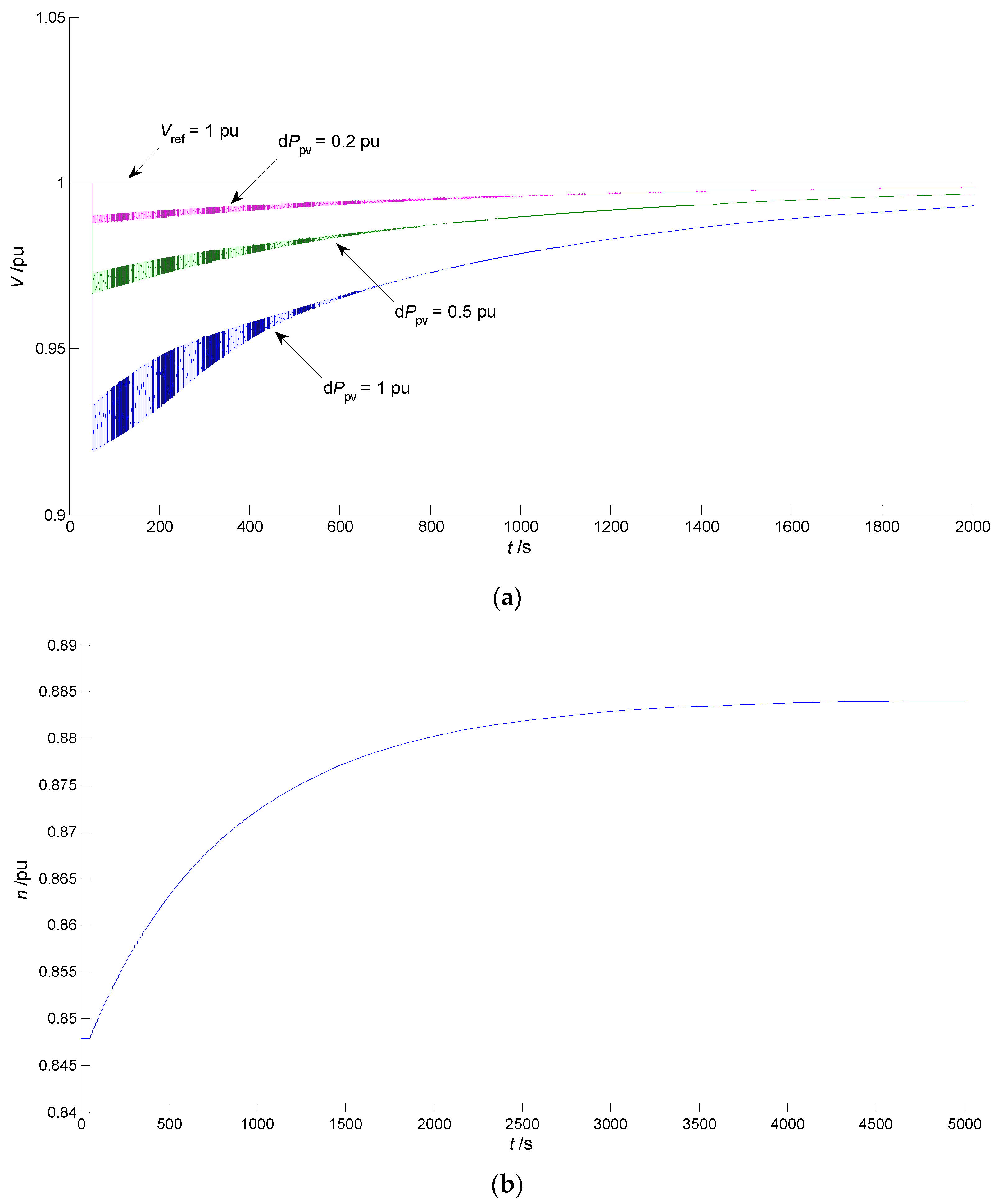
2.5.1. Sudden Drop of PV Power—Long-Term Voltage Recovery

Assume that the system shown in Figure 1 is operating at the SHB point H₁, the initial P_pv is 1 pu, and Q₁ is maintained at 10.3418 pu. Considering extremely bad weather conditions, such as a total solar eclipse, at time t = 50 s, P_pv suddenly drops from 1 pu to 0 pu, 0.5 pu, and 0.8 pu, respectively. The drop depth dP_pv is 1 pu, 0.5 pu, and 0.2 pu, respectively. It can be seen from Figure 5a that the load bus voltage V drops after the disturbance occurs, but an OLTC adjustment can finally recover V to near the target value V_ref (1 pu) after a long period of time. As shown in Figure 5b, the drop depth dP_pv is 1 pu and it is big enough. When the disturbance occurs, the transformation ratio n continues to increase to raise the load bus voltage and eventually stabilizes at a value of 0.884 pu after a very long time.

It can be determined by calculation that when P_pv drops suddenly, OLTC can all adjust V to near the target value, and V can be recovered faster under the smaller drop depth dP_pv.

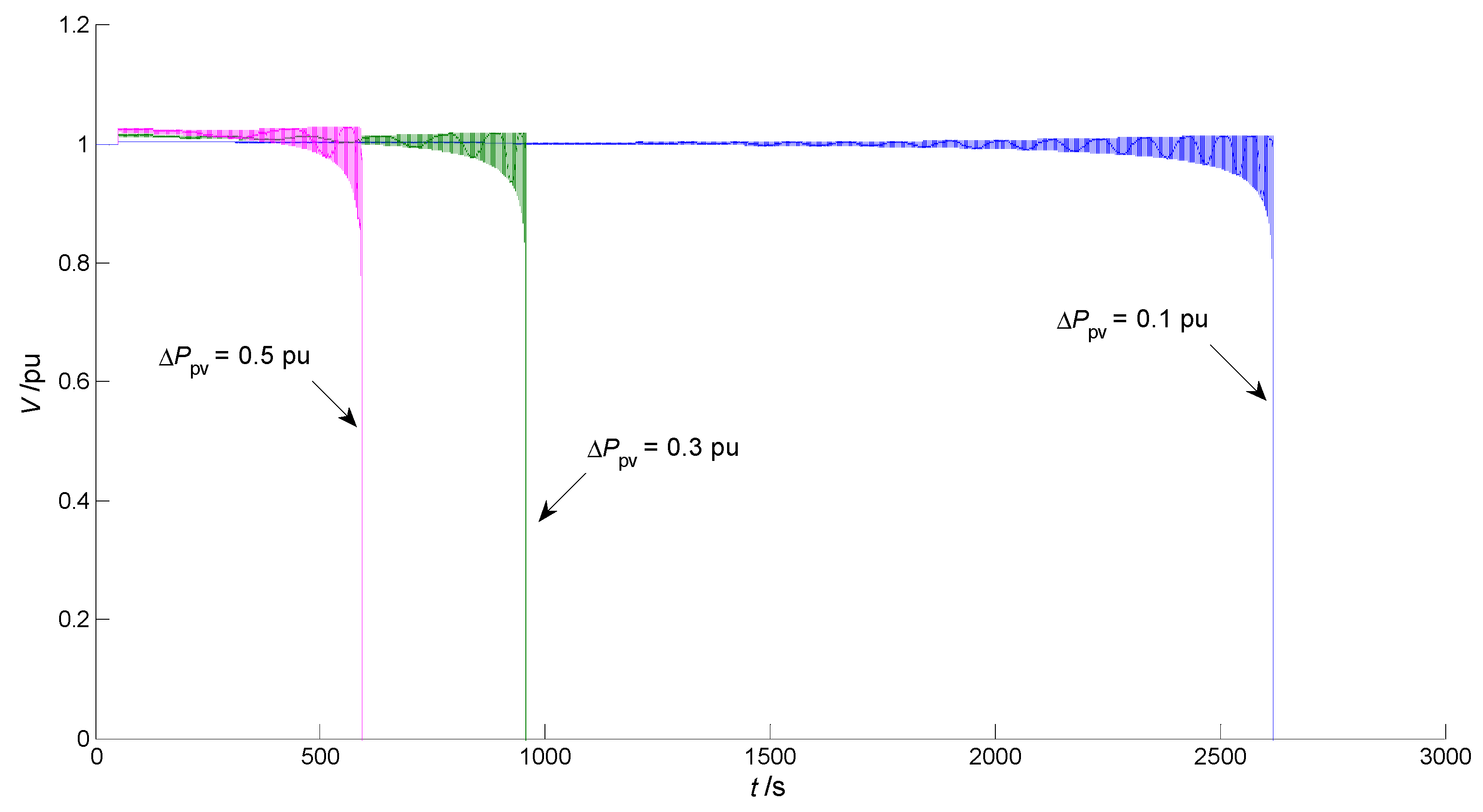
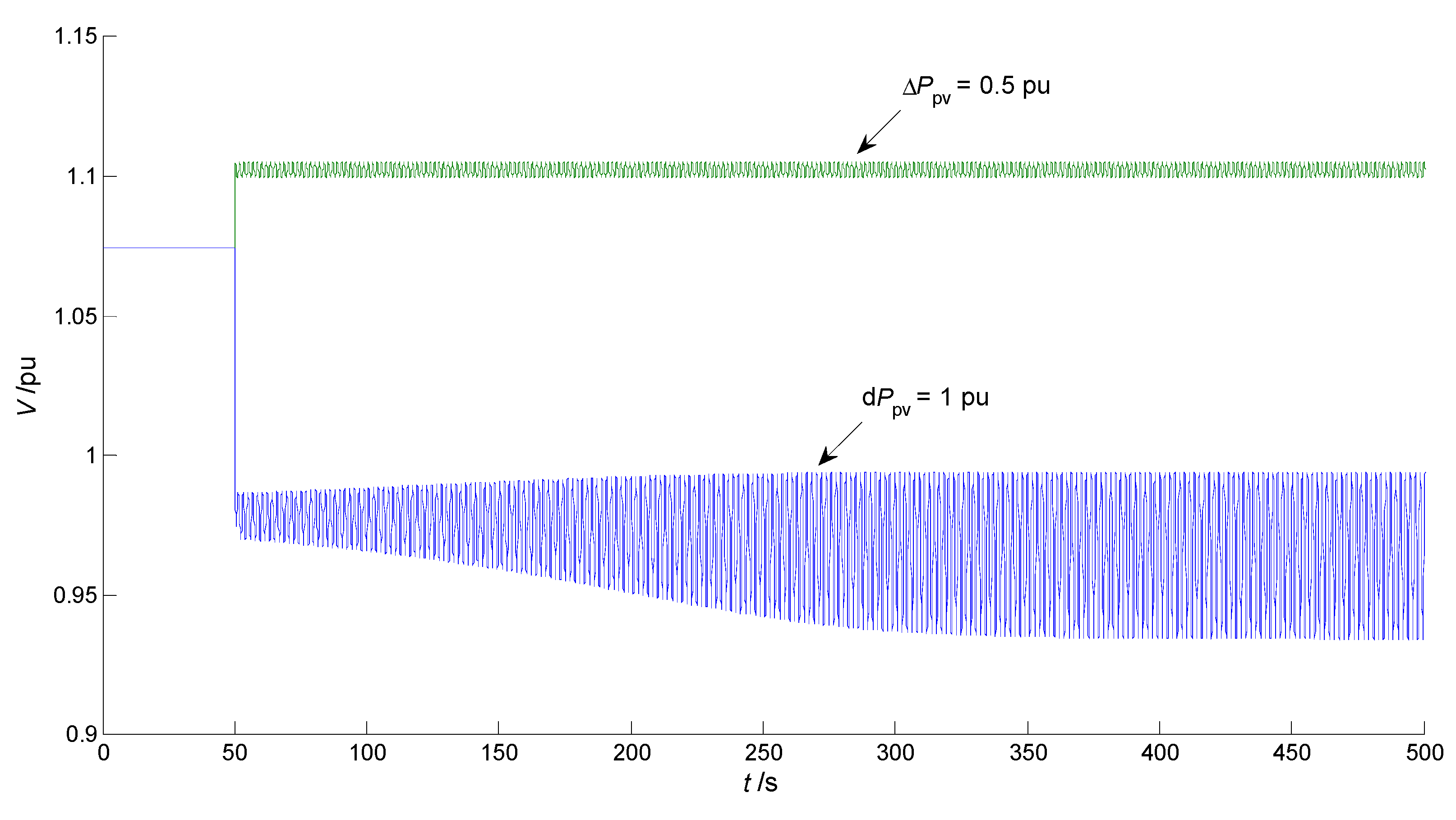
2.5.2. Sudden Increase in PV Power—Long-Term Voltage Collapse

Now assume that the system shown in Figure 1 is operating at the SHB point H₁, P_pv increases suddenly from 1 pu to 1.1 pu, 1.3 pu, and 1.5 pu, respectively. The increment ΔP_pv is 0.1 pu, 0.3 pu, and 0.5 pu, respectively. It can be seen from Figure 6 that the voltage V collapses after a long period of time. The larger ΔP_pv is, the faster V collapses, but the time frame is still in the category of long-term voltage stability.

According to the above analyses, in the absence of any control measures taken, P_pv is preferably not greater than the PV active power corresponding to the SHB point H₁ (P_pv.H1). In practice, P_pv is generally less than the PV-installed capacity P_pvN, hence a solution is to ensure that P_pvN ≤ P_pv.H1. However, this solution limits the use of PV power generation.

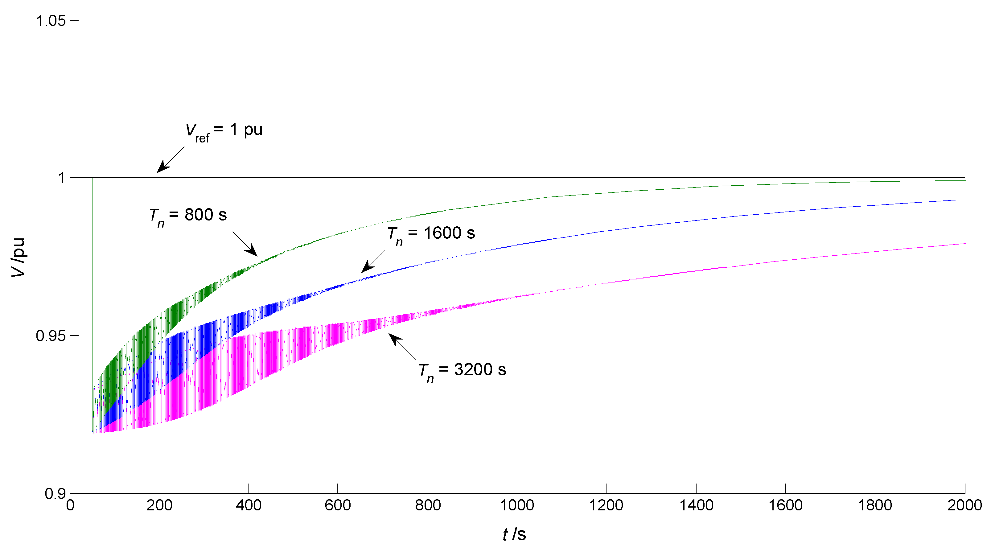
2.5.3. Impact of OLTC’s Time Constant—Key Influencing Factor Investigation

Different time constants T_n can make different impacts on long-term voltage stability when P_pv has a sudden change. In Figure 7, when P_pv drops from 1 pu to 0 pu, a smaller T_n is conducive to the recovery of the voltage V. However, in Figure 8, when P_pv increases from 1 pu to 1.3 pu, a smaller T_n is not conducive to voltage stability.

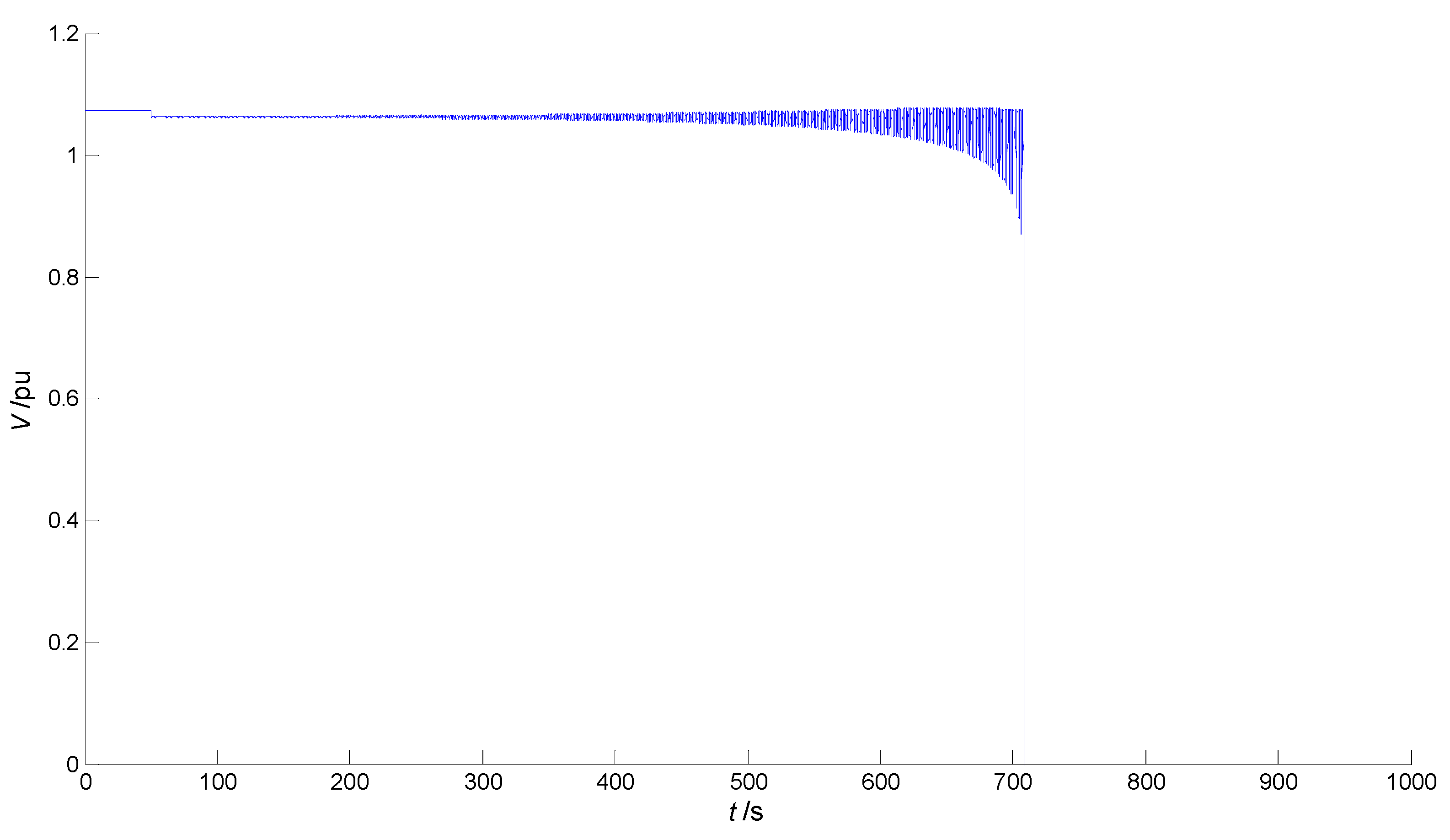
3. Comparison with the PV Grid-Connected 3-Bus System without OLTC

As shown in Figure 1, the PV grid-connected 3-bus system without OLTC is equivalent to the system with OLTC being locked in n = 1 pu, and the system’s ODEs take the first four equations of Equation (11) [24]. Keeping P_pv = 1 pu, the bifurcation calculation results show that on the stable half of the Q₁–V equilibrium point curve, there is a UHB point H₁ (corresponding to Q₁ = 11.1309 pu), a SHB point H₂ (corresponding to Q₁ = 11.4999 pu), and a SNB point LP (corresponding to Q₁ = 11.5069 pu) [24].

Taking the UHB point H₁ as the initial operating point, since it is a subcritical Hopf bifurcation point, a small sudden increase in the reactive load Q₁ can cause long-term voltage collapse. As shown in Figure 9, assuming that P_pv is maintained at 1 pu, Q₁ increases suddenly from 11.1309 pu to 11.1809 pu at time t = 50 s (namely ΔQ₁ = 0.05 pu), and the load bus voltage V collapses at about t = 708 s.

Compared with Figure 3a, due to the lack of OLTC adjustment, the time to reach voltage collapse has been reduced, but it still belongs in the category of long-term voltage stability.

Assume that Q₁ remains unchanged (keeping 11.1309 pu), and the impact of the sudden change of P_pv on long-term voltage stability is investigated. As shown in Figure 10, P_pv drops suddenly from 1 pu to 0 pu (namely dP_pv = 1 pu) at time t = 50 s. After V drops, the increasing oscillation is carried out firstly and the continuous oscillation (namely the constant-amplitude oscillation) begins at about t = 350 s after the disturbance occurs, and the oscillation amplitude of V is (0.9942 − 0.9344) × 100% = 5.98% > 5%. For the continuous oscillation, if the voltage’s oscillation amplitude is greater than or equal to 5%, it can be considered that the load bus is experiencing long-term voltage oscillation instability.

The smaller the drop depth dP_pv is, the longer the time for the voltage V to begin the continuous oscillation is, but the larger the oscillation amplitude of V will be [24]. For example, when P_pv suddenly drops from 1 pu to 0.8 pu (namely dP_pv = 0.2 pu), the time for the load voltage V to begin the continuous oscillation is about t = 4800 s after the disturbance occurs, and the oscillation amplitude of V reaches (1.072 − 0.8562) × 100% = 21.58% >> 5%.

On the other hand, as shown in Figure 10, when P_pv suddenly increases from 1 pu to 1.5 pu (namely ΔP_pv = 0.5 pu), after the voltage V increases, it quickly enters a continuous oscillation, and the oscillation amplitude is (1.105 − 1.099) × 100% = 0.6%, far less than 5%, which does not pose a threat to voltage stability.

The operation comparison results of the system with OLTC and without OLTC are listed in

Table 3. Comparison of the PV grid-connected 3-bus system with OLTC and without OLTC, taking the HB point H₁ as the initial operating point.

The Content of Comparison	With OLTC	Without OLTC
Bifurcation type of point H1	SHB	UHB
Reactive load Q1 of H1 (pu)	10.3418 pu	11.1309 pu
Voltage amplitude of H1 (pu)	1 pu (Vref)	1.0744 pu
Sudden small increase of Q1	Long-term voltage collapse	Long-term voltage collapse
Sudden drop of Ppv	Long-term voltage recovery	Long-term voltage oscillation instability (Oscillation amplitude ≥ 5%)
Sudden increase of Ppv	Long-term voltage collapse	Long-term voltage oscillation without instability (Oscillation amplitude << 5%)

. According to the comparative analyses, in order to avoid the long-term voltage oscillation instability when P_pv has a sudden drop, it is advisable to adopt the scheme of installing OLTC. For the sudden increase in P_pv, measures such as limiting the installed capacity of the PV station or locking OLTC can be used to solve the potential threat.

4. Design of the Index and Control Methods for Preventing Long-Term Voltage Collapse

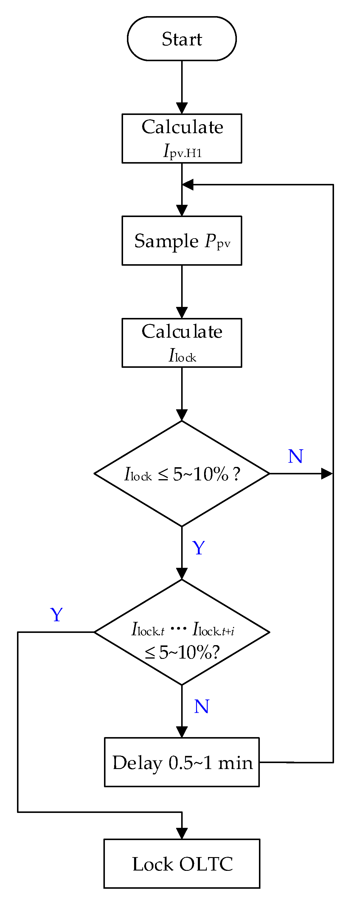
4.1. Prevention of Voltage Collapse Caused by a Sudden Increase in PV Power

For the 3-bus system with OLTC and PV shown in Figure 1, the installed capacity P_pvN can be limited according to the value of P_pv at the SHB point H₁ (P_pv.H1) so that P_pv does not exceed P_pv.H1. However, in practice, P_pvN may be much larger than P_pv.H1, so limiting the installed capacity is not an economic method.

In Figure 10 and Table 3, at the UHB point, when P_pv increases suddenly from 1 pu to 1.5 pu (ΔP_pv = 0.5 pu), long-term voltage oscillation with minimal amplitude will occur in the system without OLTC. Therefore, the locking OLTC method (namely maintaining a constant transformation ratio) can be used when P_pv increases suddenly in the system with OLTC, in order to prevent long-term voltage collapse.

For a better implementation of this locking OLTC method, a locking-OLTC index is designed:

$$I_{\mathrm{lock}}=1-\frac{P_{\mathrm{pv}}}{P_{\mathrm{pv}.\mathrm{H}1}}\le 5~10\%$$

(12)

Under the premise of a constant Q₁, where the value of the I_lock index is less than or equal to 0, OLTC should be locked in time. To keep a certain margin, the threshold can even be raised to 5~10%.

For example, when the system with OLTC operates at the SHB point H₁, assuming that Q₁ is maintained at Q_1.H1 and P_pv fluctuates, once the I_lock index value is less than or equal to 5~10%, the locking OLTC method can be used to avoid long-term voltage collapse.

Assume that the system with OLTC operates at the SHB point H₁, and Q₁ is maintained at 10.3418 pu. When P_pv increases suddenly from 1 pu to 1.1 pu, 1.3 pu, and 1.5 pu, respectively, I_lock is −0.1, −0.3, and −0.5, respectively. Now OLTC is locked in n = 0.9 pu, it can be seen from Figure 11 that V can quickly recover to an acceptable stable value.

The flow chart of the locking OLTC method is shown in Figure 12. Since the voltage collapse caused by the sudden increase in P_pv is a long process (up to hundreds of seconds or more), the method of locking OLTC is completely feasible.

Considering the fluctuation of P_pv, the I_lock index should be calculated and judged twice or even more consecutively, with a delay of 0.5~1 min between the two consecutive calculations and judgments. Once the two (or more) consecutive judgment results are the same, the command of locking OLTC should be issued, and n will be locked at a constant value.

4.2. Prevention of Voltage Collapse Caused by a Sudden Increase in Load Power

The traditional load-margin index [7] can be modified as follows:

$$I_{\mathrm{LMHB}}=1-\frac{Q_1}{Q_{1.\mathrm{H}1}}$$

(13)

where Q_1.H1 is the reactive power of the SHB point H₁.

Once the I_LMHB index value is less than 0, the load-shedding method can be taken to improve the load margin. A detailed load-shedding scheme is referred to in the literature [7]. Since the impact of the sudden increase in P_pv at the SHB point can be solved by using the locking OLTC method, the value of I_LMHB can be 0.

Load shedding is certainly a conservative method, and it may also cause a small-amplitude oscillation in the load bus voltage.

5. Conclusions

The typical 3-bus system containing an OLTC and a PV station is investigated for long-term voltage stability using bifurcation theory, and a new index and a locking OLTC method are used to prevent long-term voltage collapse. Using the bifurcation calculation and the time-domain calculation, and by comparison with the system without OLTC, the innovation conclusions are stated as follows:

(1) There are two SHB points and an SNB point on the stable half of the equilibrium point curve in the 3-bus system with OLTC and PV, and at the SHB point, a small sudden increase in reactive load power Q₁, or a sudden increase in PV active power P_pv can all cause long-term voltage collapse. This phenomenon suggests that SHB is also potentially threatening to the voltage stability.

(2) Aiming to change of P_pv at the SHB point suddenly, when P_pv drops suddenly, an OLTC adjustment can recover the load bus voltage to near the target value after a long period of time; when P_pv increases suddenly, locking OLTC and taking a suitable ration n can recover the voltage to a stable value. The impact of PV power disturbance at the SHB point on long-term voltage stability can be eliminated through the OLTC adjustment, and the system’s long-term voltage stability will focus on the impact of load power disturbance.

(3) The time constant T_n of OLTC is an important influencing factor in long-term voltage stability, as it can affect the process of long-term voltage collapse and long-term voltage recovery. However, under different disturbances, the magnitude of T_n can cause different effects.

(4) A new locking OLTC index I_lock based on PV active power was proposed. It can be taken as the benchmark of locking OLTC when P_pv increases suddenly at the SHB point. Moreover, a modified load-margin index I_LMHB is proposed to prevent long-term voltage collapse caused by the small sudden increase in load power at the SHB point.

Obviously, the discrete model of OLTC and the continuous changes of P_pv are not considered in the bifurcation analysis of the present case, and the calculation workload of bifurcation is very heavy for the multi-bus grid-connected system. The above topics require further study.

References

1. Zhou, X.; Zhao, Q.; Zhang, Y.; Sun, L. Integrated energy production unit: An innovative concept and design for energy transition toward low-carbon development. CSEE J. Power Energy Syst. 2021, 7, 1133–1139. [Google Scholar]
2. Guo, J.; Ma, S.; Wang, T.; Jing, Y.; Hou, W.; Xu, H. Challenges of developing a power system with a high renewable energy proportion under China’s carbon targets. iEnergy 2022, 1, 12–18. [Google Scholar]
3. Landera, Y.G.; Zevallos, O.C.; Neves, F.A.S.; Neto, R.C.; Prada, R.B. Control of PV systems for multimachine power system stability improvement. IEEE Access 2022, 10, 45061–45072. [Google Scholar]
4. Sajadi, A.; Rañola, J.A.; Kenyon, R.W.; Hodge, B.M.; Mather, B. Dynamics and stability of power systems with high shares of grid-following inverter-based resources: A tutorial. IEEE Access 2023, 11, 29591–29613. [Google Scholar]
5. Campanhol, L.B.G.; Silva, S.A.O.D.; Oliveira, A.A.D.; Bacon, V.D. Power flow and stability analyses of a multifunctional distributed generation system integrating a photovoltaic system with unified power quality conditioner. IEEE Trans. Power Electr. 2018, 34, 6241–6256. [Google Scholar]
6. Kawabe, K.; Ota, Y.; Yokoyama, A.; Tanaka, K. Novel dynamic voltage support capability of photovoltaic systems for improvement of short-term voltage stability in power systems. IEEE Trans. Power Syst. 2017, 32, 1796–1804. [Google Scholar]
7. Li, S.; Wei, Z.; Ma, Y. Fuzzy load-shedding strategy considering photovoltaic output fluctuation characteristics and static voltage stability. Energies 2018, 11, 779. [Google Scholar]
8. Rahman, S.; Saha, S.; Islam, S.N.; Arif, M.T.; Mosadeghy, M.; Haque, M.E.; Oo, A.M.T. Analysis of power grid voltage stability with high penetration of solar PV systems. IEEE Trans. Ind. Appl. 2021, 57, 2245–2257. [Google Scholar]
9. Li, S.; Lu, Y.; Ge, Y. Static voltage stability zoning analysis based on a sensitivity index reflecting the influence degree of photovoltaic power output on voltage stability. Energies 2023, 16, 2808. [Google Scholar]
10. General Administration of Quality Supervision, Inspection and Quarantine of the People’s Republic of China; Standardization Administration of the People’s Republic of China. Code on Security and Stability for Power System (GB 38755–2019); Standards Press of China: Beijing, China, 2019; p. 13.
11. Khoshkhoo, H.; Yari, S.; Pouryekta, A.; Ramachandaramurthy, V.K.; Guerrero, J.M. A remedial action scheme to prevent mid/long-term voltage instabilities. IEEE Syst. J. 2021, 15, 923–934. [Google Scholar]
12. Islam, S.R.; Sutanto, D.; Muttaqi, K.M. Coordinated decentralized emergency voltage and reactive power control to prevent long-term voltage instability in a power system. IEEE Trans. Power Syst. 2015, 30, 2591–2603. [Google Scholar]
13. Sun, Q.; Cheng, H.; Song, Y. Bi-Objective reactive power reserve optimization to coordinate long- and short-term voltage stability. IEEE Access 2018, 6, 13057–13065. [Google Scholar]
14. Matavalam, A.R.R.; Singhal, A.; Ajjarapu, V. Monitoring long term voltage instability due to distribution & transmission interaction using unbalanced μPMU & PMU measurements. IEEE Trans. Smart Grid. 2020, 11, 873–883. [Google Scholar]
15. Matavalam, A.R.R.; Ajjarapu, V. Long term voltage stability Thevenin index using voltage locus method. In Proceedings of the 2014 IEEE PES General Meeting, National Harbor, MD, USA, 27–31 July 2014; pp. 1–5. [Google Scholar]
16. Wang, C.; Ju, P.; Wu, F.; Lei, S.; Pan, X. Long-term voltage stability-constrained coordinated scheduling for gas and power grids with uncertain wind power. IEEE Trans. Sustain. Energy 2022, 13, 363–377. [Google Scholar]
17. Dharmapala, K.D.; Rajapakse, A.; Narendra, K.; Zhang, Y. Machine learning based real-time monitoring of long-term voltage stability using voltage stability indices. IEEE Access 2020, 8, 222544–222555. [Google Scholar]
18. Cai, H.; Ma, H.; Hill, D.J. A data-based learning and control method for long-term voltage stability. IEEE Trans. Power Syst. 2020, 35, 3203–3212. [Google Scholar]
19. Yang, H.; Qiu, R.C.; Tong, H. Reconstruction residuals based long-term voltage stability assessment using autoencoders. J. Mod. Power Syst. Clean Energy 2020, 8, 1092–1093. [Google Scholar]
20. Peng, Z.; Hu, G.; Han, Z. Dynamic analysis of the power system voltage stability affected by OLTC. Proc. CSEE 1999, 19, 61–65, 78. [Google Scholar]
21. Sun, Y.; Wang, Z. Modeling of OLTC and its impact on the voltage stability. Autom. Electr. Power Syst. 1998, 22, 10–13. [Google Scholar]
22. Londero, R.R.; Affonso, C.d.M.; Vieira, J.P.A. Long-term voltage stability analysis of variable speed wind generators. IEEE Trans. Power Syst. 2015, 30, 439–447. [Google Scholar]
23. Munkhchuluun, E.; Meegahapola, L. Impact of the solar photovoltaic (PV) generation on long-term voltage stability of a power network. In Proceedings of the 2017 IEEE Innovative Smart Grid Technologies-Asia (ISGT-Asia), Auckland, New Zealand, 4–7 December 2017; pp. 1–6. [Google Scholar]
24. Li, S.; Wei, Z.; Sun, G.; Gao, P.; Xiao, J. Voltage stability bifurcation of large-scale grid-connected PV system. Electr. Power Autom. Equip. 2016, 36, 17–23. [Google Scholar]
25. Li, S.; Wei, Z.; Ma, Y.; Cheng, J. Prediction and control of Hopf bifurcation in a large-scale PV grid-connected system based on an optimised support vector machine. J. Eng. 2017, 14, 2666–2671. [Google Scholar] [CrossRef]
26. Canizares, C.A.; Mithulananthan, N.; Milano, F.; Reeve, J. Linear performance indices to predict oscillatory stability problems in power systems. IEEE Trans. Power Syst. 2004, 19, 1104–1114. [Google Scholar] [CrossRef]
27. Cutsem, T.V.; Vournas, C. Bifurcations. In Voltage Stability of Electric Power Systems; Springer: New York, NY, USA, 1998; pp. 153–160. [Google Scholar]
28. Wang, Y.; Chen, H.; Zhou, R. A nonlinear controller design for SVC to improve power system voltage stability. Int. J. Electr. Power Energy Syst. 2000, 22, 463–470. [Google Scholar]
29. Jing, Z.; Xu, D.; Chang, Y.; Chen, L. Bifurcations, chaos, and system collapse in a three node power system. Int. J. Electr. Power Energy Syst. 2003, 25, 443–461. [Google Scholar]
30. Tamimi, B.; Cañizares, C.; Bhattacharya, K. System stability impact of large-scale and distributed solar photovoltaic generation: The case of Ontario, Canada. IEEE Trans. Sustain. Energy 2013, 4, 680–688. [Google Scholar] [CrossRef]
31. Li, S.; Wei, Z.; Sun, G.; Wang, Z. Stability research of transient voltage for multi-machine power systems integrated large-scale PV power plant. Acta Energiae Solaris Sin. 2018, 39, 3356–3362. [Google Scholar]
32. Bao, L.; Duan, X.; He, Y. Analysis of the effect of OLTC on the voltage stability through time domain simulation. J. Huazhong Univ. Sci. Tech. 2000, 28, 61–63. [Google Scholar]
33. Duan, X.; He, Y.; Chen, D. Dynamic analysis of the relation between on-load tap changer and voltage stability. Autom. Electr. Power Syst. 1995, 19, 14–19. [Google Scholar]
Figure 1. The 3-bus system with OLTC and PV. (a) The initial model. (b) The simplified model.
Energies 16 06383 g001
Figure 2. The equilibrium point curves. (a) Q1n curve (Ppv = 1 pu). (b) Ppvn curve (Q1 = 10.3418 pu).
Energies 16 06383 g002
Figure 3. The time-domain change curves when Q1 increases suddenly from the SHB point H1 (Tn = 1600 s). (a) tV curves at different increments of Q1. (b) tn curve (ΔQ1 = 0.05 pu).
Energies 16 06383 g003
Figure 4. tV curves at different time constants of OLTC when Q1 increases suddenly from the SHB point H1Q1 = 0.05 pu).
Energies 16 06383 g004
Figure 5. The time-domain change curves when Ppv drops suddenly from the SHB point H1 (Tn = 1600 s). (a) tV curves at different drop depths of Ppv. (b) tn curve (dPpv = 1 pu).
Energies 16 06383 g005
Figure 6. tV curves when Ppv increases suddenly from the SHB point H1 (Tn = 1600 s).
Energies 16 06383 g006
Figure 7. tV curves at different time constants of OLTC when Ppv drops suddenly from the SHB point H1 (dPpv = 1 pu).
Energies 16 06383 g007
Figure 8. tV curves at different time constants of OLTC when Ppv increases suddenly from the SHB point H1Ppv = 0.3 pu).
Energies 16 06383 g008
Figure 9. tV curve when Q1 increases suddenly from the UHB point H1Q1 = 0.05 pu).
Energies 16 06383 g009
Figure 10. tV curves when Ppv changes suddenly from the UHB point H1 (dPpv = 1 pu and ΔPpv = 0.5 pu).
Energies 16 06383 g010
Figure 11. tV curves when Ppv changes suddenly from the SHB point H1 (OLTC is locked in n = 0.9 pu).
Energies 16 06383 g011
Figure 12. The flow chart of the locking OLTC method (t and i are the sampling time and times).
Energies 16 06383 g012