


Energy Assessment of Different Powertrain Options for Heavy-Duty Vehicles and Energy Implications of Autonomous Driving †


Abstract
:1. Introduction
2. Materials and Methods
2.1. Vehicle Use Case
2.2. Driving Cycle Determination
2.3. Vehicle Parametrisation
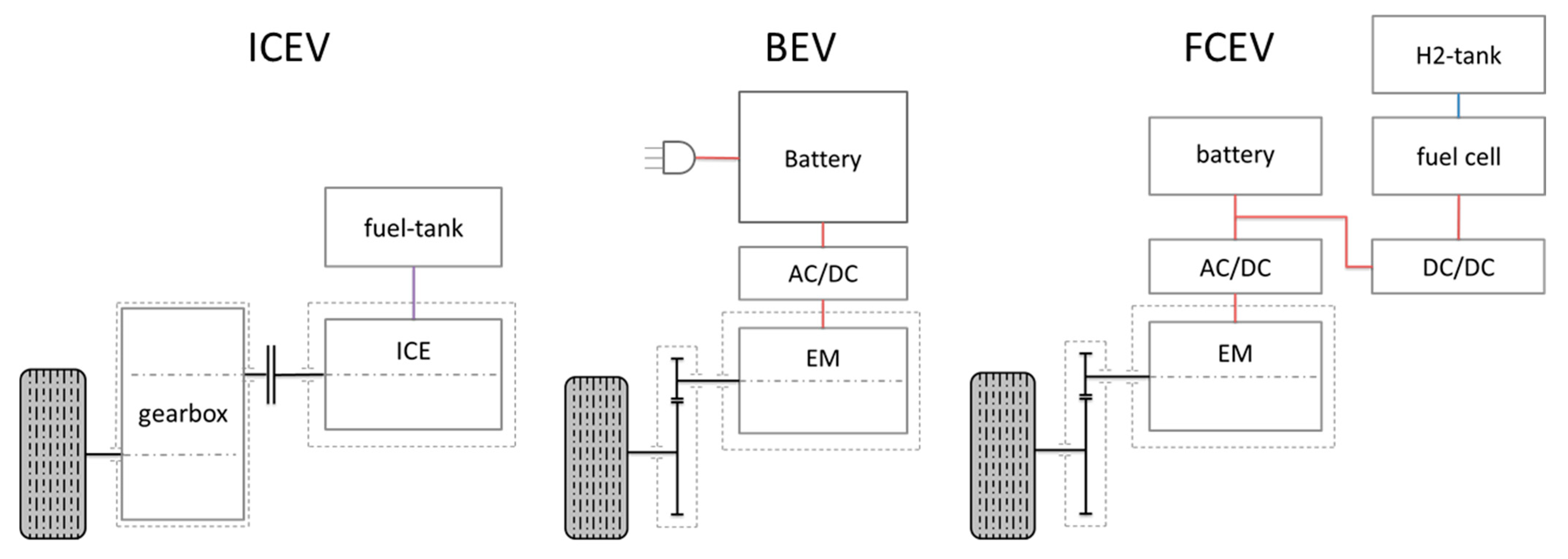
2.4. Powertrain Design
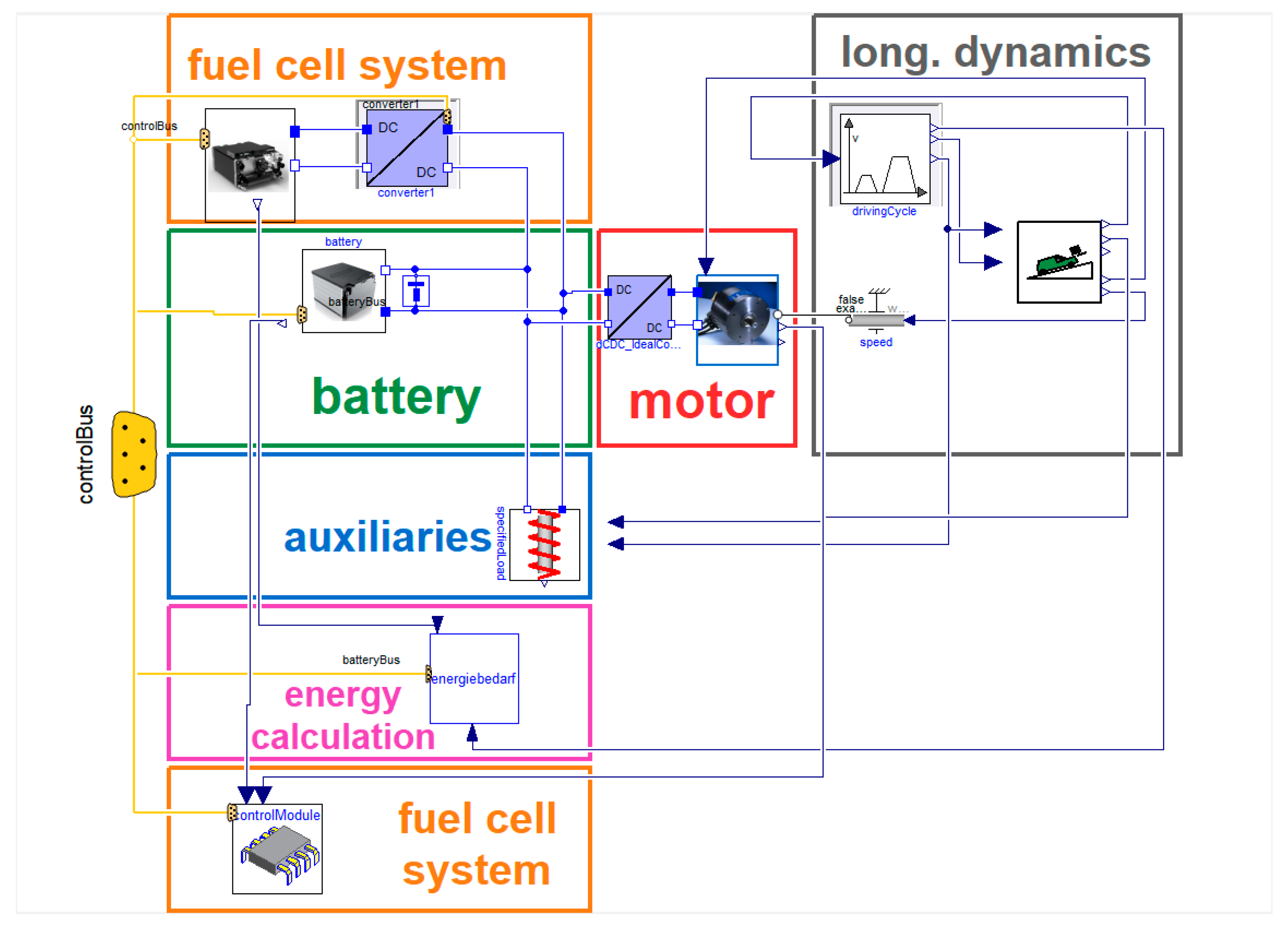
2.5. Simulation Concept
2.6. Modelling
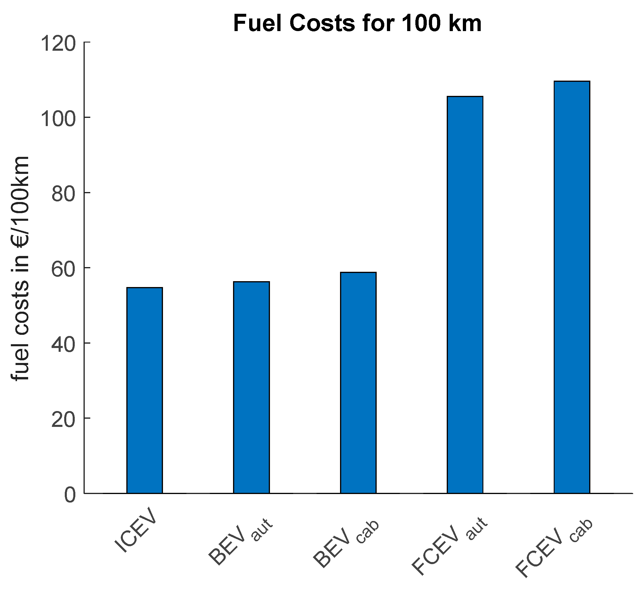
2.7. Method for the Calculation of Primary Energy, CO2 Emissions, and Fuel Costs
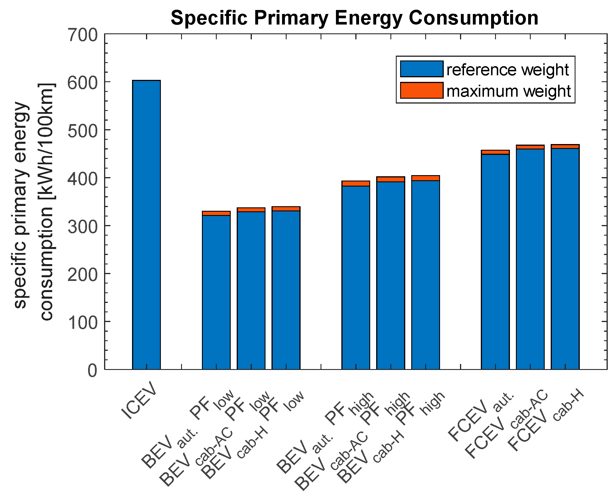
3. Results
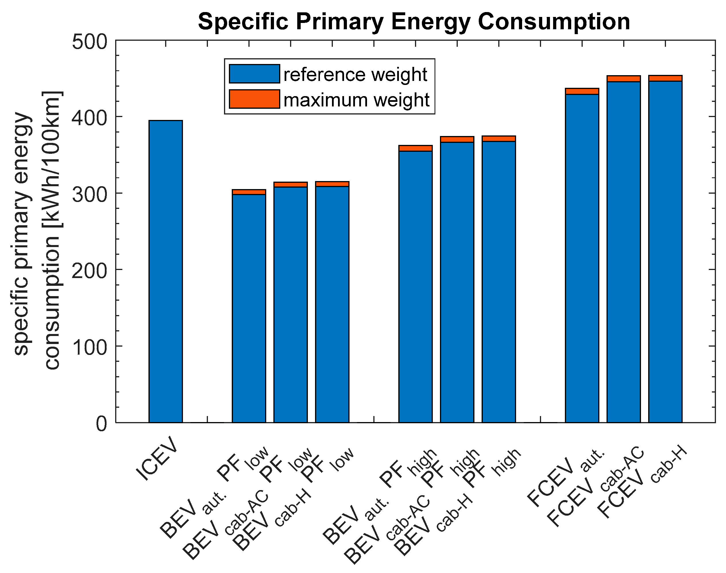
3.1. FIGE Cycle
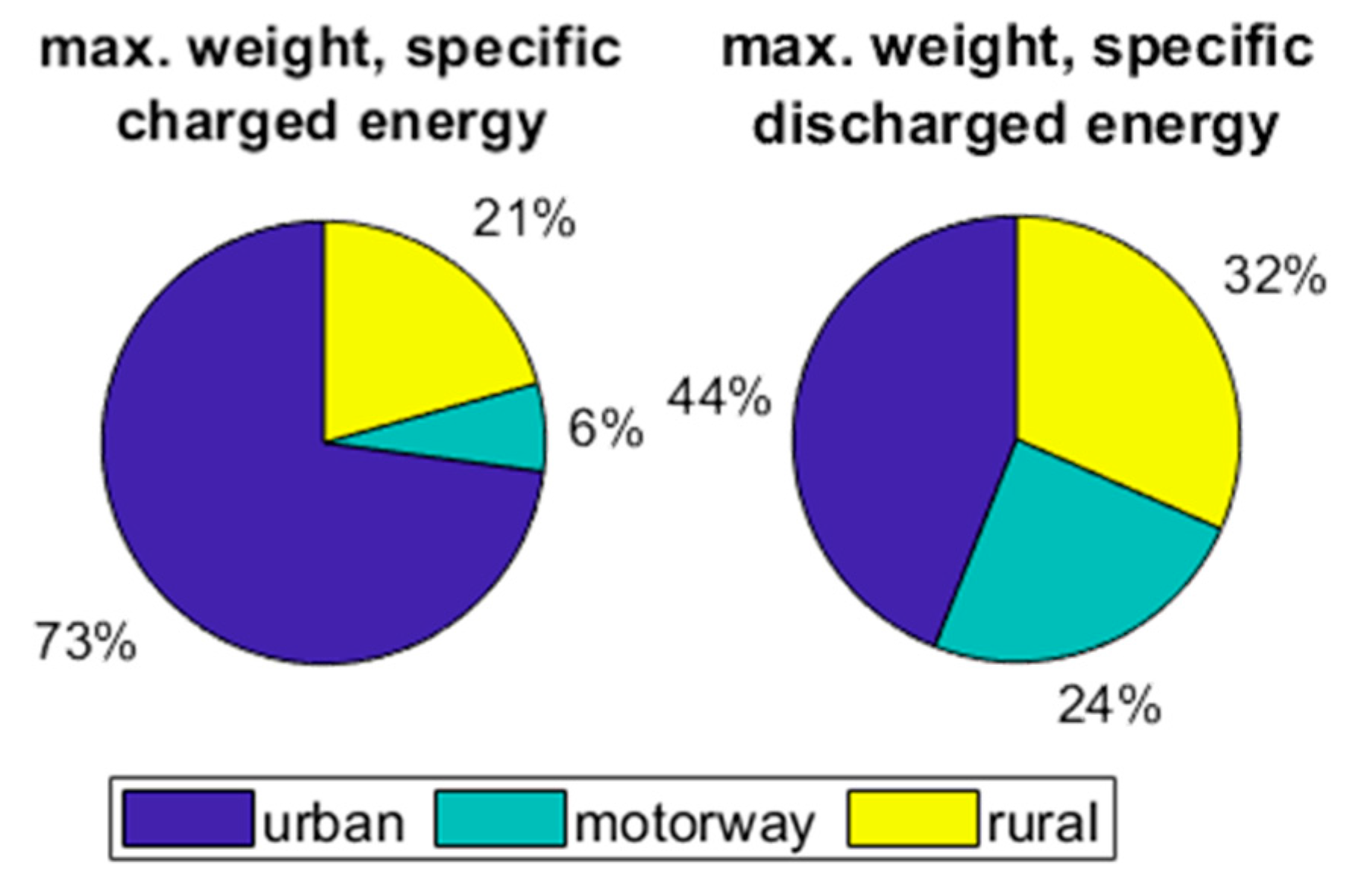
3.2. Daycycle
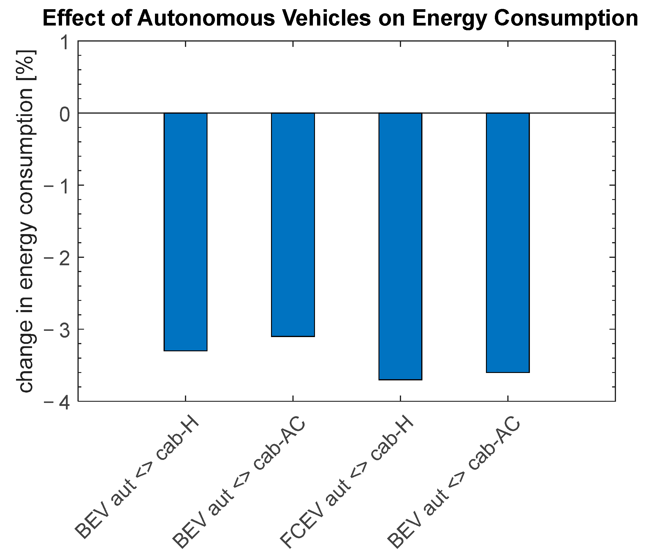
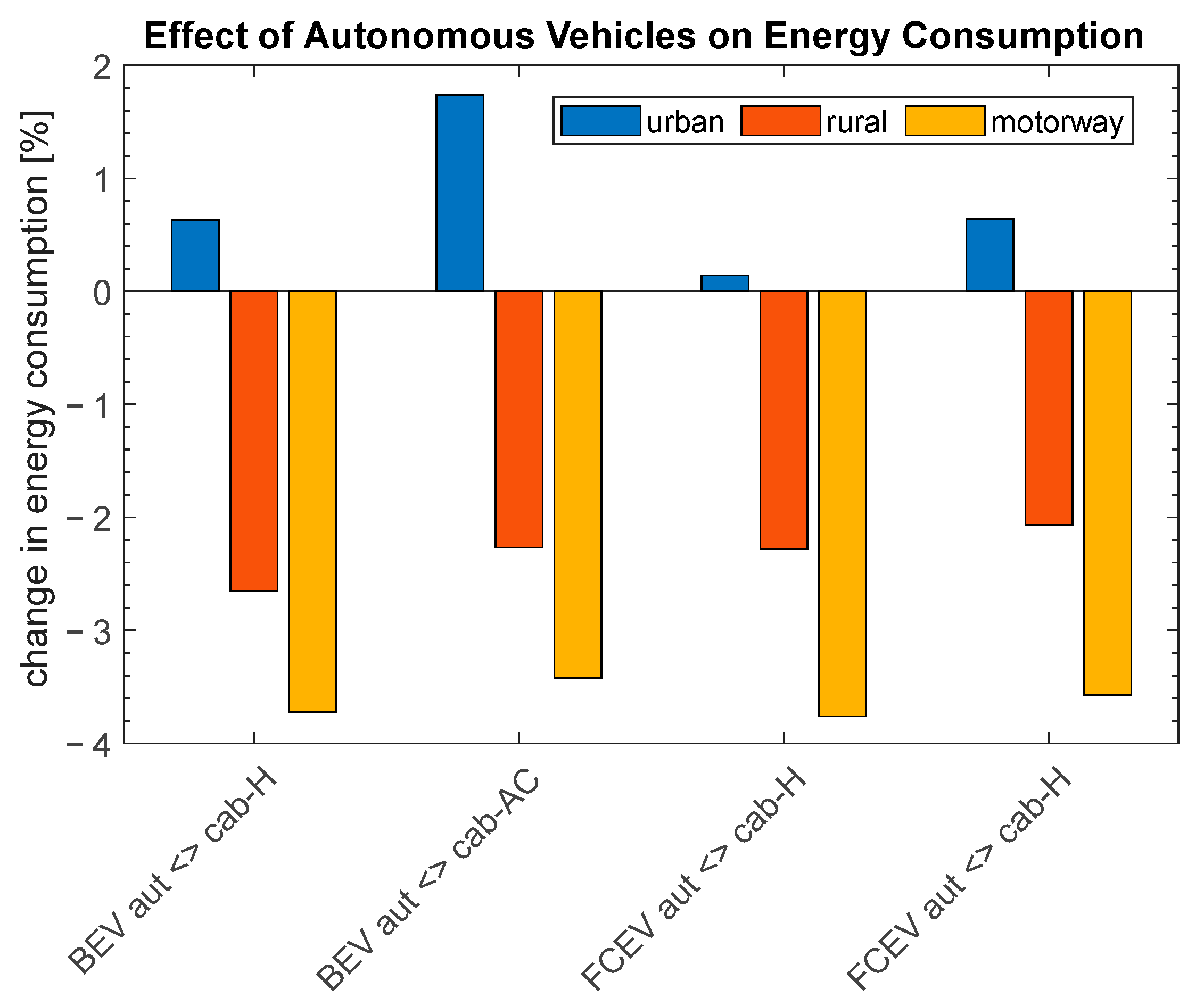
3.3. Autonomous Driving
4. Discussion
Author Contributions
Funding
Data Availability Statement
Acknowledgments
Conflicts of Interest
References
- Statistisches Bundesamt. Europäischer Green Deal: Klimaneutralität bis 2050. Available online: https://www.destatis.de/Europa/DE/Thema/GreenDeal/GreenDeal.html (accessed on 27 July 2023).
- ACEA. Fuel Types of New Trucks: Electric 0.6%, Diesel 96.6% Market Share Full-Year 2022. Available online: https://www.acea.auto/files/ACEA_Trucks_by_fuel_type_full-year-2022.pdf (accessed on 27 July 2023).
- European Council. Verordnung (EU) 2019/des Europäischen Parlaments und des Rates vom 20. Juni 2019 zur Festlegung von CO2-Emissionsnormen für Neue Schwere Nutzfahrzeuge und zur Änderung der Verordnungen (EG) Nr. 595/2009 und (EU) 2018/956 des Europäischen Parlaments und des Rates sowie der Richtlinie 96/53/EG des Rates; European Council: Strasbourg, France, 2019. [Google Scholar]
- Transport & Environment. Die Dekarbonisierung des Lkw-Fernverkehrs in Deutschland. Ein Vergleich der Verfügbaren Antriebstechnologien und Ihrer Kosten. Available online: https://www.transportenvironment.org/wp-content/uploads/2021/07/2021_04_TE_Dekarbonisierung_des_Lkw_Fernverkehrs_in_Deutschland_kurzfassung_final.pdf (accessed on 27 July 2023).
- Sharpe, B.E.; Muncrief, R. Literature Review: Real-World Fuel Consumption of Heavy-Duty Vehicles in the United States, China, and the European Union; International Council on Clean Transportation: Washington, DC, USA, 2015; pp. 1–27. [Google Scholar]
- Broekaert, S.; Fontaras, G. CO2 Emissions of the European Heavy-Duty Vehicle: Analysis of the 2019–2020 Reference Year Data; Publications Office of the European Union: Luxembourg, 2022; ISBN 978-92-76-49854-4. [Google Scholar]
- European Commission. Vehicle Energy Consumption Calculation TOol—VECTO. Available online: https://climate.ec.europa.eu/eu-action/transport-emissions/road-transport-reducing-co2-emissions-vehicles/vehicle-energy-consumption-calculation-tool-vecto_en (accessed on 14 July 2023).
- Cunanan, C.; Tran, M.-K.; Lee, Y.; Kwok, S.; Leung, V.; Fowler, M. A Review of Heavy-Duty Vehicle Powertrain Technologies: Diesel Engine Vehicles, Battery Electric Vehicles, and Hydrogen Fuel Cell Electric Vehicles. Clean Technol. 2021, 3, 474–489. [Google Scholar] [CrossRef]
- Jöhrens, J. Vergleichende Analyse der Potentiale von Antriebstechnologien für Lkw im Zeithorizont 2030; IFEU: Heidelberg, Germany, 2022. [Google Scholar]
- Jöhrens, J.; Allekotte, M.; Heining, F.; Helms, H.; Räder, D.; Schillinger, M.; Thienel, M.; Dürrbeck, K.; Schwemmer, M.; Köllermeier, N.; et al. Potentialanalyse für Batterie-Lkw-Teilbericht im Rahmen des Vorhabens “Elektrifizierungspotenzial des Güter-und Busverkehrs-My eRoads; IFEU: Heidelberg, Germany, 2021. [Google Scholar]
- Basma, H.; Beys, Y.; Rodriguez, F. Battery Electric Tractor-Trailers in the European Union: A Vehicle Technology Analysis; International Council on Clean Transportation: Washington, DC, USA, 2021. [Google Scholar]
- Basma, H.; Rodriguez, F. Fuel Cell Electric Tractor-Trailers: Technology Overview and Fuel Economy; Working Paper; International Council on Clean Transportation: Washington, DC, USA, 2022; Volume 23. [Google Scholar]
- Åhman, M. Primary energy efficiency of alternative powertrains in vehicles. Energy 2001, 26, 973–989. [Google Scholar] [CrossRef]
- Basma, H.; Zhou, Y.; Rodriguez, F. Fuel-Cell Hydrogen Long-Haul Trucks in Europe: A Total Cost of Ownership Analysis; ICCT White Paper; International Council on Clean Transportation: Washington, DC, USA, 2022. [Google Scholar]
- Catherine, R.; Subhrajit, G. Autonomous Vehicles and Energy Impacts: A Scenario Analysis. Energy Procedia 2017, 143, 47–52. [Google Scholar] [CrossRef]
- Chen, B.; Chen, Y.; Wu, Y.; Xiu, Y.; Fu, X.; Zhang, K. The Effects of Autonomous Vehicles on Traffic Efficiency and Energy Consumption. Systems 2023, 11, 347. [Google Scholar] [CrossRef]
- Islam, E.S.; Moawad, A.; Kim, N.; Rousseau, A. Vehicle Electrification Impacts on Energy Consumption for Different Connected-Autonomous Vehicle Scenario Runs. World Electr. Veh. J. 2020, 11, 9. [Google Scholar] [CrossRef]
- Hahn, R. New exterior design options for improving the efficiency of fully autonomous heavy duty vehicles. In Proceedings of the 2022 Second International Conference on Sustainable Mobility Applications, Renewables and Technology (SMART), Cassino, Italy, 23–25 November 2022; IEEE: New York, NY, USA, 2022; pp. 1–5, ISBN 978-1-6654-7146-6. [Google Scholar]
- Schall, P.; Sigle, S.; Ulrich, C. Design Strategy for a Distributed Energy Storage in a Modular Mover. In Proceedings of the 2021 Sixteenth International Conference on Ecological Vehicles and Renewable Energies (EVER), Monte-Carlo, Monaco, 5–7 May 2021; IEEE: New York, NY, USA, 2021; pp. 1–5, ISBN 978-1-6654-4902-1. [Google Scholar]
- Sigle, S.; Hahn, R. Energy Consumption Comparison of Current Powertrain Options in Autonomous Heavy Duty Vehicles (HDV). In Proceedings of the 2022 Second International Conference on Sustainable Mobility Applications, Renewables and Technology (SMART), Cassino, Italy, 23–25 November 2022; IEEE: New York, NY, USA, 2022; pp. 1–7, ISBN 978-1-6654-7146-6. [Google Scholar]
- Delgado, O.; Rodriguez, F.; Muncrief, R. Fuel Efficiency Technology in European Heavy-Duty Vehicles: Baseline and Potential for the 2020–2030 Timeframe; International Council on Clean Transportation: Washington, DC, USA, 2017. [Google Scholar]
- Wolf, A. Modell zur Straßenbautechnischen Analyse der Durch den Schwerverkehr Induzierten Beanspruchung des BAB-Netzes: [Bericht zum Forschungsprojekt F 1100.3406002 des Arbeitsprogramms der Bundesanstalt für Straßenwesen]; Wirtschaftsverl. NW, Verl. für Neue Wiss: Bremerhaven, Germany, 2010; ISBN 9783869180014. [Google Scholar]
- Mercedes-Benz. Data Sheet Actros 2046 LS 4x2 BM 96340212; Mercedes-Benz: Stuttgart, Germany, 2023. [Google Scholar]
- Earl, T.; Mathieu, L.; Cornelis, S.; Kenny, S.; Ambel, C.C.; Nix, J. Analysis of long haul battery electric trucks in EU. In Proceedings of the 8th Commercial Vehicle Workshop, Graz, Austria, 17–18 May 2018; Graz University of Technology: Graz, Austria, 2018. [Google Scholar]
- European Union. Directive 96/53/EC—Authorised Dimensions and Weights for Trucks, Buses and Coaches Involved in International Traffic; European Union: Brussels, Belgium, 1996. [Google Scholar]
- Fontaras, G.; Grigoratos, T.; Savvidis, D.; Anagnostopoulos, K.; Luz, R.; Rexeis, M.; Hausberger, S. An experimental evaluation of the methodology proposed for the monitoring and certification of CO2 emissions from heavy-duty vehicles in Europe. Energy 2016, 102, 354–364. [Google Scholar] [CrossRef]
- Jeschke, S. Grundlegende Untersuchungen von Elektrofahrzeugen im Bezug auf Energieeffizienz und EMV mit Einer Skalierbaren Power-HiL-Umgebung; University of Duisburg-Essen: Duisburg, Germany, 2016. [Google Scholar]
- Weustenfeld, T. Heiz- und Kühlkonzept für ein Batterieelektrisches Fahrzeug Basierend auf Sekundärkreisläufen. Ph.D. Dissertation, Technische Universität Braunschweig, Braunschweig, Germany, 2018. [Google Scholar]
- Hoepke, E.; Breuer, S. Nutzfahrzeugtechnik; Springer Fachmedien Wiesbaden: Wiesbaden, Germany, 2016; ISBN 978-3-658-09536-9. [Google Scholar]
- Braig, T.; Dittus, H.; Ungethüm, J.; Engelhardt, T. The Modelica library ‘AlternativeVehicles’ for vehicle system simulation. Simul. Notes Eur. SNE 2012, 22, 101–106. [Google Scholar]
- Sigle, S.; Epple, F.; Dongus, P. Investigation of the Applicability of a Two-Motor Concept for Public Transportation Systems. In Proceedings of the 2021 Sixteenth International Conference on Ecological Vehicles and Renewable Energies (EVER), Monte-Carlo, Monaco, 5–7 May 2021; IEEE: New York, NY, USA, 2021; pp. 1–6, ISBN 978-1-6654-4902-1. [Google Scholar]
- Konz, M.; Lemke, N.; Försterling, S.; Eghtessad, M. Spezifische Anforderungen an das Heiz-Klimasystem Elektromotorisch Angetriebener Fahrzeuge. FAT-Schriftenreihe. 2011, p. 233. Available online: https://d-nb.info/1053546009/34 (accessed on 16 November 2022).
- BDEW Bundesverband der Energie- und Wasserwirtschaft e.V. Grundlagenpapier Primärenergiefaktoren: Zusammenhänge von Primärenergie und Endenergie in der Energetischen Betrachtung. Fakten und Argumente. 2022. Available online: https://www.bdew.de/media/documents/Awh_20221124_BDEW-Grundlagenpapier_PEF_final.pdf (accessed on 12 July 2023).
- Balaras, C.A.; Dascalaki, E.G.; Psarra, I.; Cholewa, T. Primary Energy Factors for Electricity Production in Europe. Energies 2023, 16, 93. [Google Scholar] [CrossRef]
- Frischknecht, R.; Tuchschmid, M. Primärenergiefaktoren von Energiesystemen; ESU-Services GmbH, Fair Consulting in Sustainability, Uster: Schaffhausen, Switzerland, 2008. [Google Scholar]
- ADAC. Spritpreis-Entwicklung: Benzin- und Dieselpreise Seit 1950. Available online: https://www.adac.de/verkehr/tanken-kraftstoff-antrieb/deutschland/kraftstoffpreisentwicklung/ (accessed on 14 July 2023).
- Verivox. Strompreis Stand 12.07.2023. Available online: https://www.verivox.de/strom/strompreise (accessed on 12 July 2023).
- H2 Mobility. Unsere Wasserstoffpreise an H2 Mobility Wasserstofftankstellen: H2 Truck Fuel. Available online: https://h2-mobility.de/ (accessed on 14 July 2023).
- Klell, M.; Eichlseder, H.; Trattner, A. Wasserstoff in der Fahrzeugtechnik: Erzeugung, Speicherung, Anwendung, 4; Aktualisierte und Erweiterte Auflage; Springer Vieweg: Wiesbaden, Germany, 2018; ISBN 9783658204471. [Google Scholar]
- European Environment Agency. Greenhouse Gas Emission Intensity of Electricity Generation. Available online: https://www.eea.europa.eu/data-and-maps/daviz/co2-emission-intensity-13/#tab-googlechartid_chart_11 (accessed on 11 July 2023).
- Xia, X.; Hashemi, E.; Xiong, L.; Khajepour, A. Autonomous Vehicle Kinematics and Dynamics Synthesis for Sideslip Angle Estimation Based on Consensus Kalman Filter. IEEE Trans. Control Syst. Technol. 2023, 31, 179–192. [Google Scholar] [CrossRef]
- Xia, X.; Bhatt, N.P.; Khajepour, A.; Hashemi, E. Integrated Inertial-LiDAR-Based Map Matching Localization for Varying Environments. IEEE Trans. Intell. Veh. 2023, 1–12. [Google Scholar] [CrossRef]
- Liu, W.; Xia, X.; Xiong, L.; Lu, Y.; Gao, L.; Yu, Z. Automated Vehicle Sideslip Angle Estimation Considering Signal Measurement Characteristic. IEEE Sens. J. 2021, 21, 21675–21687. [Google Scholar] [CrossRef]
- Xia, X.; Meng, Z.; Han, X.; Li, H.; Tsukiji, T.; Xu, R.; Zheng, Z.; Ma, J. An automated driving systems data acquisition and analytics platform. Transp. Res. Part C Emerg. Technol. 2023, 151, 104120. [Google Scholar] [CrossRef]


| Parameter | ICEV | BEV | FCEV |
|---|---|---|---|
| chassis tractor | 3867 kg | 3867 kg | 3867 kg |
| +mechanical powertrain ICE | 3000 kg | ||
| +battery | 5887 kg | 910 kg | |
| +power electronics, e-motor | 400 kg | 400 kg | |
| +fuel cell | 125 kg | ||
| +hydrogen tank | 1275 kg | ||
| +trailer (empty) | 7000 kg | 7000 kg | 7000 kg |
| =Curb weight | 13,867 kg | 17,154 kg | 13,577 kg |
| Reference weight | 40,000 kg | 40,000 kg | 40,000 kg |
| Maximum weight | 40,000 kg | 42,000 kg | 42,000 kg |
| payload (max. weight − curb weight) | 26,133 kg | 24,846 kg | 28,423 kg |
| Auxiliary Consumers | Vehicle with Driver Cabin [W] | Vehicle without Driver Cabin [W] |
|---|---|---|
| radio | 20 | - |
| instrument lighting | 20 | - |
| heated windshield | 60 | - |
| electric heating | 1000 | - |
| electric air conditioner compressor max. power | (3000) | - |
| parking light | 7 | 7 |
| low beam | 90 | 90 |
| turn signal light | 90 | 90 |
| windscreen wiper | 10 | 10 |
| license plate light | 25 | 25 |
| brake light | 11 | 11 |
| fog light | 20 | 20 |
| rear fog light | 2 | 2 |
| turn signal | 5 | 5 |
| electric power steering pump | 1800 | 1800 |
| electric air compressor | 4500 | 4500 |
| power of sensors | - | 2500 |
| total | 7660–9660 | 9060 |
| Description | Character | Unit | Value |
|---|---|---|---|
| Vehicle mass | mv | [kg] | 42,000 |
| Gravitational acceleration | g | [m/s2] | 9.81 |
| Rolling resistance coefficient | cr | [-] | 0.006 |
| Drag coefficient cabin vehicle | cw | [-] | 0.6 |
| Drag coefficient autonomous vehicle | cw | [-] | 0.52 |
| Front face | Af | [m2] | 9.615 |
| Air density | ρ | [kg/m3] | 1.2041 |
| Parameter | Unit | Heating | Cooling |
|---|---|---|---|
| temperature cabin | [°C] | 22.00 | 22.00 |
| ambient temperature | [°C] | 3.78 | 26.49 |
| ambient humidity | [%] | 72.48 | 46.80 |
| solar radiation constant | [Wm2] | 134.16 | 524.87 |
| Powertrain | Weight | Steering Type | Cabin |
|---|---|---|---|
| BEV | reference weight | autonomous | - |
| driver | heating | ||
| cooling | |||
| maximum weight | autonomous | - | |
| driver | heating | ||
| cooling | |||
| FCEV | reference weight | autonomous | - |
| driver | heating | ||
| cooling | |||
| maximum weight | autonomous | - | |
| driver | heating | ||
| cooling | |||
| ICEV | maximum weight = reference weight | driver | cooling |
| End Energy Source | Primary Energy Factor | Source |
|---|---|---|
| diesel | 1.22 | [35] |
| electricity low PF | 2.1 | [34] |
| electricity high PF | 2.5 | [34] |
| hydrogen | 1.46 | [33] |
Disclaimer/Publisher’s Note: The statements, opinions and data contained in all publications are solely those of the individual author(s) and contributor(s) and not of MDPI and/or the editor(s). MDPI and/or the editor(s) disclaim responsibility for any injury to people or property resulting from any ideas, methods, instructions or products referred to in the content. |
© 2023 by the authors. Licensee MDPI, Basel, Switzerland. This article is an open access article distributed under the terms and conditions of the Creative Commons Attribution (CC BY) license (https://creativecommons.org/licenses/by/4.0/).
Share and Cite
Sigle, S.; Hahn, R. Energy Assessment of Different Powertrain Options for Heavy-Duty Vehicles and Energy Implications of Autonomous Driving. Energies 2023, 16, 6512. https://doi.org/10.3390/en16186512
Sigle S, Hahn R. Energy Assessment of Different Powertrain Options for Heavy-Duty Vehicles and Energy Implications of Autonomous Driving. Energies. 2023; 16(18):6512. https://doi.org/10.3390/en16186512
Chicago/Turabian StyleSigle, Sebastian, and Robert Hahn. 2023. "Energy Assessment of Different Powertrain Options for Heavy-Duty Vehicles and Energy Implications of Autonomous Driving" Energies 16, no. 18: 6512. https://doi.org/10.3390/en16186512
APA StyleSigle, S., & Hahn, R. (2023). Energy Assessment of Different Powertrain Options for Heavy-Duty Vehicles and Energy Implications of Autonomous Driving. Energies, 16(18), 6512. https://doi.org/10.3390/en16186512