Abstract
For highly heterogeneous complex carbonate reef reservoirs, rock typing with respect to depositional conditions, secondary processes, and permeability and porosity relationships is a useful tool to improve reservoir characterization, modeling, prediction of reservoir volume properties, and estimation of reserves. A review of various rock typing methods has been carried out. The basic methods of rock typing were applied to a carbonate reservoir as an example. The advantages and disadvantages of the presented methods are described. A rock typing method based on a combination of hydraulic flow units and the R35 method is proposed. Clustering methods for rock typing are used. The optimum clustering method is identified, and for each rock type, the permeability–porosity relationships are built and proposed for use in the geomodelling stage.
1. Introduction
Carbonate reservoirs are characterized by a high heterogeneity of void space. The heterogeneity is caused by both abrupt changes in facies depositional conditions and widespread secondary processes that partially or completely rearrange the internal structure. The secondary changes are often selective. Reservoir properties can vastly vary both vertically and horizontally. Predicting properties in the reservoir interwell space is very important. Many studies address this issue, including facies analysis, determination of depositional conditions, rock typing, and sequence stratigraphy [1].
Identifying zones with different secondary processes and, hence, with different reservoir properties is essential for understanding reservoir structure and its static modeling. Detailed distribution of properties plays a significant role in calculating reserves, static and dynamic reservoir model preparation, planning geological and engineering activities, etc. The relationship between geological heterogeneity, reservoir quality, and reservoir performance [2] is paramount. Understanding these key relationships enables effective reservoir management [3].
The relationship between reservoir performance and quality is mostly fully reflected by permeability. Permeability is the most important property that determines fluid filtration in a reservoir. Many studies focused on permeability predictions in the interwell space [4,5]. For terrigenous reservoirs, permeability predictions in the interwell zone are simpler tasks than for carbonate reservoirs [6,7,8]. For terrigenous reservoirs, the standard approach with core-well-log correlation identification and property interpolation using geostatistic methods usually shows satisfied results of permeability distribution across reservoir volume [9]. For a complex carbonate reservoir, the problem of permeability distribution across the volume is extremely difficult [10,11]. Different approaches or their combinations are used for complex carbonate reservoir permeability predictions: rock typing, multi-scale data combining, seismotypes identification, scale effect estimation, anisotropy study, uncertainties analysis, etc. [12,13,14,15]. The permeability parameter is determined from various sources: core samples, well-test studies, nuclear magnetic resonance, acoustic logging, and others. The results of core studies are usually combined with logging curves to predict permeability in intervals without coring. However, for carbonate reservoirs, this prediction is generally ineffective. For more reliable predictions of permeability and reservoir quality, rock typing is used [16,17,18].
G. Archie [19] was one of the first to propose the definition of a rock type: a rock strata whose parts were deposited under the same conditions and were subjected to the same secondary transformation processes (fracture, cementation, or dissolution). A particular rock type must have a specific pore size distribution and, therefore, individual capillary pressure curves. The pore size distribution controls porosity and is related to permeability and water saturation [20].
There are many different approaches for typing carbonate reservoirs. The division into rock types is based on different physical characteristics of the rock: its hydraulic flow units (HFU), pore space geometry and structure, pore channel size, type and size of grains, their relation to the binder mass, etc. [21]. The hydraulic flow unit method is widely used for typing the carbonate reservoirs [22,23,24]. A hydraulic flow unit is an interval with certain properties prevailing in a reservoir. These intervals are controlled by both geological and petrophysical attributes that enable the prediction of reservoir characteristics. Accordingly, the diagenetic transformations prevailing in a particular part of the reservoir are an essential parameter controlling the hydraulic flow units [2]. The method is also applicable for rock typing in geological and dynamic modeling [25,26]. The method is based on the calculation of an integrated parameter—a flow zone indicator (FZI). However, there are uncertainties associated with combining hydraulic flow units into classes. Various techniques, such as GHE, machine learning, and the discrete rock typing (DRT) method, are used for this purpose [21,22].
A rather common method is to identify rock types based on pore channel size (Winland) [27,28]. Typing by pore channel radius has been proposed [29]:
- -
- Macropores (2 µm < R35 < 10 µm);
- -
- Mesopores (0.5 µm < R35 < 2 µm);
- -
- Micropores (0.1 µm < R35 < 0.5 µm).
In [30], it is proposed to distinguish rock types by calculating pore geometry (PG) and pore structure (PS). The calculated parameters are plotted on one graph in a bi-logarithmic scale, and the points lying on one straight line will correspond to one class. As the class increases, the quality of the reservoir will increase. The classification of P.W. Choquette and L.C. Pray is a classical lithological classification. It includes the following characteristics: basic porosity types, genetic factors, grain size, and grain number factors [31]. Another common classification is the approach developed by R.J. Dunham [32]. It is a structural classification that considers the following factors: the presence and type of form elements or grains, their relationship with the binder mass, and the structure of the binder mass. The Archie classification is based on the study of the structural features of the rock matrix and the nature of the visible void space. G.E. Archie studied a significant amount of actual data to show that the rock types are characterized by certain petrophysical properties (porosity, permeability, capillary pressure, and electrical resistivity), well-logging results, and petrophysical relationships. In other words, a comprehensive approach to rock-type identification is necessary [19]. The authors [33,34,35] have proposed an approach based on the analysis of accumulated correlations between porosity and permeability, enabling the estimation of the porosity–permeability relationship as the void space increases. Lorenz curves have been successfully used to assess reservoir heterogeneity [36,37]. Lorenz curves are also widely used in classifying reservoirs by void type. By highlighting sharp changes in the plot, it is possible to account for the inclusion of highly permeable intervals or fractures.
Thus, a review of the main rock typing methods shows that for the purposes of geological and dynamic models and permeability modeling in the reservoir volume, the methods based on the permeability and porosity relationships are the most applicable. These methods are based on hydraulic flow units, pore channel radius, and Lorenz curves, but the methods are rather generalized and need to be adapted to the peculiarities of a particular reservoir.
This study will typify the reservoir of Alpha oilfield using different methods, perform a comparison of these methods, propose an approach to rock typing using machine learning methods (clustering), identify the best method, and build dependencies to predict the permeability of different rock types.
2. Geological Settings
The Alpha field is located in the Timan-Pechora oil and gas province, on the territory of the Denisovsky Depression (Figure 1). Reef structures were widespread in the area during the Yelets and Zadonian times.
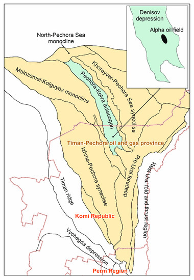
Figure 1.
Region tectonic map (Alpha oilfield location).
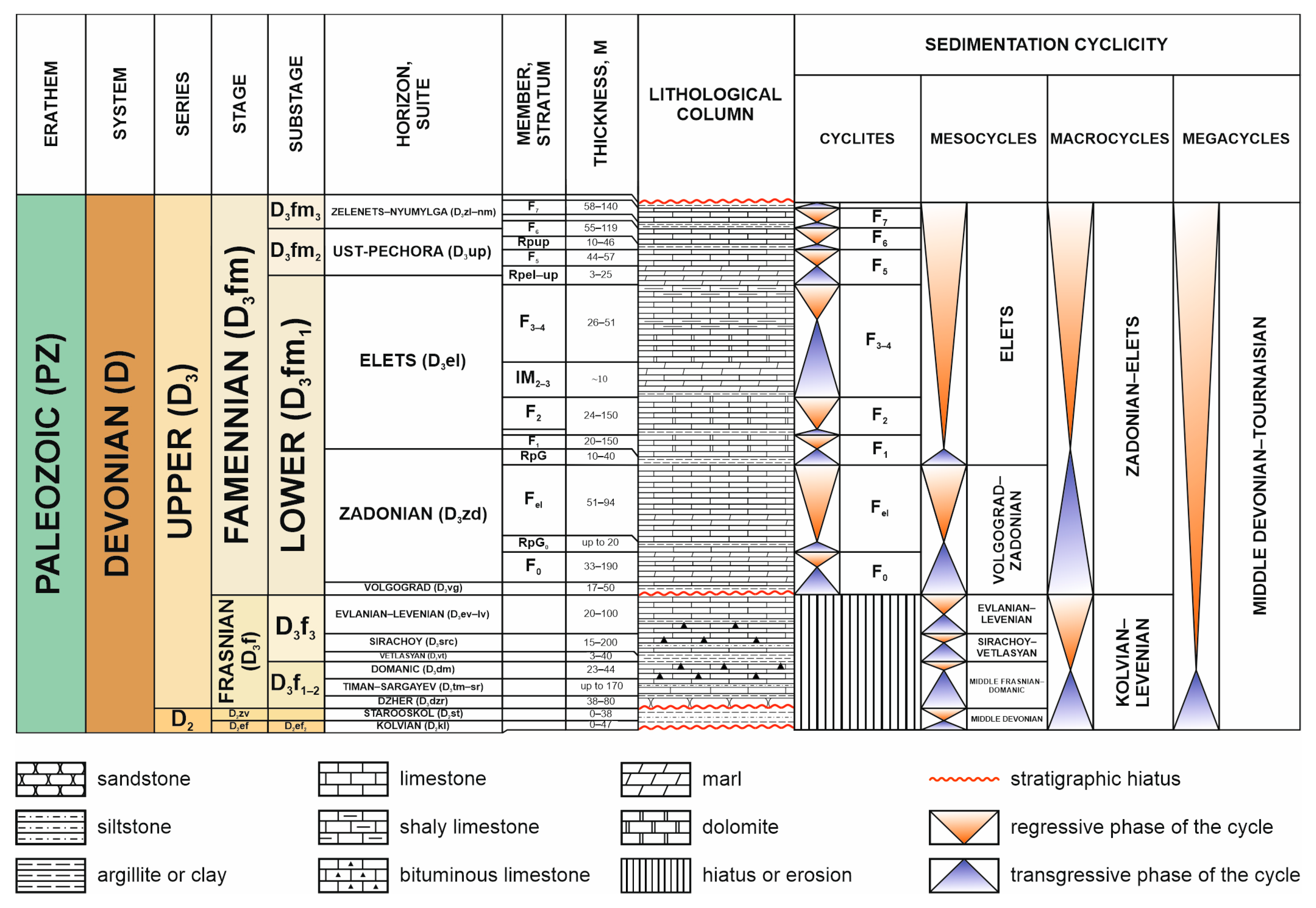
Rocks of carbonate strata of the Yelets and Zadonian age (Devonian) are characterized by core predominantly in their upper part (D3el) (Figure 2). According to the core, the formation is mostly limestone with areas of abundant secondary dolomitization. Leaching is widespread, with caverns of various sizes ranging from leaching pores to large voids up to several centimeters in diameter. Leaching has also been observed in limestones, but cavernosity is particularly strong in dolomites.
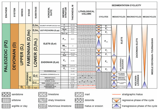
Figure 2.
Regional stratigraphic column.
Tilting and sub-vertical fracturing are presented, but often, the tilting fractures are resistive and impermeable, which are characterized by the upper part of the sequence. Sub-horizontal fractures are abundant in the upper part of the sequence and mostly remain open, even when naturally occurring.
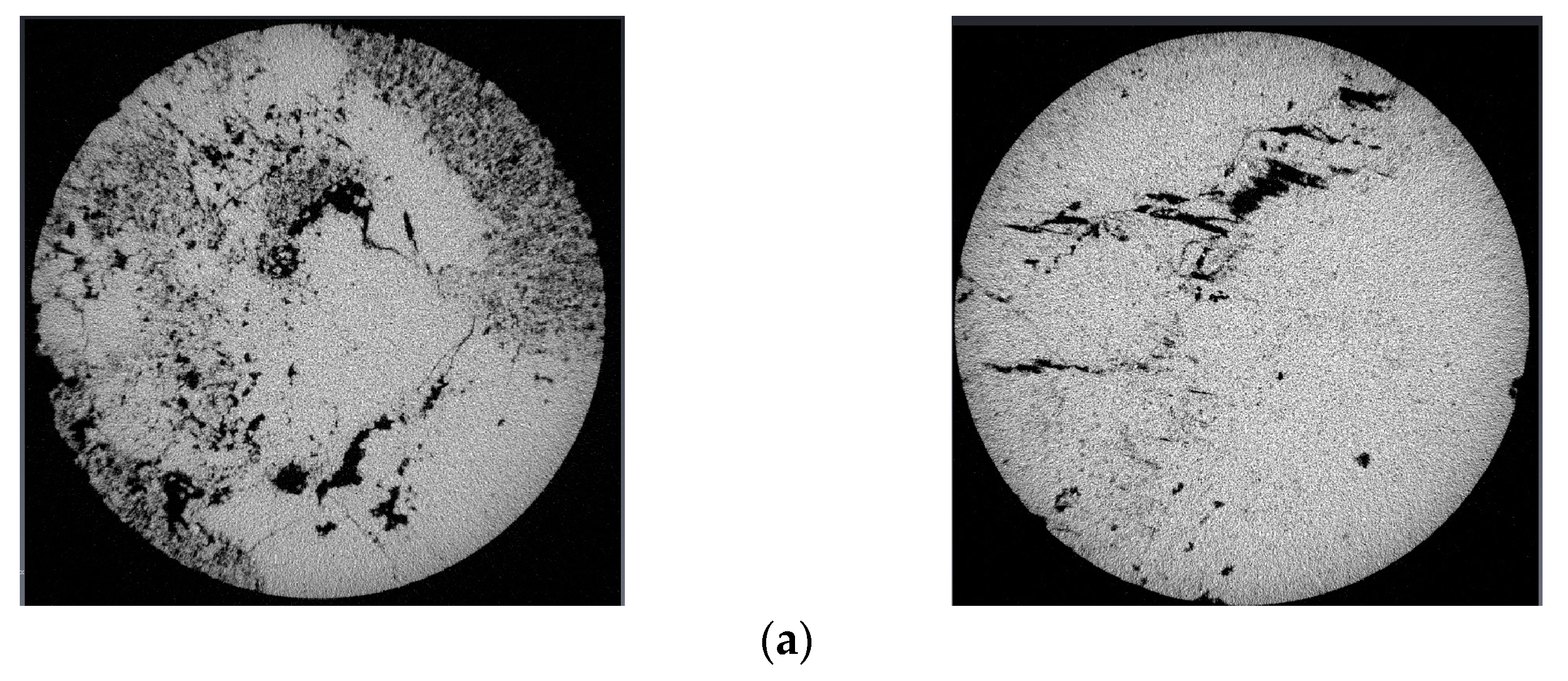
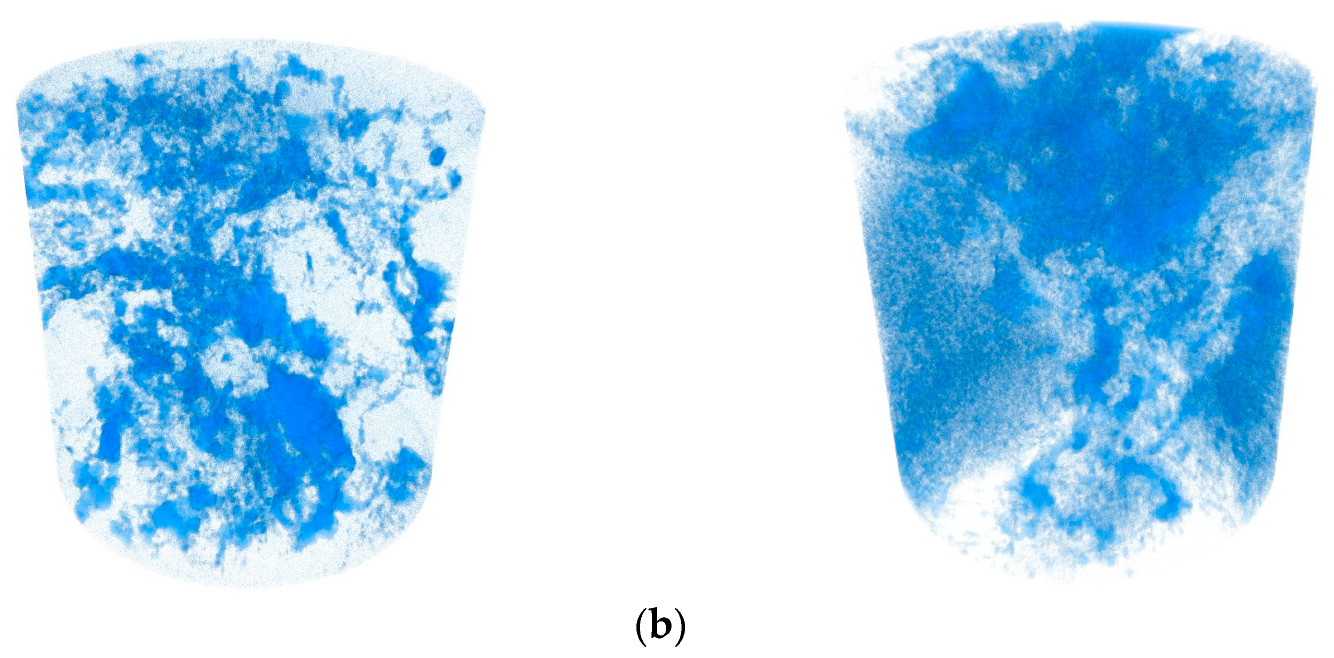
The reservoir rocks are classified as fracture-cavernous and pore-cavernous. Given the widespread development of leaching pores, all reservoirs in the section can be classified as a pore-fracture-cavernous type (Figure 3). Accordingly, caverns are the main part of pore space in the reservoir.
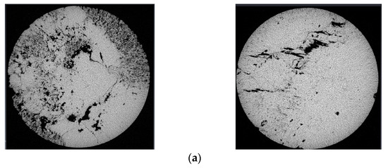
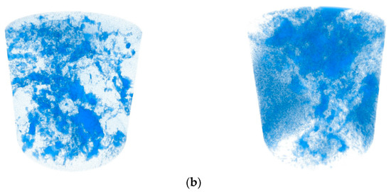
Figure 3.
Example of core samples (Yelets strata) with fracture-cavernous type (tomography results): (a) XY view; (b) 3D pore space view.
The range of porosity varies from 1 to 18.3%. Permeability varies from 0.001 to 722.8 (mD), with an average value of 20.3 (mD).
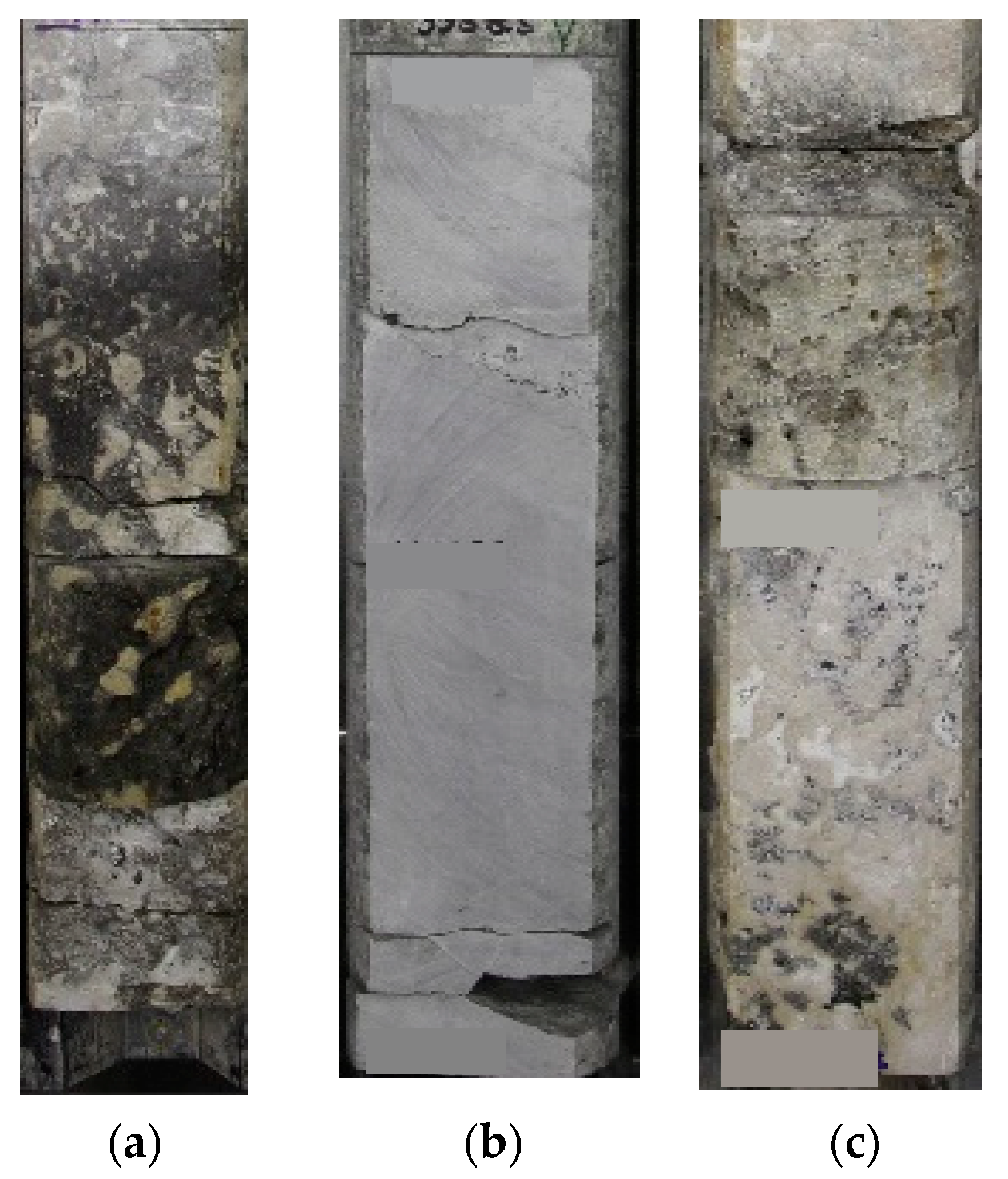
According to the lithological description of the core samples, three lithotypes are distinguished: microbial limestones, peloid limestones, and secondary dolomites (Figure 4). Microbial limestones are characterized by a clotted granular microstructure and areas with fenestrae and are partially dolomitized, stylolitized, porous, cavernous-porous, and fractured. Secondary processes are noted—calcitization, recrystallization, sulfatization, dolomitization, and rarely, pyritization. Peloid limestones consist of peloids, interclasts, and ooids. Stylolitization and fracturing are observed. Secondary dolomites are medium-coarse-grained, porous, and cavernous-porous.
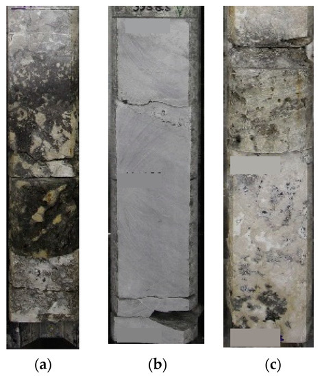
Figure 4.
Examples of lithotypes: (a) microbial limestones; (b) peloid limestones; and (c) secondary dolomites.
3. Materials and Methods
This study used various methods for rock typing of core samples (461 core samples) based on the assessment of permeability and porosity relationships.
The hydraulic flow unit method is based on calculating a complex parameter—the flow zone indicator (FZI) (1):
where RQI is the reservoir quality index, µm, and φz is the normalized porosity index, u.f.
RQI is defined by the equation:
where Kpr is the permeability coefficient, mD, and Kp is the porosity coefficient, u.f.
Φz describes the ratio of the void volume to the solid rock volume and is defined by the equation:
It is assumed that when RQI and φz values are plotted on a bi-logarithmic scale, sample points with close FZI values will be located near the same straight line and, thus, be characterized by similar pore channel features and, thus, form a hydraulic flow unit. Different approaches exist for combining and grouping points into one class: cluster analysis, neural networks, cumulative frequency analysis, discrete type method, and global hydraulic unit class method. In the first stage, the global hydraulic unit classes (GHE) method is proposed, which suggests establishing class boundaries based on the generalization of a large number of field studies [37].
The following DRT method is based on converting a continuous FZI value into a discrete one, allowing the geological model’s grid cell value to be set and then the petrophysical dependence for each rock type to be defined [38]:
A rather common method is to isolate rock types based on pore channel size (Winland) [27,28]:
where R35 is the pore channel radius corresponding to 35% pore volume saturation with nonwetting phase, µm, Kpr is the permeability coefficient, mD, and Kp is the porosity coefficient, %.
Next, the typing was performed using the Lorenz plots method. Lorenz curves are an alternative graphical representation of the distribution function to estimate the degree of heterogeneity of a reservoir [36,39,40]. The degree of heterogeneity is assessed by comparing the areas under the curves with the area of a triangle cut off by a line of equal values. The accumulated porosity values (Storativity) are plotted on the abscissa axis, and the corresponding accumulated permeability values (Transmissivity) are plotted on the ordinate axis.
The next applied approach is also based on the analysis of accumulated porosity and permeability values. The approach allows evaluation of the relationship between porosity and permeability as the void space increases [34,35]. The methodology consists of sorting samples in ascending order of porosity values, calculating the correlation coefficient between permeability and porosity parameters at value number n = 3, then at n = 4, and so on, that is, the accumulated correlation coefficient between the parameters is determined, and then this coefficient is plotted on ordinate axis, and porosity values on abscissa axis.
In the next stage of the research, clustering techniques were used to self-select the classes that would be more adapted to the current properties of the field. Two basic clustering algorithms are used in this work: k-means and EM.
The k-means method is a cluster analysis method that aims to divide m observations (from space Rn) into k clusters, with each observation belonging to the cluster to whose center (centroid) it is closest [41].
The Euclidean distance is used as a measure of proximity:
Let us consider a number of observations .
The k-means method divides m observations into k groups (or clusters) (k ≤ m) , in order to minimize the total squared deviation of cluster points from the centroids of these clusters:
—centroid for cluster .
The work of the k-means algorithm can be roughly divided into four main stages [42]: identifying the k centers of the clusters, determining whether objects belong to clusters, identifying the centroids of k clusters, and comparing the cluster centers and centroids.
The algorithm is guaranteed to converge in a finite number of iterations. The clustering error and the number of iterations depend on the initial choice of centroids, so it is common practice to run k-means several times with different initial centroid candidates [43].
The EM (expectation–maximization) clustering method is an algorithm that allows efficient handling of large amounts of data, unlike the previous method. The idea of the EM algorithm is based on the assumption that any observation belongs to all clusters but with different probabilities. Therefore, two additional columns are generated in the output: cluster number and probability of belonging. The object must be assigned to the cluster for which this probability is higher. Some of the advantages of the EM algorithm are as follows [44]: efficient processing of big data, resistance to noise and data omissions, possibility to build the desired number of clusters, and fast convergence with successful initialization.
4. Results
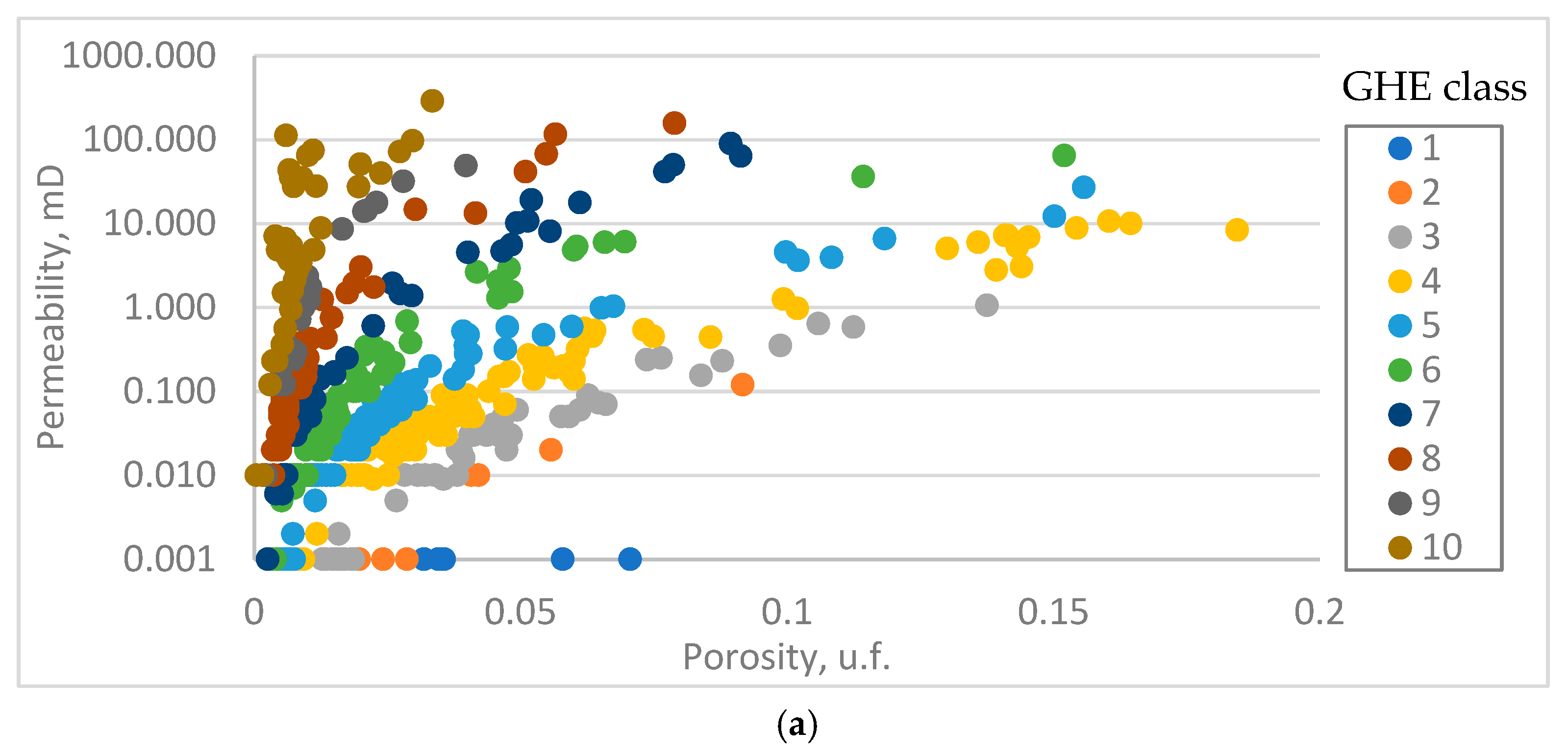
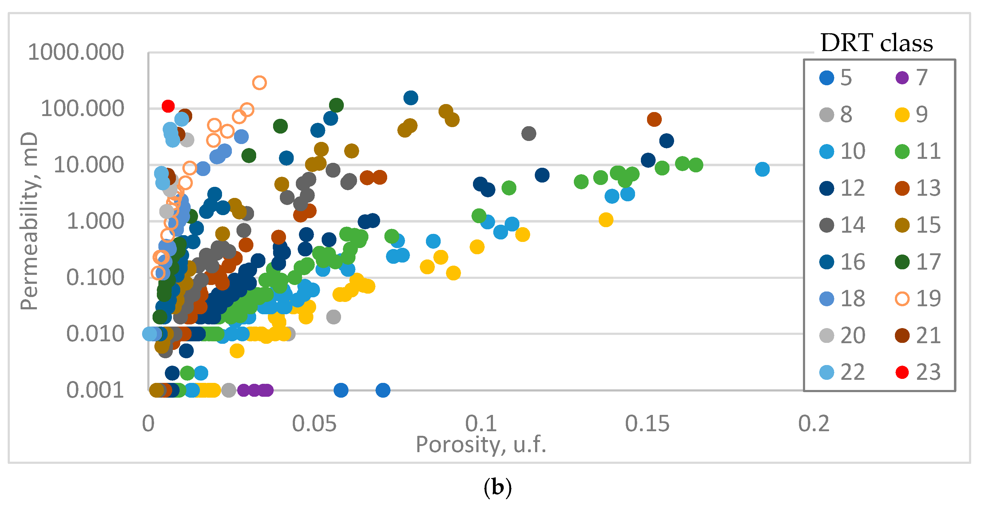
Firstly, after the FZI calculation, rock typing was carried out using the Global Hydraulic Unit (GHE) and Discrete Rock Typing (DRT) methods. Figure 5 compares the GHE and DRT classifications using the Alpha field as an example.
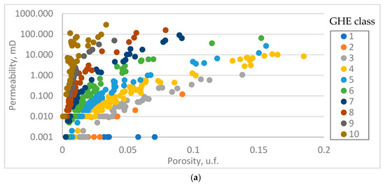
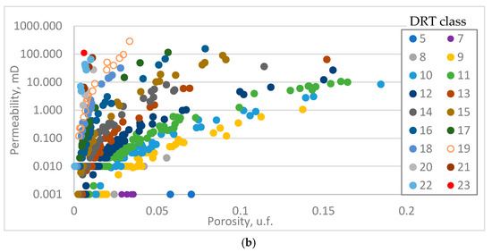
Figure 5.
Comparison of (a) GHE and (b) DRT classifications.
In the DRT discrete rock type classification, a significantly higher number of rock types is distinguished (19) compared to the GHE typing (10). This distinction results in narrower rock types, while it succeeds in increasing the coefficient of determination for certain classes. Table 1 presents a comparison of equations and coefficients of determination by type. The DRT values from 5 to 23 correspond to classes 1–19. For classes 1–3 and 19, it was impossible to build dependencies due to the small number of samples in the class.

Table 1.
Comparison of GHE and DRT classifications.
Table 1 shows an increase in the determination coefficients when using the DRT approach. Determination coefficients for all classes, except for class 18, are higher than 0.8. For class 18, the determination coefficient is 0.58; however, this type belongs to the fracture type and is characterized by a large scatter of properties, and the number of values is only six. This methodology allows us to obtain high coefficients of determination but distinguishes many classes, which will complicate the distribution of rock types in the geomodelling process.
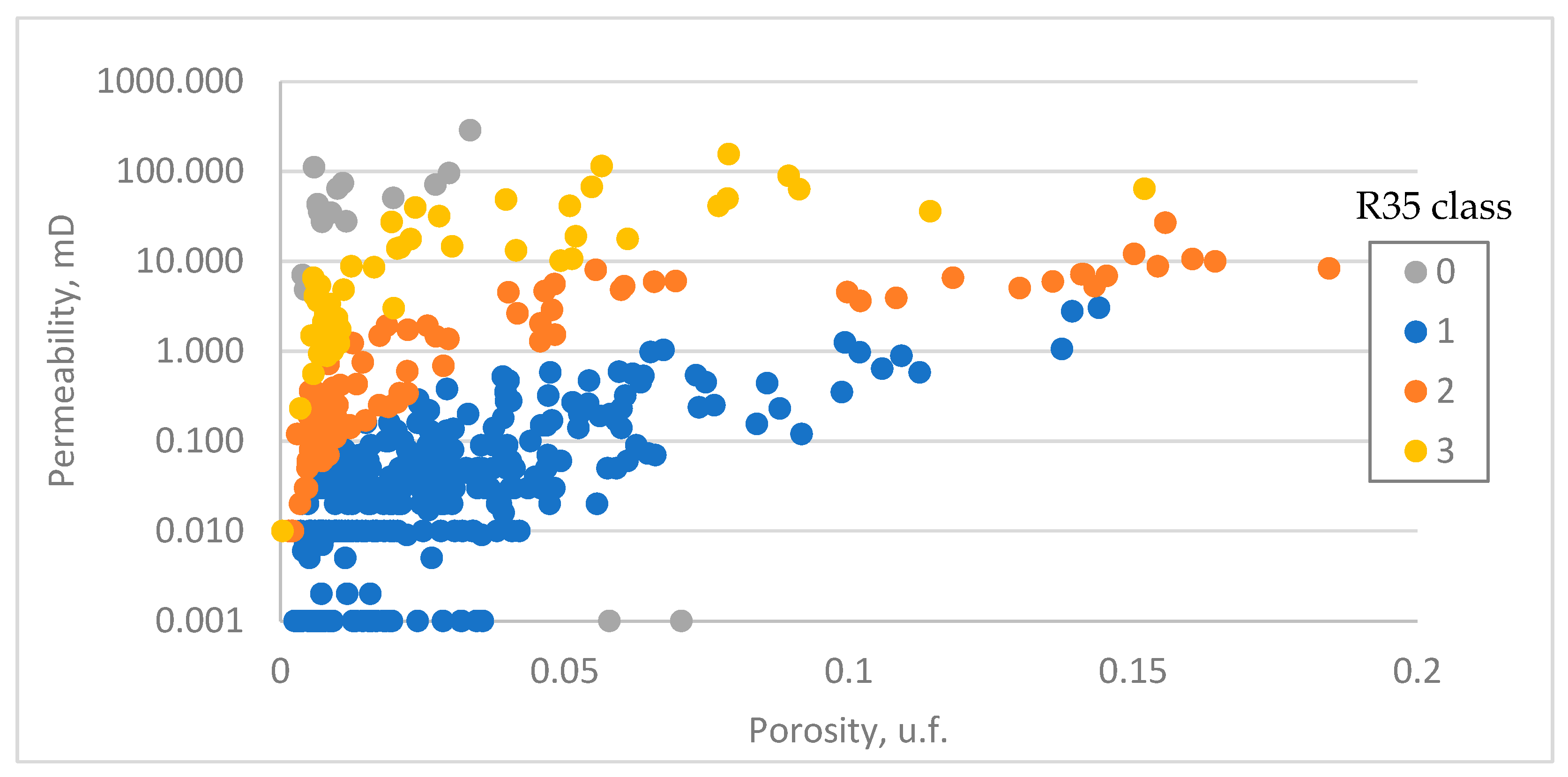
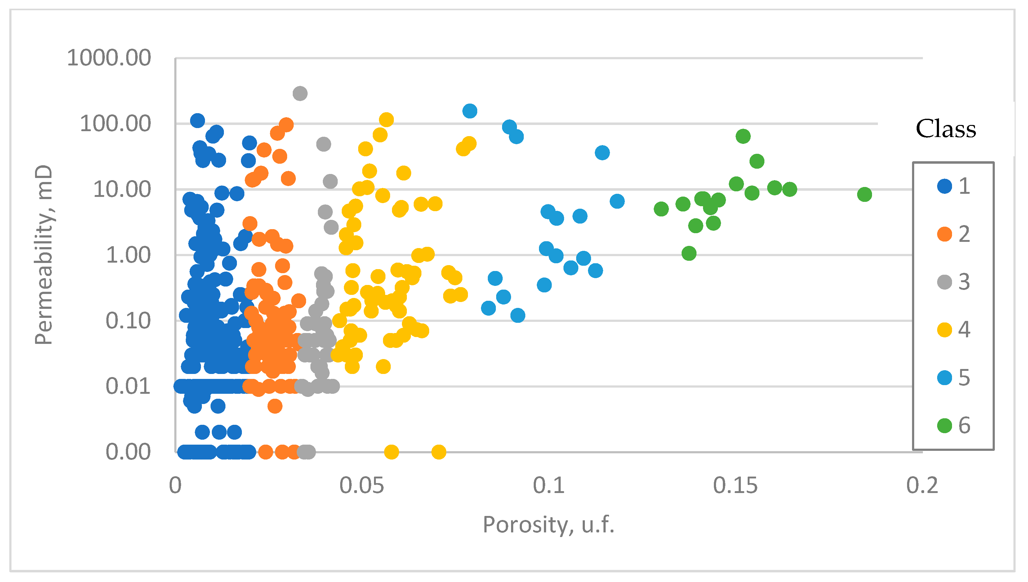
In the next stage of the work, the pore channel radius corresponding to 35% saturation of the pore volume with a nonwetting phase was calculated using the Winland equation. The reservoir was typified according to the method classification [16], i.e., four classes were identified;
- Class 1—micropores (0.1 µm < R35 < 0.5 µm);
- Class 2—mesopores (0.5 µm < R35 < 2 µm);
- Class 3—macropores (2 µm < R35 < 10 µm);
- Class 0—caverns (>10 µm).
Figure 6 shows the results of rock typing using this method.
Figure 6.
Classification by pore channel radius. The Alpha field.
Apparently, distinguishing only four classes does not provide reliable reservoir typing with high coefficients of determination between parameters in each class. However, the pore channel radius parameter can be used as one of the rock typing criteria.
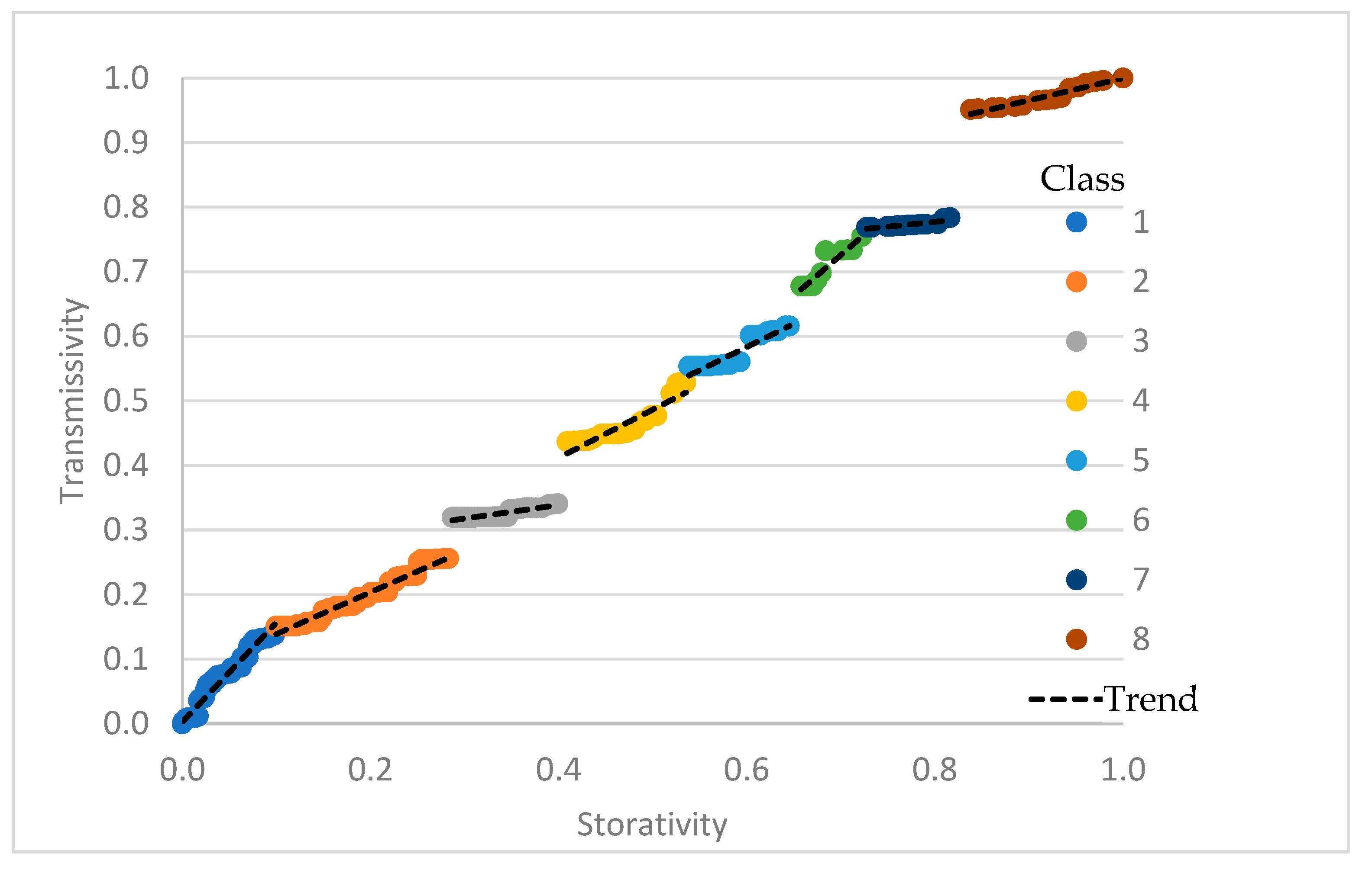
A typing exercise based on the results of the Lorenz curve is presented in Figure 7.
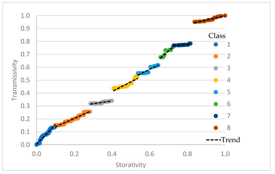
Figure 7.
Building a Lorenz curve for sample typing. The Alpha field.
Describing this plot (Figure 7), one can conventionally identify zones of sharp changes in the trends of the curve of accumulated values. These changes are characterized by a change in rock type.
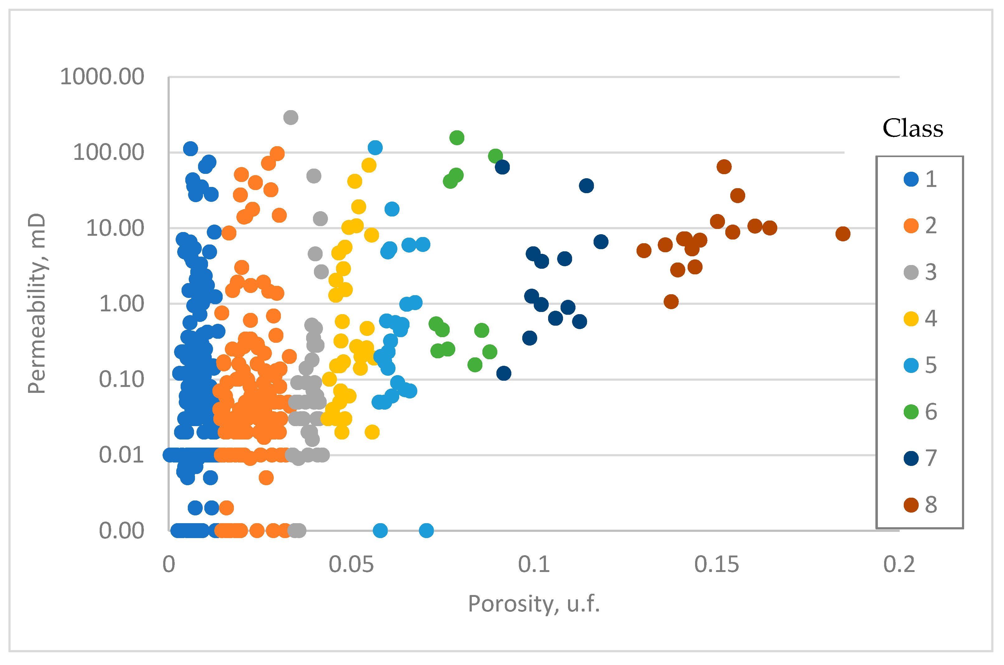
Thus, the Lorenz curve method of rock typing distinguishes eight classes in petrophysical dependency (Figure 8).
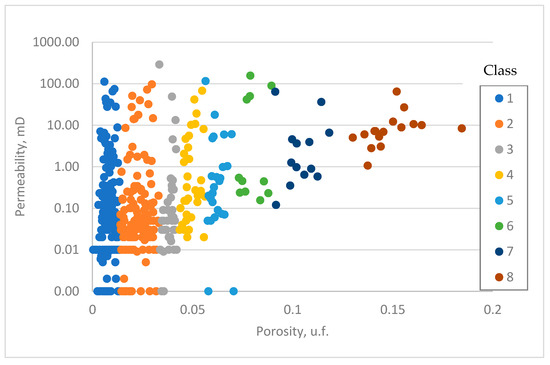
Figure 8.
Lorenz curve typing of reservoirs. The Alpha field.
Figure 8 identifies eight rock types, but the prevailing parameter in this classification is rock porosity. It can be seen that within rock types, it is not possible to obtain high values of the coefficient of determination between the parameters. Such an approach is appropriate when justifying the boundary values of porosity in modeling. Often, in order to recreate a cloud of petrophysical dependency values, the model is divided by porosity samples (bins), and the dependencies are plotted within the resulting classes. Determination coefficients in this approach remain low, but the model cubes allow to reproduction of the initial cloud of petrophysical dependence points. The extended practice is to distinguish porosity intervals based on arbitrary criteria, and this approach allows this to be conducted in a justified manner.
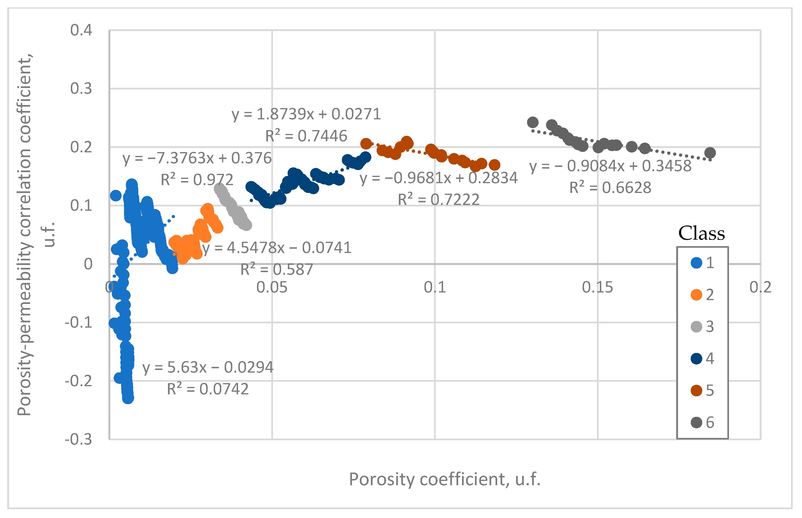
The next applied approach is also based on the analysis of accumulated values of the correlation coefficient between porosity and permeability as porosity values increase. The typing using this methodology is shown in Figure 9.
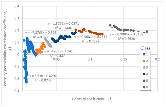
Figure 9.
Correlation coefficient between permeability and porosity versus porosity. The Alpha field.
In Figure 9, six types of rocks can be distinguished according to changes in trends. Determination coefficients were calculated for the classes, ranging from 0.07 to 0.972. The first class is characterized by a low coefficient of determination, as the relationship between permeability and porosity values is practically absent and unstable. This class can be attributed to the matrix component with the inclusion of samples with fractures and samples with practically no reservoir properties. For the second class, there is an upward trend in the correlation value between the parameters, but some samples, on the contrary, are out of the trend, probably because of the inclusion of fractures in the matrix type of the reservoir. For the third class, with increasing porosity values, there is a decreasing trend in the correlation coefficient between porosity and permeability, i.e., there are samples with fractured reservoir type—with generally low porosity, a number of samples have high permeability. The next class, four, is characterized by a general growth trend in the porosity–permeability relationship. This class may be classified as a pore reservoir. The fifth class, on the contrary, manifests a general downward trend of porosity-permeability relationship, and the cavernous component can be observed. The last class also belongs to the pore-cavernous or pore-cavernous-fracture type.
The results of rock typing are shown in Figure 10.
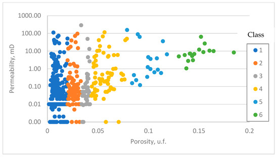
Figure 10.
Rock typing by the accumulated correlation plot. The Alpha field.
The previous approach is based on accumulated parameter values; this approach plots the division of samples into rock types predominantly by porosity. This approach can be applied to reconstruct the petrophysical dependency cloud in a geological model, but for correct rock typing, it is necessary to use the FZI parameter, which allows the correct segregation of rock types based on both porosity and permeability values. This is especially relevant when separating low-quality and fractured reservoirs. Therefore, the FZI parameter is the basis for rock typing in further study.
Previously, boundaries for rock types were calculated using the GHE and DRT methods, which provided fairly good results, but these boundaries are based on the experience of researchers and are calculated for fields of different territories. It is proposed to select boundaries for rock typing of reservoirs of the fields of the Denisovsky Depression. Machine learning methods have been used for this purpose.
The main indicators for clustering are the calculated FZI parameter and R35. Clustering was carried out for the calculated FZI values, as well as jointly for FZI and R35. The k-means and EM methods were used for clustering.
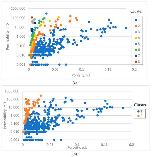
Figure 11.
Comparison of: (a) k-means; (b) EM rock typing by FZI parameter.
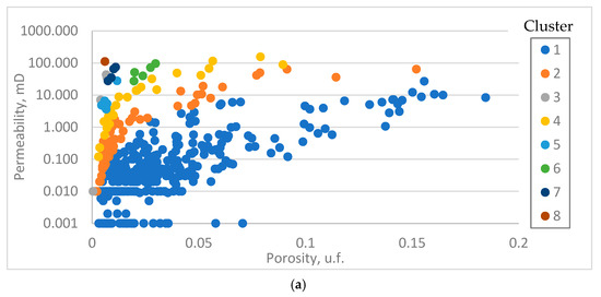
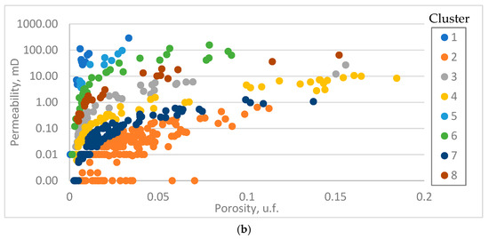
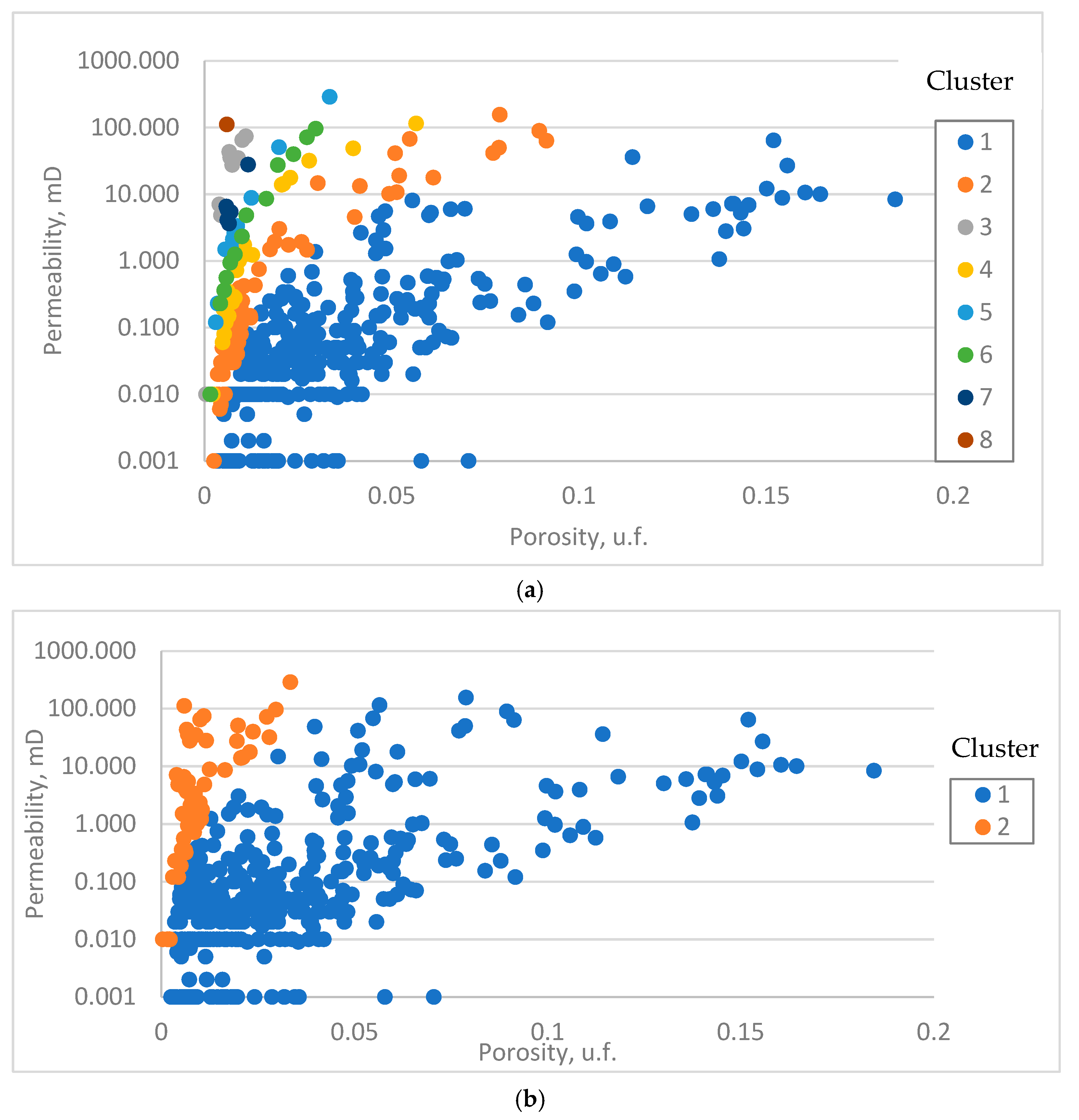
Figure 12.
Comparison of: (a) k-means; (b) EM rock typing by FZI and R35 parameters.
Figure 11 shows that clustering by the FZI parameter does not reliably separate samples into rock types. The first class has a dominant influence on clustering. Therefore, it was decided to add the pore channel radius parameter calculated earlier to improve clustering quality (Figure 12).
With the R35 parameter added for the k-means method, there is an improvement in the classification of rock types, but the first class remains predominant. The EM algorithm allowed the samples to be divided into almost equal parts, of course, with a preference for the first class, but this was not critical. Therefore, it is proposed that the EM algorithm and the distinguished criteria for FZI and R35 typing be used in further analysis. In the next step, calculations with n = 10 and n = 12 were performed to select the optimal number of clusters. The results of the classifications comparison are shown in Figure 13.

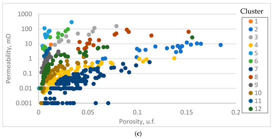
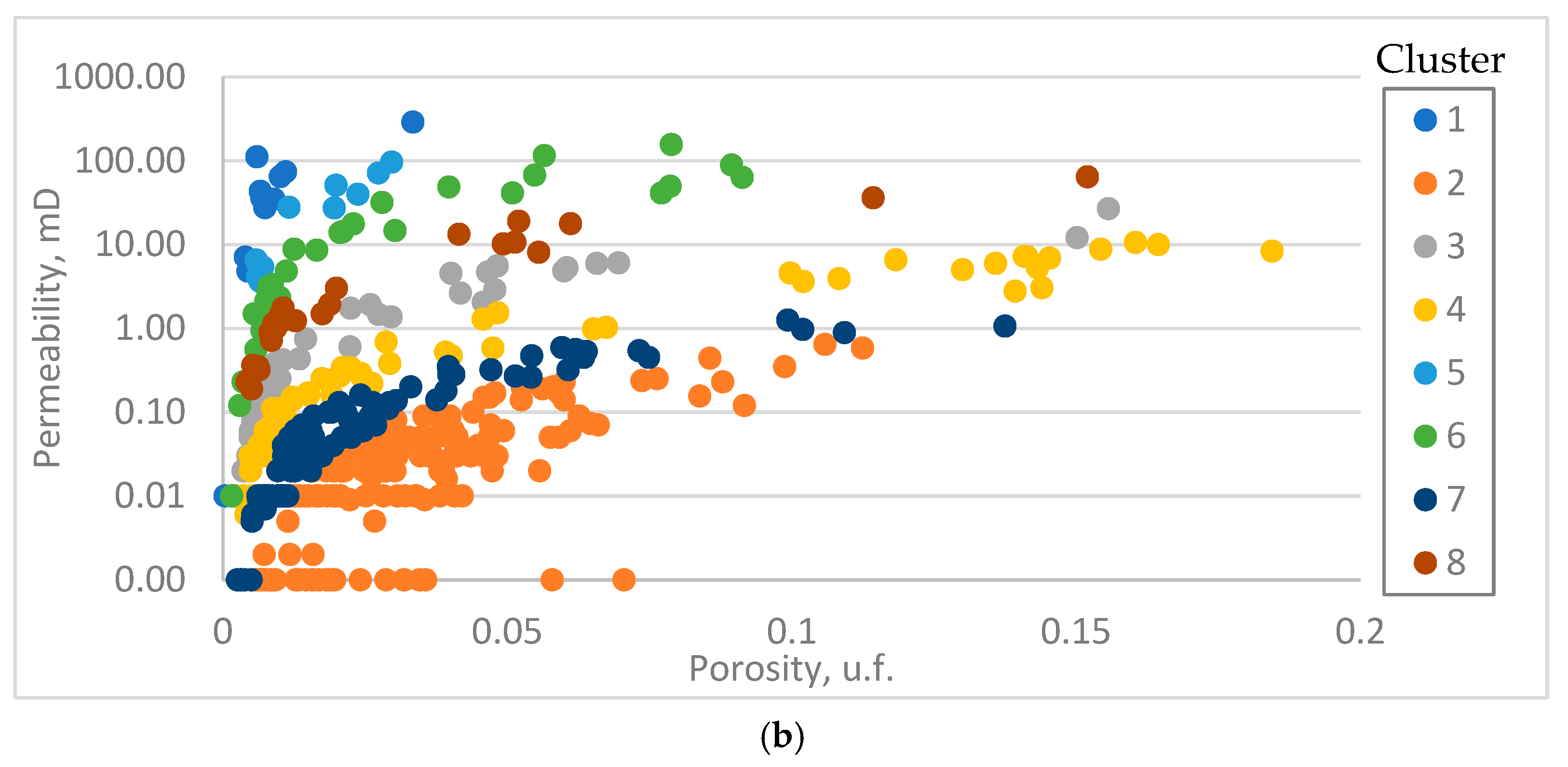
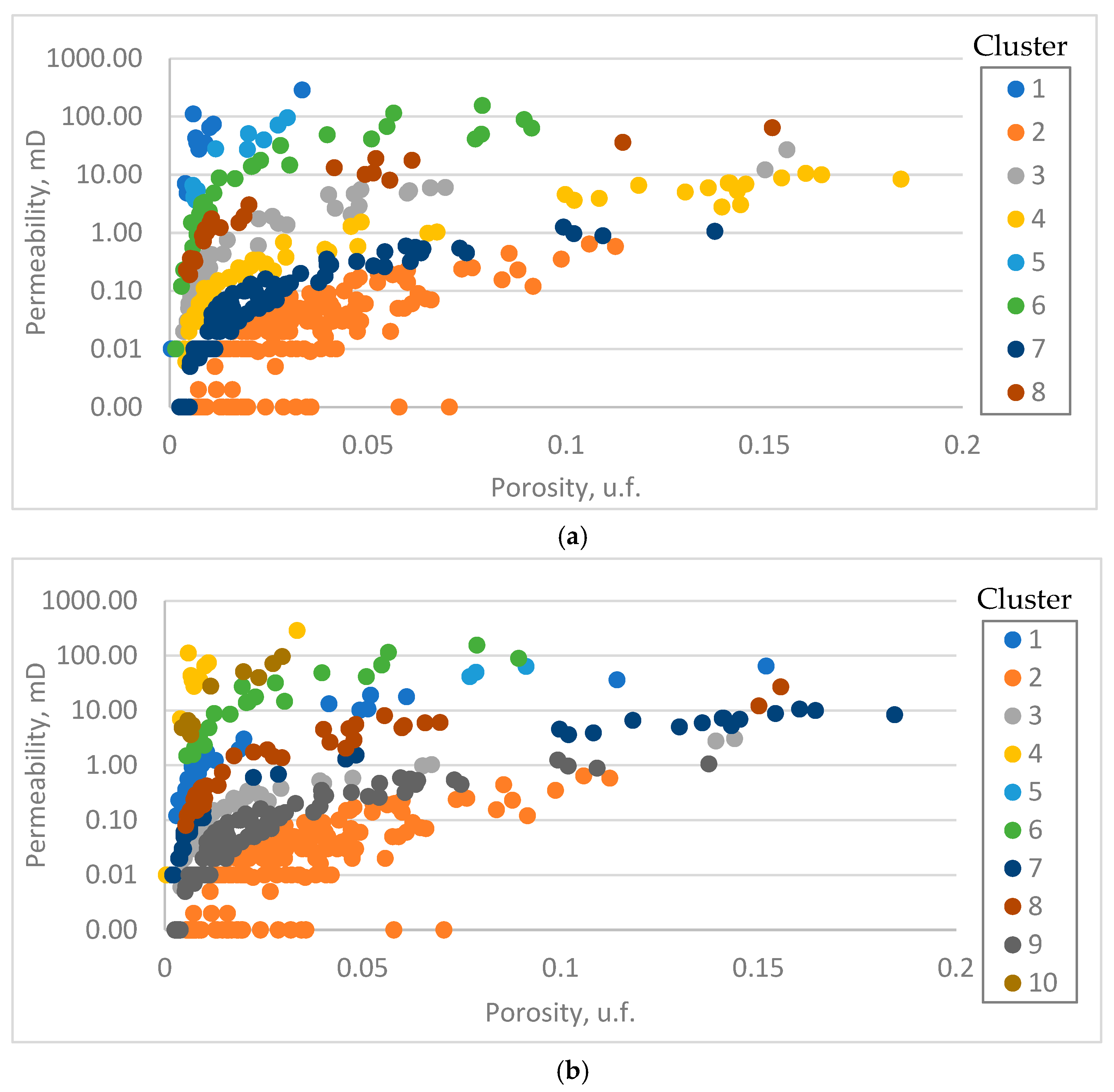
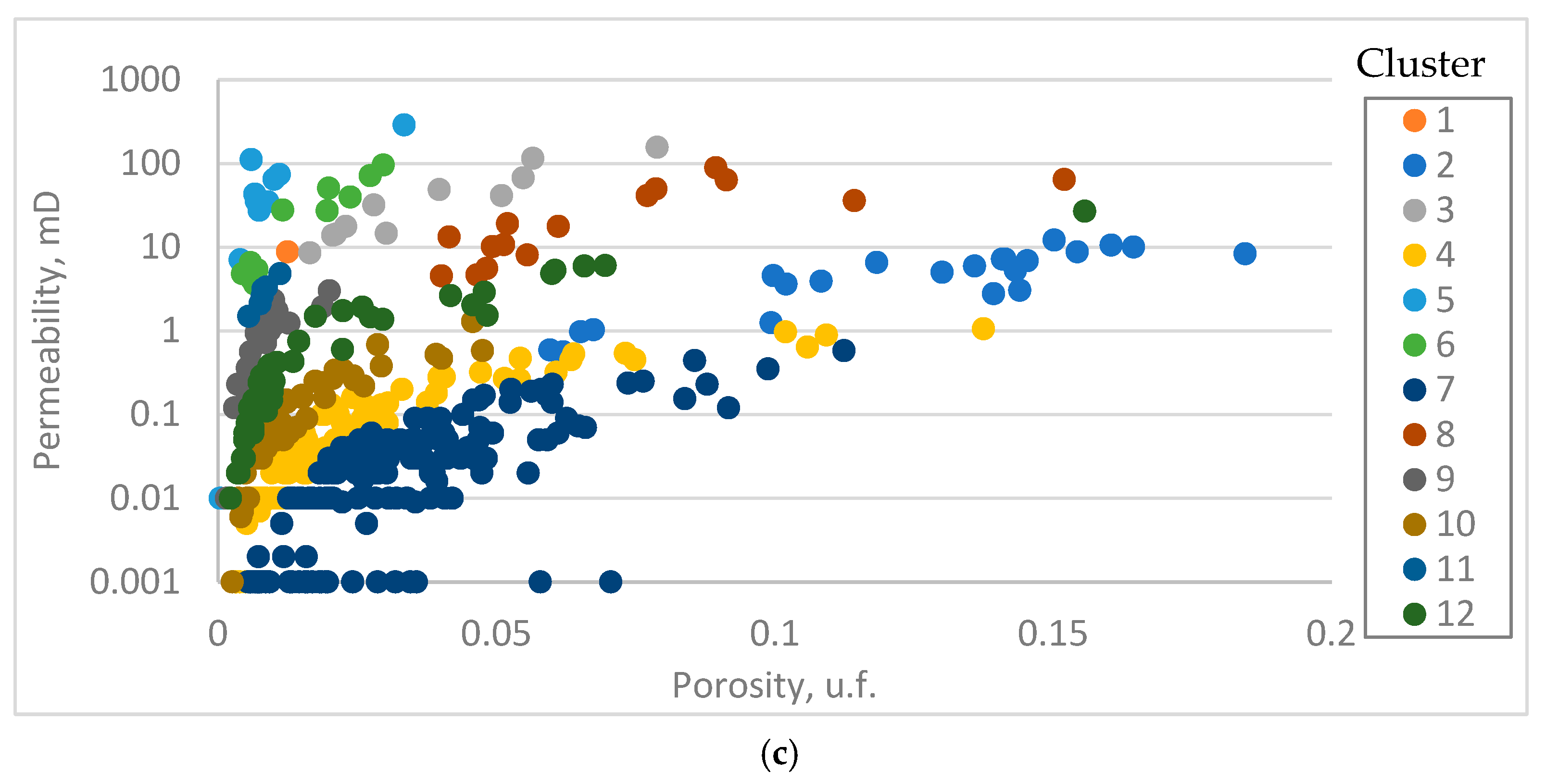
Figure 13.
Comparison of rock typing by EM method to select the number of clusters (rock types). Number of clusters: (a) 8; (b) 10; (c) 12.
As a result, clustering models have been derived that allow rock types to be distinguished with a high degree of confidence, as confirmed by the coefficients of determination between permeability and porosity parameters within classes.
The comparison of the coefficients of determination for different numbers of clusters is presented in Table 2.
Table 2.
Comparison of determination coefficients for different numbers of clusters. EM algorithm.
From Table 2, it can be concluded that, in general, it was possible to improve rock typing compared to standard approaches (GHE, DRT, R35). When using the EM clustering algorithm, determination coefficients for all cases are higher than 0.57, even for classes characterizing the fractured type of reservoir. Based on the analysis of Table 2, differences in approximation formulas are observed. For calculation with the number of clusters equal to eight, all dependencies by classes are approximated linearly with high coefficients of determination. Essentially, this approach simplifies the dependencies between permeability and porosity, but in the modeling phase, it can have the effect of overestimating the permeability. Generally, exponential relationships are adopted to approximate porosity and permeability relationships.
For a calculation with the number of clusters equal to 10, only two classes stand out that need to be approximated linearly; the remaining dependencies are exponential. Importantly, the linear dependencies are obtained only for classes that are characterized by a high correlation between porosity and permeability. That is, when porosity increases, permeability values also increase. The types of reservoirs are pore and pore-cavernous. For more complex void space types, exponential relationships are used.
For calculations with the number of clusters equal to 12, the obtained coefficients of determination are lower, but nevertheless not lower than 0.57. Three classes characterizing pore, pore-cavernous, and cavernous-pore reservoir types are also distinguished, which are approximated linearly.
The rock types corresponding to the main secondary rock transformations that have influenced the change in void space structure have been identified. Rocks of rock types 4–5 are fractured, partly dolomitized; 6, 1, 5 fractured and leached, partly dolomitized; 7–8 mostly leached, partly dolomitized; rock types 3–9 are mostly porous, partly dolomitized; rock type 2 is porous, occasionally cavernous, dolomitization and partial leaching processes are present.
According to clustering algorithms implementation, two criteria for rock typing were indicated: FZI and R35. The use of these criteria combination significantly enhances the rock classification through clustering methods. Table 3 shows the comparison between all feasible rock typing methods for reservoir modeling.
Table 3.
Comparison of different rock typing methods by statistical analysis of determination coefficients.
In terms of comparison, the results indicate that the EM clustering algorithm with 10 clusters exhibits one of the highest mean and minimal values of R2, as well as the lowest variance and coefficient of variation. This suggests the least difference in R2 between rock types and enhances the reliability of predicting the correlation between porosity and permeability. It is important to mention that, for the other methods, classes with a limited number of values stand out, preventing a dependable identification of the parameter correlation. Despite the high maximum R2 values for the DRT and GHE methods, these are observed only for classes with a number of core samples less than 10 or due to the division into a large number of classes. While the DRT and GHE methods are consistent, the EM clustering algorithm is better suited to the geological settings of the Alpha oilfield.
Based on the study results, it is found that the FZI and R35 criteria, 10 clusters (classes), and the EM clustering algorithm should be used for optimal and automatic rock typing.
5. Conclusions
A review of the main rock typing methods was carried out in this research. It was found that a significantly higher number of rock types (19) is identified on the basis of classification using the DRT discrete rock types method compared to GHE typing (10). This separation makes it possible to identify narrower rock types while increasing the coefficient of determination for certain classes. The DRT method produces high determination coefficients, but many classes are distinguished, which would make it difficult to distribute rock types when averaging properties onto a model grid and upscaling it.
The pore channel radius corresponding to 35% saturation of the pore volume with the nonwetting phase (R35) was calculated. A classification based on the R35 parameter has been carried out, but the method will not produce a reliable reservoir typology with high coefficients of determination between the parameters in each class.
Typing was carried out using the method of Lorenz plots. This method does not produce high permeability-porosity correlations between the parameters within the rock types.
Rock typing has been carried out based on the calculation of the accumulated correlation coefficient. This approach can be applied to reconstruct the petrophysical dependence cloud in the geological model, but in the authors’ opinion, for the most correct rock typing, it is necessary to use the FZI parameter, which allows to distinguish rock types more correctly, especially when separating low-quality and fractured reservoirs.
By using different rock typing methods and evaluating the relationship between porosity and permeability, it was found that FZI and R35 are the necessary criteria for selecting rock types, and their combination allows for improved quality of type predictions. On the basis of these criteria, clustering was carried out using machine learning methods. The clustering based on the EM algorithm allowed us to identify 10 rock types with high coefficients of determination. The identified rock types corresponded to the main secondary rock transformations that affected the structure of the void space. Rocks of rock types 4–5 are prone to fracturing, partly dolomitized; 1, 5, 6 are fractured and leached, partly dolomitized; 7–8 are mainly leached, partly dolomitized; rock types 3, 9 are mainly pore type, partly dolomitized; rock type 2 is porous, occasionally cavernous, dolomitization and partial leaching processes are present. These rock types have been chosen as the basis for further geological and dynamic modeling.
In future research, the authors plan to use machine learning algorithms for combining core and well-logging studies to determine rock types in intervals not characterized by core sampling. This will allow rock types to be distributed in the reservoir volume in the most reliable manner for both core-sampled intervals and the rest of the section. In the intervals of rock types, it is proposed to propagate the obtained permeability–porosity relationships for permeability array modeling, taking into account the high heterogeneity of the reservoir.
Author Contributions
Conceptualization, S.K. and A.K.; methodology, S.K.; software, A.K.; validation, N.K., A.B. and O.K.; formal analysis, A.K.; investigation, A.B. and E.O.; resources, S.K.; data curation, N.K.; writing—original draft preparation, A.K.; writing—review and editing, A.B.; visualization, N.K. and E.O.; supervision, O.K.; project administration, S.K.; funding acquisition, O.K. All authors have read and agreed to the published version of the manuscript.
Funding
This study was conducted under the Russian Science Foundation grant №. 22-17-00111.
Data Availability Statement
Not applicable.
Conflicts of Interest
The authors declare no conflict of interest.
References
- Tavakoli, V. Carbonate Reservoir Heterogeneity: Overcoming the Challenges; Springer International Publishing: Tehran, Iran, 2019; pp. 1–108. [Google Scholar]
- Sharifi-Yazdi, M.; Rahimpour-Bonab, H.; Nazemi, M.; Tavakoli, V.; Gharechelou, S. Diagenetic impacts on hydraulic flow unit properties: Insight from the Jurassic carbonate Upper Arab Formation in the Persian Gulf. J. Pet. Explor. Prod. Technol. 2020, 10, 1783–1802. [Google Scholar] [CrossRef]
- Tabrizinejadas, S.; Fahs, M.; Hoteit, H.; Younes, A.; Ataie-Ashtiani, B.; Simmons, C.; Carrayrou, J. Effect of temperature on convective-reactive transport of CO2 in geological formations. Int. J. Greenh. Gas Control 2023, 128, 103944. [Google Scholar] [CrossRef]
- Al-Otaibi, M.; Abdullah, E.; Hanafy, S. Prediction of Permeability from Logging Data Using Artificial Intelligence Neural Networks. In Proceedings of the SPE Western Regional Meeting, Anchorage, AK, USA, 22–25 May 2023. [Google Scholar] [CrossRef]
- Mustafa, R.; Sameera, H. Studying the Effect of Permeability Prediction on Reservoir History Matching by Using Artificial Intelligence and Flow Zone Indicator Methods. Iraqi Geol. J. 2023, 56, 9–21. [Google Scholar] [CrossRef]
- Zolotukhin, A.B.; Gayubov, A.T. Machine learning in reservoir permeability prediction and modelling of fluid flow in porous media. IOP Conf. Ser. Mater. Sci. Eng. 2019, 700, 012023. [Google Scholar] [CrossRef]
- Efremova, E.I.; Putilov, I.S. On the question of hydraulic flow units use in terrigenous deposits taking into account facies (on the example of the Sof’inskoye field in the Perm Krai). J. Pet. Min. Eng. 2022, 22, 52–57. [Google Scholar]
- Antoniuk, V.; Bezrodna, I.; Petrokushyn, O. Multiple regressions and ann techniques to predict permeability from pore structure for terrigenous reservoirs, west-shebelynska area. Eur. Assoc. Geosci. Eng. 2019, 2019, 1–5. [Google Scholar] [CrossRef]
- Srinivasan, S.; Leung, J.Y. Petroleum Reservoir Modeling and Simulation: Geology, Geostatistics, and Performance Prediction, 1st ed.; McGraw Hill: New York, NY, USA, 2022; Available online: https://www.accessengineeringlibrary.com/content/book/9781259834295 (accessed on 1 February 2023).
- Haddad, A.; Lathion, R.; Courgeon, S.; Fabre, G.; Martinuzzi, V.; Pedraza, S.; Hauvette, L.; Games, F. Multi-Scale Karstic Reservoir Characterization: An Innovative Approach to Improve Reservoir Model Predictions and Decision Making. In Proceedings of the International Petroleum Technology Conference, Riyadh, Saudi Arabia, 21–23 February 2022. [Google Scholar] [CrossRef]
- Mulyanto, B.; Dewanto, O.; Yuliani, A.; Yogi, A.; Wibowo, R. Porosity and permeability prediction using pore geometry structure method on tight carbonate reservoir Porosity and permeability prediction using pore geometry structure method on tight carbonate reservoir. In Proceedings of the 9th International Conference on Theoretical and Applied Physics (ICTAP), Bandar Lampung, Indonesia, 15 July 2020. [Google Scholar] [CrossRef]
- Krivoshchekov, S.; Kochnev, A.; Kozyrev, N.; Ozhgibesov, E. Factoring Permeability Anisotropy in Complex Carbonate Reservoirs in Selecting an Optimum Field Development Strategy. Energies 2022, 15, 8866. [Google Scholar] [CrossRef]
- Lathion, R.; Courgeon, S.; Martinuzzi, V.; Fabre, G.; Haddad, A.; Games, F. Identification and integrated characterization of large-scale karstic network: Critical impact on reservoir understanding and modeling. In Proceedings of the 8ème Congrès Français de Sédimentologie—ASF 2022, Brest, Belarus, 28–30 September 2022. [Google Scholar]
- Shishaev, G.; Demyanov, V.; Arnold, D.; Vygon, R. History Matching and Uncertainty Quantification of Reservoir Performance with Generative Deep Learning and Graph Convolutions. In Proceedings of the International Petroleum Technology Conference, Riyadh, Saudi Arabia, 21–23 February 2022. [Google Scholar] [CrossRef]
- Robail, F.; Sanyal, S.; Azudin, A.; Koh, K.; Nizar, F.; Rosli, U. Machine Learning for Facies Distribution of Large Carbonate Reservoir Models—A Case Study. In Proceedings of the International Petroleum Technology Conference, Bangkok, Thailand, 1–3 March 2023. [Google Scholar] [CrossRef]
- Elarouci, F.; Maalouf, C.; Espinoza, I.; Al-jaberi, S.; Amer, M.; Smith, S.; Jalalh, A. Integrated Reservoir Characterization to Approach the Carbonate Permeability Distribution Challenges: Case Study from Offshore Abu Dhabi. In Proceedings of the Abu Dhabi International Petroleum Exhibition & Conference, Abu Dhabi, United Arab Emirates, 7–10 November 2016. [Google Scholar] [CrossRef]
- Albreiki, M.; Geiger, S.; Corbett, P. Impact of modelling decisions and rock typing schemes on oil in place estimates in a giant carbonate reservoir in the Middle East. Pet. Geosci. 2021, 28, 1–21. [Google Scholar] [CrossRef]
- Palabiran, M.; Sesilia, N.; Akbar, M.N.A. An Analysis of Rock Typing Methods in Carbonate Rocks For Better Carbonate Reservoir Characterization: A Case Study of Minahaki Carbonate Formation, Banggai Sula Basin, Central Sulawesi. In Proceedings of the 41th Scientific Annual Meeting of Indonesian Association of Geophysicists, Lampung, Indonesian, 26–29 September 2016. [Google Scholar]
- Archie, G.E. Classification of Carbonate Reservoir Rocks and Petrophysical Considerations. AAPG Bull. 1952, 36, 278–298. [Google Scholar] [CrossRef]
- Raznicyn, A.; Putilov, I. Development of a Methodological Approach to Identifying Petrophysical Types of Complicated Carbonate Rocks According to Laboratory Core Studies. Perm J. Pet. Min. Eng. 2021, 21, 109–116. [Google Scholar] [CrossRef]
- Ghanbarian, B.; Lake, L.; Sahimi, M. Insights Into Rock Typing: A Critical Study. SPE J. 2018, 24, 230–242. [Google Scholar] [CrossRef]
- Ellabad, Y.; Corbett, P.W.M.; Straub, R. Hydraulic Units approach conditioned by well testing for better permeability modeling in a North African Oil Field. In Proceedings of the 2001 International Symposium of the Society of Core Analysts, Edinburgh, UK, 17–19 September 2001. [Google Scholar]
- Lazim, S.A.; Hamd-Allah, S.M.; Jawad, A. Permeability Estimation for Carbonate Reservoir (Case Study/South Iraqi Field). Iraqi J. Chem. Pet. Eng. 2018, 19, 41–45. [Google Scholar] [CrossRef]
- El-Sawy, M.Z.; Abuhagaza, A.A.; Nabawy, B.; Lashin, A. Rock typing and hydraulic flow units as a successful tool for reservoir characterization of Bentiu-Abu Gabra sequence, Muglad basin, southwest Sudan. J. Afr. Earth Sci. 2020, 171, 103961. [Google Scholar] [CrossRef]
- Nabawy, B.; Rashed, M.; Mansour, A.; Afifi, W. Petrophysical and microfacies analysis as a tool for reservoir rock typing and modeling: Rudeis Formation, off-shore October Oil Field, Sinai. Mar. Pet. Geol. 2018, 97, 260–276. [Google Scholar] [CrossRef]
- Irawan, D.; Wihdany, F.I.; Idea, K. Permeability Anisotropy Effect in Reservoir Characterization: New Rock Typing Approach. In Proceedings of the Forty-Third Annual Convention & Exhibition, Jakarta, Indonesia, 4–6 September 2019. [Google Scholar]
- Kolodzie, S. Analysis of pore throat size and use of the Waxman–Smits equation to determine OOIP in Spindle Field, Colorado. In Proceedings of the SPE Annual Technical Conference and Exhibition, Dallas, TX, USA, 21 September 1980. [Google Scholar] [CrossRef]
- Pittman, E.D. Relationship of porosity and permeability to various parameters derived from mercury injection-capillary pressure curves for sandstone. Am. Assoc. Pet. Geol. Bull. 1992, 76, 191–198. [Google Scholar] [CrossRef]
- Sousa, A.M.; Ines, N.; Bizarro, P.; Ribeiro, M.T. Improving Carbonate Reservoir Characterization and Modelling through the Definition of Reservoir Rock Types by Integrating Depositional and Diagenetic Trends. In Proceedings of the Abu Dhabi International Petroleum Exhibition and Conference, Abu Dhabi, United Arab Emirates, 10–13 November 2014. [Google Scholar] [CrossRef]
- Permadi, P.; Susilo, A. Permeability Prediction and Characteristics of Pore Structure and Geometry as Inferred from Core Data. In Proceedings of the 2009 SPE/EAGE Reservoir Characterization and Simulation Conference, Abu Dhabi, United Arab Emirates, 19–21 October 2009. [Google Scholar] [CrossRef]
- Choquette, P.W.; Pray, L.C. Geologic Nomenclature and Classification of Porosity in Sedimentary Carbonates. Am. Assoc. Pet. Geol. Bull. 1970, 54, 207–250. [Google Scholar] [CrossRef]
- Dunham, R.J. Classification of Carbonate Rocks According to Depositional Texture. In Classification of Carbonate Rocks—A Symposium; The American Association of Petroleum Geologists: Tulsa, OK, USA, 1962; pp. 108–121. [Google Scholar]
- Repina, V.A.; Galkin, V.I.; Galkin, S.V. Complex petrophysical correction in the adaptation of geological hydrodynamic models (on the example of Visean pool of Gondyrev oil field). J. Min. Inst. 2018, 231, 268–274. [Google Scholar] [CrossRef]
- Galkin, V.I.; Ponomareva, I.N.; Repina, V.A. Study of the process of oil recovery in reservoirs of various types of voids using multivariate statistical analysis. Bull. Perm Natl. Res. Polytech. Univ. Geol. Oil Gas Eng. Min. 2016, 15, 145–154. [Google Scholar]
- Putilov, I.; Kozyrev, N.; Demyanov, V.; Krivoshchekov, S.; Kochnev, A. Factoring in Scale Effect of Core Permeability at Reservoir Simulation Modeling. SPE J. 2022, 27, 1930–1942. [Google Scholar] [CrossRef]
- Galvao, P.; Halihan, T.; Hirata, R. The karst permeability scale effect of Sete Lagoas, MG, Brazil. J. Hydrol. 2016, 532, 149–162. [Google Scholar] [CrossRef]
- Corbett, P.W.M.; Potter, D.K. Petrotyping: A basemap and atlas for navigating through permeability and porosity data for reservoir comparison and permeability prediction. In Proceedings of the International Symposium of the Society of Core Analysts, Abu Dhabi, United Arab Emirates, 5–9 September 2004. [Google Scholar]
- Garrouch, A.A.; Al-Sultan, A.A. Exploring the link between the flow zone indicator and key open-hole log measurements: An application of dimensional analysis. Pet. Geosci. 2019, 25, 219–234. [Google Scholar] [CrossRef]
- Lake, L.; Jensen, J. A review of heterogeneity measures used in Reservoir Characterisation. In Situ 1991, 15, 409–440. [Google Scholar]
- Gunter, G.W.; Finneran, J.M.; Hartmann, D.J.; Miller, J.D. Early Determination of Reservoir Flow Units Using an Integrated Petrophysical Method. In Proceedings of the SPE Annual Technical Conference and Exhibition, San Antonio, TX, USA, 5 October 1997. [Google Scholar] [CrossRef]
- Korablev, N.M.; Fomichev, A.A. K-means data clustering using artificial immune systems. Bionics Intell. Sci. Mag. 2011, 3, 102–106. [Google Scholar]
- Mirkin, B.G. Clustering for Data Mining. A Data recovery Approach; Chapman and Hall/CRC: New York, NY, USA, 2005; pp. 269–296. [Google Scholar] [CrossRef]
- Bradley, P.S.; Fayyad, U.M. Refining Initial Points for K-Means Clustering. In Proceedings of the International Conference on Machine Learning, San Francisco, CA, USA, 24–27 July 1998. [Google Scholar]
- Cherezov, D.S.; Tukachev, N.A. Classification and clasterization base methods review. Bull. Voronezh State Univ. Ser. Syst. Anal. Inf. Technol. 2009, 2, 25–29. [Google Scholar]


Disclaimer/Publisher’s Note: The statements, opinions and data contained in all publications are solely those of the individual author(s) and contributor(s) and not of MDPI and/or the editor(s). MDPI and/or the editor(s) disclaim responsibility for any injury to people or property resulting from any ideas, methods, instructions or products referred to in the content. |
© 2023 by the authors. Licensee MDPI, Basel, Switzerland. This article is an open access article distributed under the terms and conditions of the Creative Commons Attribution (CC BY) license (https://creativecommons.org/licenses/by/4.0/).