Abstract
Carbon reduction programs are being introduced for carbon neutrality and energy transition to clean energy sources in various sectors, such as energy, buildings, transportation, and agriculture. In the residential electricity energy of the energy sector, the time-of-use (TOU) rate plan, which employs dynamic rates depending on energy usage times based on the advanced metering infrastructure (AMI), is being implemented for efficient electricity energy consumption. For broad expansion of the TOU rate plan, customers need information about its benefits, such as potential savings on electricity bills. In this paper, we first analyze the statistical characteristics of electricity energy usage using the metering data collected from 10 apartment complexes through AMI and develop a model to calculate the electricity bill savings. We next introduce examples of major home appliances, of which usage times can be shifted, and offer projected bill savings from the developed model. We analyze the examples from both the perspectives of households and apartment complexes. The information from this analysis is helpful in practically investigating customers’ willingness to shift the usage time for a successful implementation of the demand response program.
1. Introduction
The major countries around the world have set a goal of achieving carbon neutrality by 2050 in order to respond to global climate change. Each country has presented detailed action plans in various fields, such as energy, buildings, transportation, and agriculture, to achieve the carbon neutrality goal. Demand for electrical energy is expected to grow significantly because electricity-based solutions will replace the vehicles and heating systems in the process of achieving the carbon neutral goal. It is necessary to pay attention to carbon neutrality and energy transition especially in the residential sector, which accounts for a substantial portion of automobile and heating demand. It is known that the share of electrical energy in the residential sector accounts for about 30–40% of the total electrical energy consumption [1,2,3] and is expected to increase further in the process of achieving the carbon neutrality goal.
On the other hand, flexibility in electrical energy demand is necessary to mitigate the variability of renewable energy required for the carbon neutrality [4,5,6]. The demand flexibility can be defined by the following three variables: the amount of load that can be moved, the time period that can be used by moving, and the maximum time that such movement is allowed [7]. In addition to these quantitative variables, qualitative variables of electricity consumers are also important. The qualitative variables include energy usage habits of individuals who consume electricity, degree of discomfort, and sensitivity to electricity rates [8,9,10,11]. There is a demand response (DR) program as a way to secure the flexibility of electrical energy demand in the residential sector. DR programs for electrical energy aim to secure a balance between demand and supply by reducing or increasing the demand for electricity usage in a specific time period. These DR programs are designed on a price-based or incentive-based scheme, and customer responsiveness varies according to price signals or incentive levels. The DR program can contribute to the balancing of the power system by inducing changes in customers’ electricity usage patterns according to electricity rates for specific seasons, days, and time slots [12].
The time-of-use (TOU) rate system is known as a representative DR electricity rate system. Therefore, it is important to effectively design a TOU rate system so that the response characteristics of the customers’ electricity usage pattern can contribute to the flexible operation of the power system [8,9]. Because the suitable electricity rates for customers can be dependent on the lifestyles of electricity customers, types of home appliances, unit price of electricity, etc., electric power companies should inform customers of the advantages and disadvantages of choosing an electricity rate system by considering the customers’ power usage information. In the case of certain TOU rate systems, customers can save electricity bills even though they maintain their current electricity usage patterns. When electricity bills are reduced without the customer’s efforts to change their power usage patterns, we call these customers structural winners [13]. In order to mitigate the presence of such structural winners, power companies should design TOU rate systems so that electricity bill savings can be given when customers change their existing load usage patterns and shift load usage hours to non-demand hours. Note that most of the studies on the DR effect of dynamic rate plans, such as TOU, are based on load management methods for home appliances in a specific household. Yu et al. [14] performed an optimization scheme in usage of home appliances, and Zhang et al. [15] conducted a study on the integrated DR potential and characteristics through scheduling of home appliances for multiple households connected to a specific distribution line. Chung et al. [16] comparatively analyzed the current progressive rate plan and a dynamic rate plan of TOU. They next proposed several prediction methods for households to provide information on selecting the rate plan based on machine learning. When a customer switches to a new electricity rate plan, it is desirable for the utility to provide the customer with information about potential electricity bill savings.
In this paper, we first analyze the statistical characteristics of customers’ electricity usage and their corresponding electricity bills under the TOU rate plan by investigating the electrical load profiles (LPs), which are collected for one year from the smart meters and advanced metering infrastructure (AMI) of certain residential customers [16,17]. For a given customer group, we propose a model for monthly electricity usage and peak-hour usage ratio of households based on a Gaussian distribution and then derive an equation that yields an average of monthly electricity bills under the TOU rate plan. We next introduce examples of major home appliances that can shift their demands by using the equation. Here, the effect analysis is concerned with the amount of load shifting and whether or not the electrical bill increases or decreases according to the load shifting.
The paper is organized in the following way. In Section 2, we analyze the statistical characteristics of monthly usage and the peak-hour usage ratio of households distribution characteristics for the metering data collected from a total of 11,522 households in 10 apartment complexes, where each household has three to four rooms and two bathrooms. We also derive the bill savings from a statistical characteristic formula for a given TOU rate plan. In Section 3, we investigate the power consumptions according to the usage methods for washing machines and clothes dryers, which are representative home appliances that consume large amounts of electrical energy, and analyze the effect of shifting to other demand time zones. In the last section, we conclude the paper.
2. Analysis of Electricity Usage, Peak-Hour Usage Ratio, and TOU Rate Plan
In this section, a mathematical model for electricity bills under a TOU rate plan is developed using the electricity usage and peak-hour usage ratio obtained from actual households where people reside, through AMI. To develop a model for the average electricity bills for each household when applying the TOU rate plan, we find an approximate distribution of monthly electricity usage and the peak-hour usage ratio for households, as well as to analyze the correlation between these two values. Assuming an approximate Gaussian distribution based on observations from Q-Q plots, skewness, and kurtosis, along with the assumption of uncorrelatedness, we formulate a model for the average household bills. The model is validated through a comparison between actual and model-predicted values. Note that this study does not focus on the rigorous analysis and development of the distribution itself for monthly electricity usage and peak-hour usage ratio through the use of various statistical tests.
The TOU rate plan involves different electric rates based on the season and time of electricity use. Table 1 presents the monthly TOU rates for residential use in the Republic of Korea [16]. The rates are higher during the peak hours compared to off-peak hours, and the rates for the summer/winter case are higher than those for the other case. Additionally, a basic rate is applied to each household every month. To implement the TOU rate plan, it is necessary to collect both the time of electrical energy usage and the corresponding energy usage amount. The LP metering by AMI offers the electrical usage data along with time information at 15-minute intervals, enabling the application of the TOU rate plan.

Table 1.
Monthly TOU rate for residential use (KRW 1000 corresponds to USD 0.769 as of July 2023).
The electricity usage data of 11,522 households in 10 apartment complexes are collected hourly through AMI. The data are used to investigate the correlation between the electricity usage and the peak-hour usage ratio. Table 2 shows a summary of the apartment complexes and the number of households where data were collected.
Table 2.
Summary of the apartment complexes.
2.1. Analysis of Monthly Electricity Usage of Households
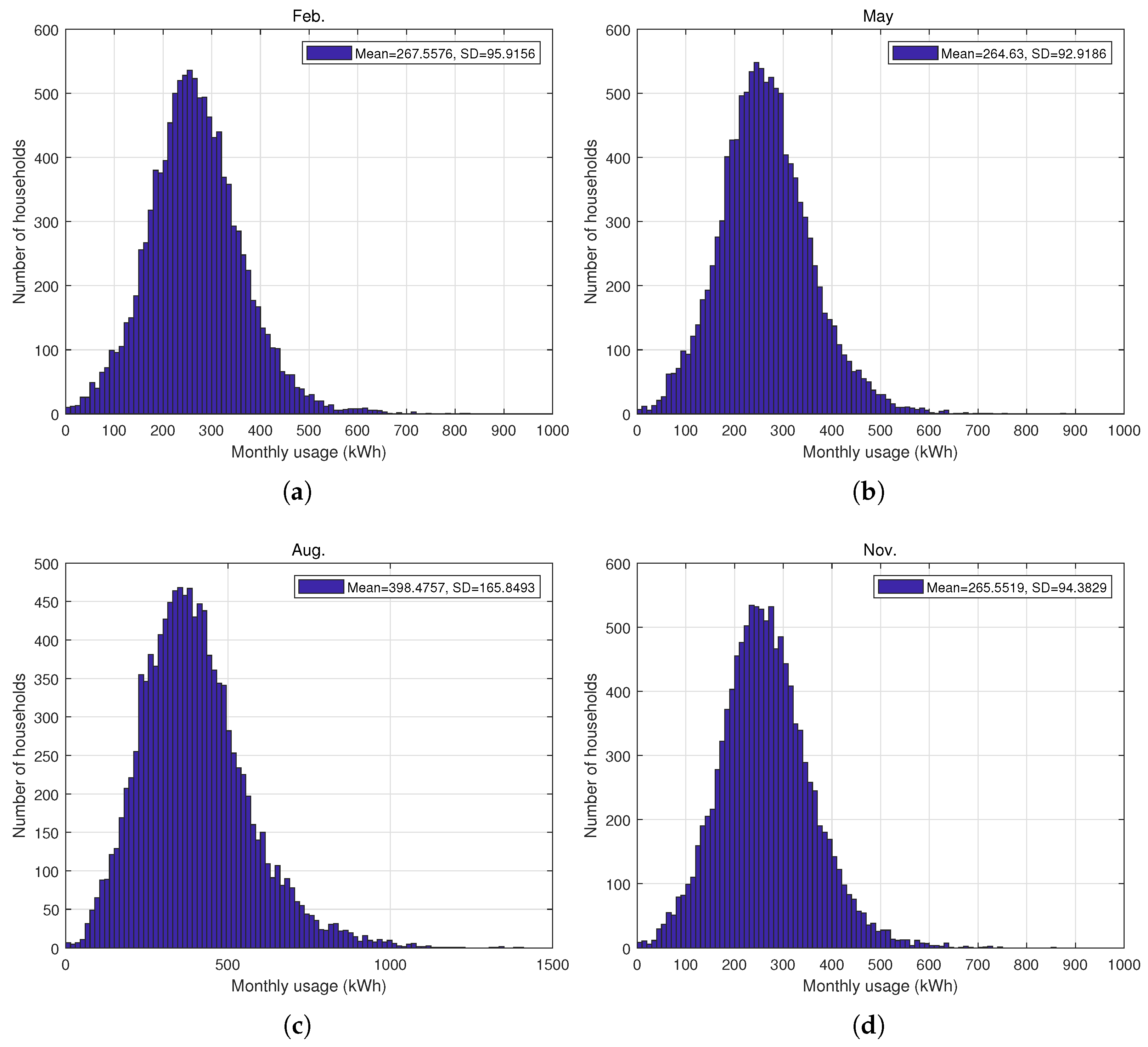
In this subsection, we determine an approximate distribution of the electricity usage of households. Using the collected electricity usage data for households, histograms are obtained for each month. All the histograms for the months exhibit a similar shape, except for that for August. As representative examples, the histograms for the months of February, May, August, and November are shown in Figure 1.

Figure 1.
Histograms of monthly electricity usage. (a) February. (b) May. (c) August. (d) November.
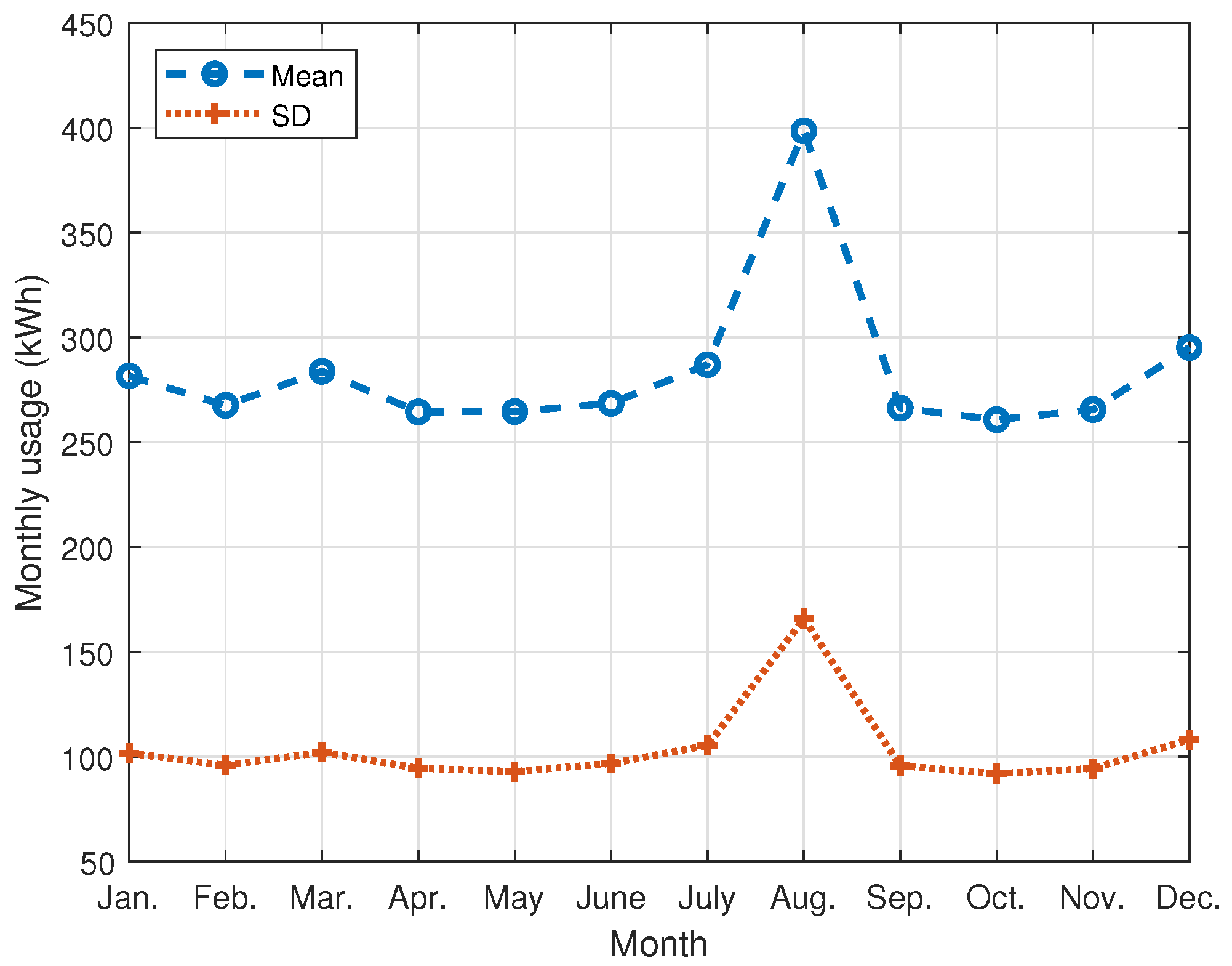
The mean and standard deviation of monthly electricity usage for households are shown in Figure 2. From the results, it is observed that except for August, there is little difference in mean and standard deviation of monthly electricity usage for households.

Figure 2.
Mean and standard deviation of monthly electricity usage for household.
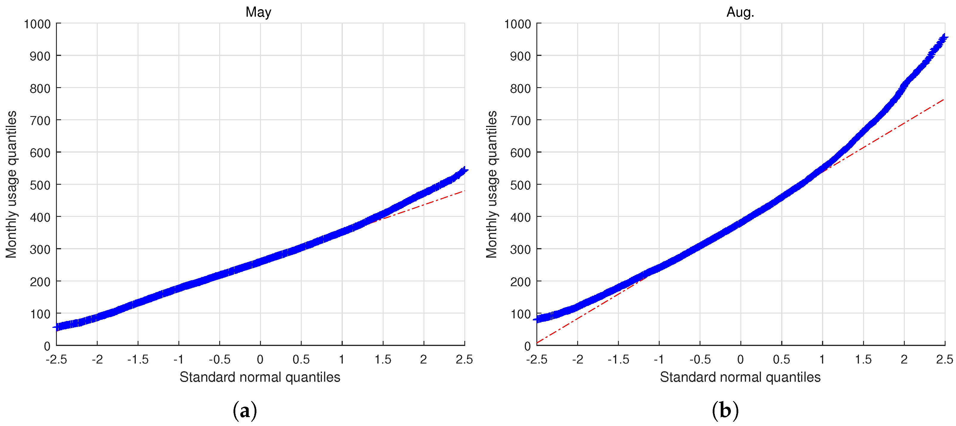
On the other hand, from Figure 1, it is observed that the histogram of electricity usage bears a resemblance to a bell-shaped Gaussian distribution, centered around the mean value. To further explore the similarity between the distribution of monthly electricity usage and a Gaussian distribution, a normal quantile-quantile (Q-Q) plot is obtained and presented in Figure 3. The normal Q-Q plot allows for a more detailed examination of the resemblance between the observed data and a theoretical Gaussian distribution by comparing their quantiles [18]. The months of June, July, August, and September exhibit similar patterns, with August being used as a representative example in Figure 3. Similarly, the remaining months exhibit similar patterns, with May being used as a representative example.
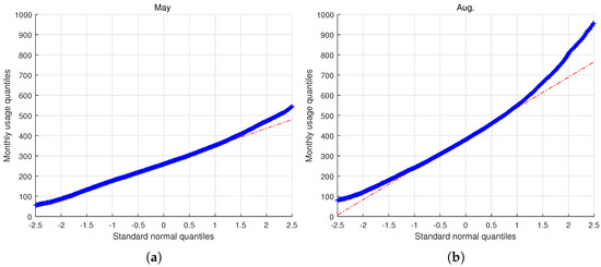
Figure 3.
Normal Q-Q plot of monthly electricity usage. (a) May. (b) August.
In Figure 3, each value on the horizontal axis corresponds to a specific quantile of the standard Gaussian distribution. Likewise, each value on the vertical axis corresponds to a specific quantile of the monthly electricity usage. The blue ‘+’ markers on the graph indicate the points where the horizontal and vertical values have the same quantile. The red dotted line in the graph represents the values that would be expected if the data followed a perfect Gaussian distribution. The closer the trace of the collected values marked by blue ‘+’ is to this red dotted line, the closer the distribution of monthly electricity usage is to a Gaussian distribution.
The results for May demonstrate a close resemblance between the trace of the blue markers and the dotted red line, particularly up to a value of 1.5 on the horizontal axis. Beyond this point, the blue markers begin to slightly deviate and rise. This suggests that the distribution of electricity usage has a right tail. In the case of August, which exhibits a distinct pattern compared to May, there is a discrepancy between the trace of the blue markers and the red dotted line below −1.5 on the horizontal axis. This indicates that the distribution of monthly electricity usage in August is skewed to the right.
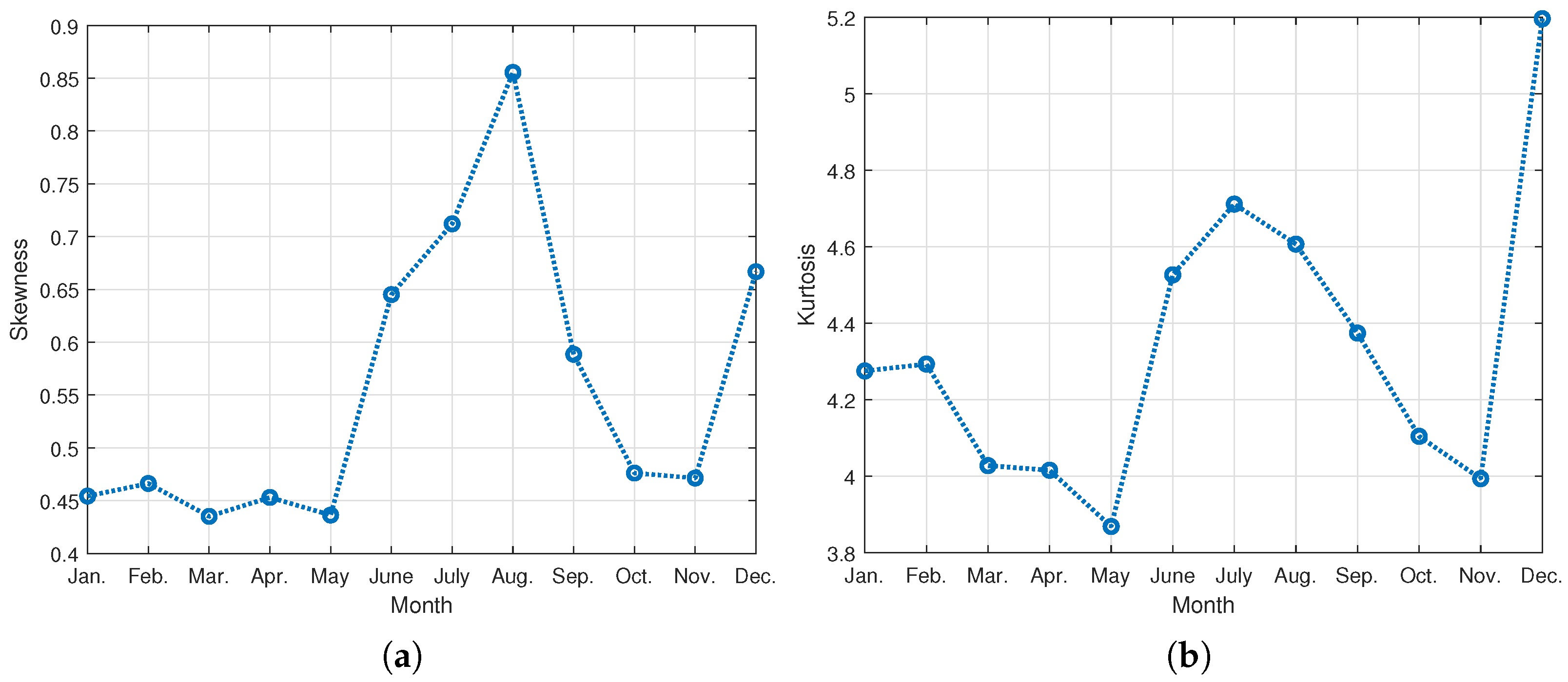
In order to conduct a quantitative investigation into the distribution of monthly electricity usage, we calculate the skewness and kurtosis values for each month. Skewness is a measure that indicates the degree of asymmetry of a distribution with respect to its mean [18,19]. A skewness value of zero suggests a symmetric distribution. On the other hand, kurtosis is a measure of the shape of the tail of a distribution in comparison to a Gaussian distribution. It provides insights into whether the distribution has heavier or lighter tails than a Gaussian distribution. In Figure 4, the results of skewness and kurtosis for twelve months are shown.
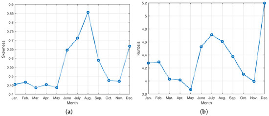
Figure 4.
Skewness and kurtosis of monthly electricity usage. (a) Skewness. (b) Kurtosis.
From Figure 4a, it is observed that the skewness values for each month are positive and less than 0.86. A positive skewness value means that it is right-skewed. When the skewness is between −1 and 1, it is considered that the distribution does not deviate significantly from symmetry [20]. From Figure 4b, the kurtosis values are found between 3.87 and 5.20. A Gaussian distribution has a kurtosis of 3 and a distribution that has fatter tails (more outliers) than a Gaussian distribution has high kurtosis. While it is suggested in [21] that a kurtosis value between −1 and 5 is considered to be close to Gaussian, there is no clear consensus for the range of kurtosis values that can be deemed to approximate a Gaussian distribution. However, a kurtosis greater than or equal to 10 is considered indicative of departure from a Gaussian distribution [22].
From the results of Figure 4, it is concluded that the distribution of monthly electricity usage does not exhibit notable asymmetry or heavy tails when compared to a Gaussian distribution. Let us denote a household electricity usage of month as . Based on our observations, we approximate the distribution of for nonnegative values by a Gaussian distribution as
where and represent the mean and standard deviation of monthly electricity usage, respectively. Table 3 shows these values calculated from the collected electricity usage data.
Table 3.
Mean and standard deviation of monthly electricity usage (kWh).
2.2. Analysis of Peak-Hour Usage Ratio of Households
The ratio of electricity usage during peak hours to total electricity usage varies depending on the lifestyle of household members, types of appliances used, and seasons. By analyzing usage data collected through AMI, the ratio of monthly peak hour electricity usage to total electricity usage is determined. Using the calculated ratio of peak-hour usage for each month, histograms are obtained for the twelve months. In Figure 5, histograms for the months of February, May, August, and November are shown as representative examples among the twelve months.
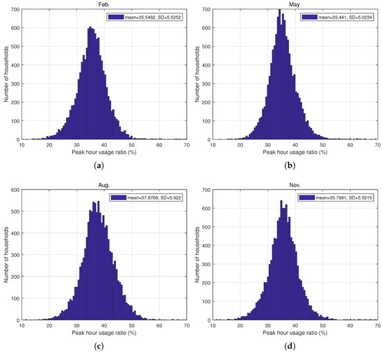
Figure 5.
Histogram of peak-hour usage ratio. (a) February. (b) May. (c) August. (d) November.
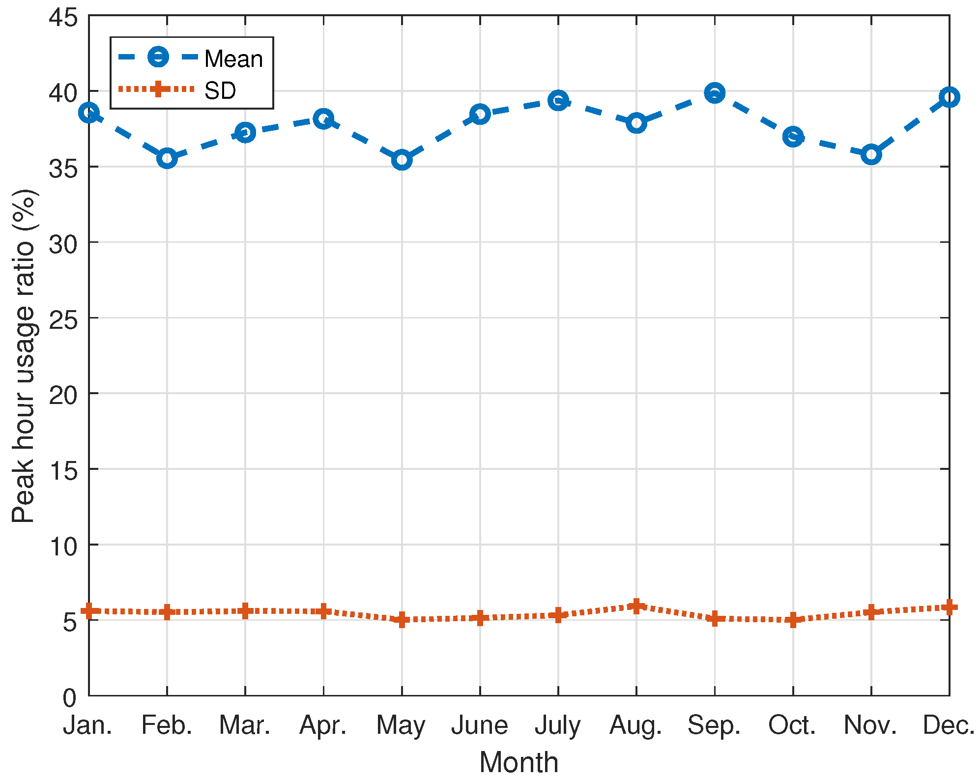
The horizontal axis in Figure 5 represents the percentage of peak hour electricity usage ratio, and the vertical axis represents the number of households with that usage ratio. The histogram shapes of the peak hour electricity usage ratio in February, May, August, and November are similar and exhibit a symmetrical pattern centered around the mean value. The mean values of the peak-hour usage ratio in February, May, August, and November are 35.5%, 35.4%, 37.9%, and 35.8%, respectively. The mean and standard deviation values for each month are shown in the top right corner of each graph. The histograms shown in Figure 5 are similar to the histograms of the peak-hour usage ratio for the other months. The mean and standard deviation values of the peak-hour usage ratio for the twelve months are shown in Figure 6. From the results, it is observed that there is not much difference in the mean and variance of the peak-hour usage ratio across different months.

Figure 6.
Mean and standard deviation of peak-hour usage values for each month.
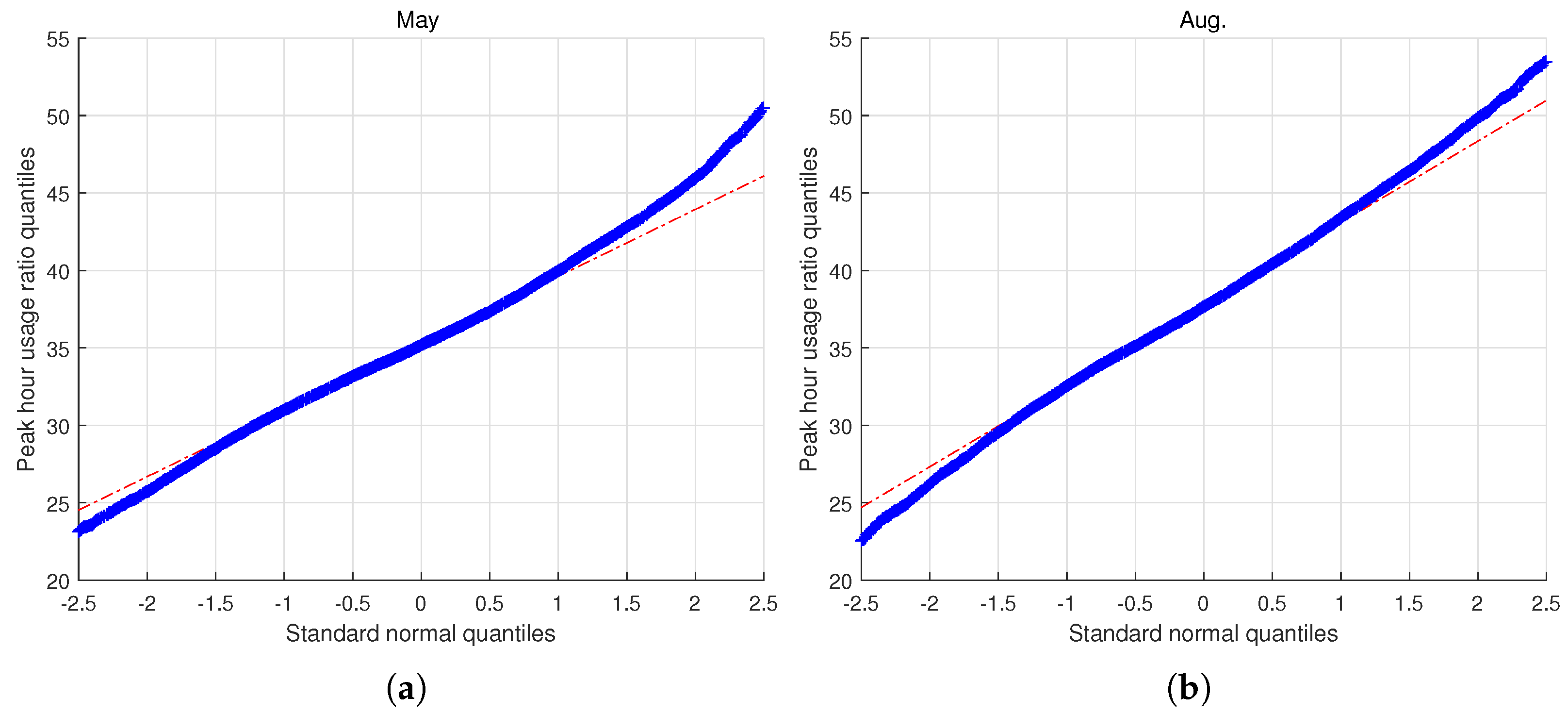
By observing Figure 5, it can be noted that the histogram of peak-hour usage ratio resembles a bell-shaped Gaussian distribution, with the mean value at its center, similar to the histogram of electricity usage. In order to further explore the resemblance between the distribution of peak-hour usage ratio and a Gaussian distribution, a normal Q-Q plot is obtained and shown in Figure 7. The normal Q-Q plots for all twelve months exhibit similar patterns, with May and August being used as representative examples in Figure 7.
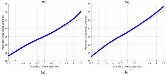
Figure 7.
Normal Q-Q plot of peak-hour usage ratio. (a) May. (b) August.
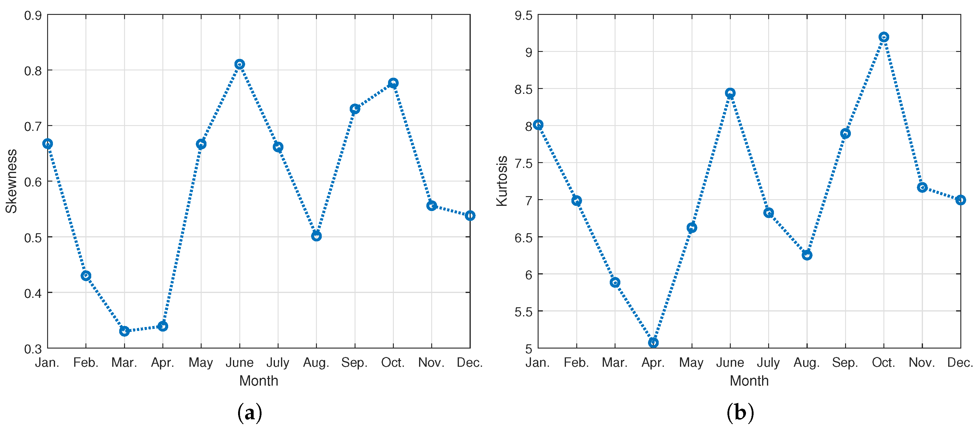
In Figure 7, blue markers fall below the red dotted line when the standard Gaussian quantiles are less than approximately −1.5 and rise above it when they are greater than approximately 1.0 in May or 1.2 in August. This indicates that the distribution has tails on both the left and right sides, with a relatively peaked shape. These characteristics imply that the distribution has a higher kurtosis value compared to a Gaussian distribution. In order to quantitatively examine the distribution of the peak-hour usage ratio, we calculate the skewness and kurtosis values for each month. The results of skewness and kurtosis for all twelve months are shown in Figure 8.
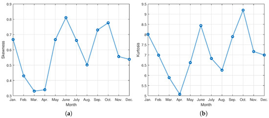
Figure 8.
Skewness and kurtosis of peak-hour usage ratio. (a) Skewness. (b) Kurtosis.
From Figure 8a, it is observed that the skewness values for the peak-hour ratio are slightly lower than those for the monthly electricity usage, and the kurtosis values for the peak-hour ratio are higher than those for the monthly electricity usage. However, it is still reasonable to conclude that the distribution for peak-hour usage ratio does not deviate greatly from a Gaussian distribution.
Let a household peak-hour usage ratio of month be denoted as . Then, the distribution of between 0 and 100 can be approximated by a Gaussian distribution as
where and represent the mean and standard deviation of peak-hour usage ratio, respectively. Table 4 shows these values calculated from the collected electricity usage data through AMI.
Table 4.
Mean and standard deviation of peak-hour usage ratio (%).
2.3. Correlation between Electricity Usage and peak-hour usage Ratio
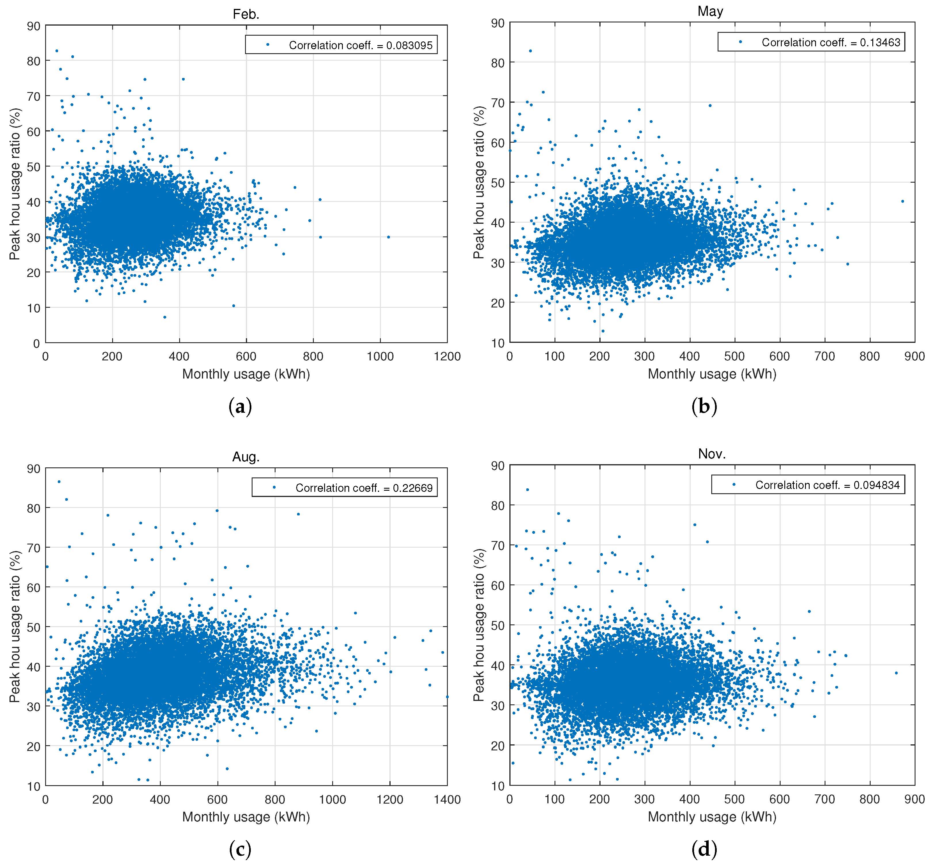
To analyze the relationship between the monthly electricity usage and the peak-hour usage ratio of households, all collected data of electricity usage and peak-hour usage ratio for each household are plotted in scatter diagram, shown in Figure 9. The scatter diagram results for February, May, August, and November are shown as representative examples. The horizontal axis represents the monthly electricity usage, while the vertical axis represents the peak-hour usage ratio. From the scatter diagram results of each month, it is observed that the points are widely scattered around a straight line, indicating a very low correlation between the two values. The calculated correlation coefficient value based on the actual electricity usage and the peak-hour usage ratio is shown in the upper right corner of the figure. The correlation coefficient values are found to be small, suggesting an almost uncorrelated relationship between the two values.

Figure 9.
Scatter diagram of electricity usage and peak-hour usage ratio. (a) February. (b) May. (c) August. (d) November.
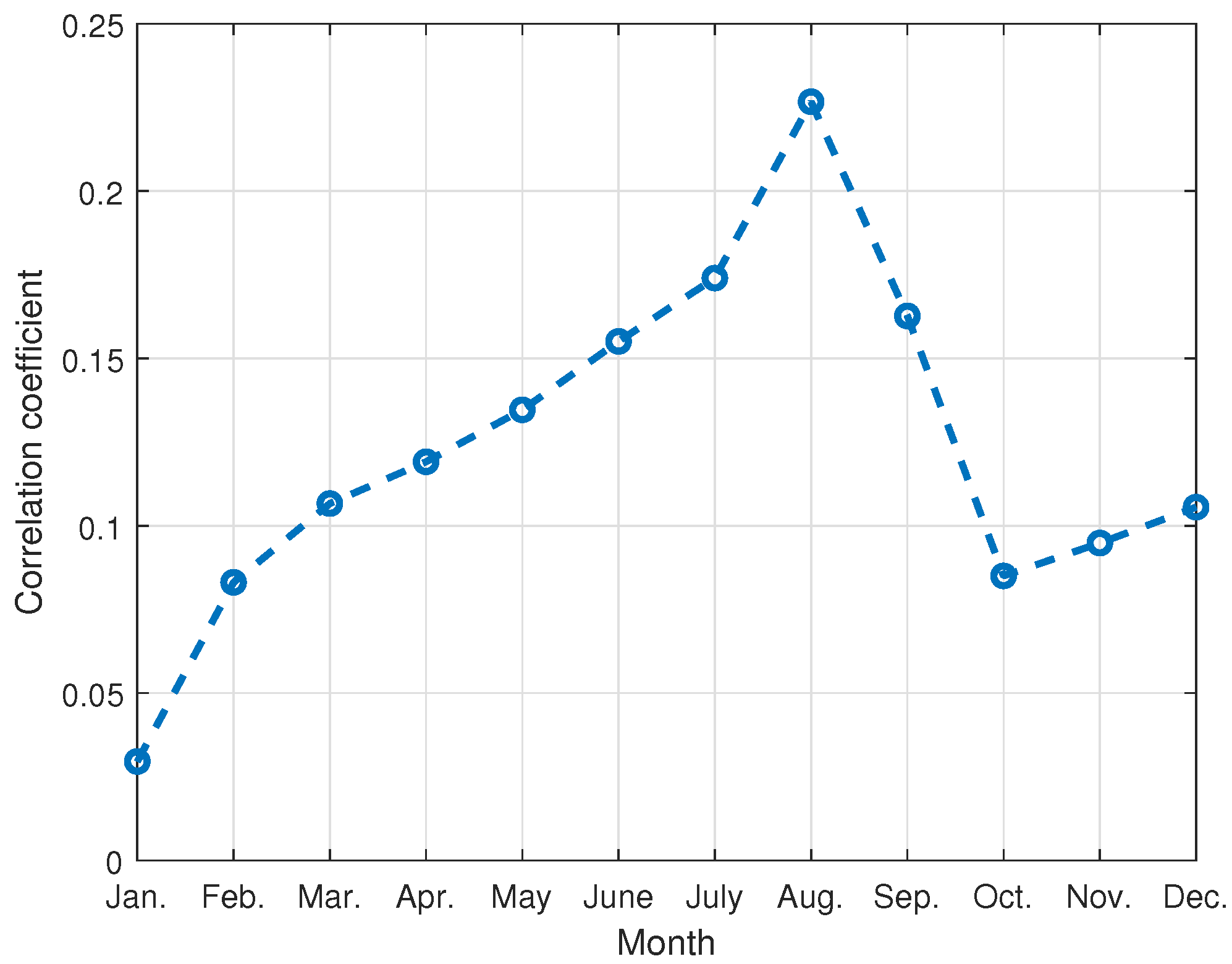
To further investigate the correlation, the correlation coefficient values obtained for every month throughout the year are shown in Figure 10. The correlation coefficient is highest in August, with a value of 0.23, while for the remaining months, the correlation coefficients are very small, below 0.17. Therefore, for the sake of simplicity in the following analysis, it is considered that there is no correlation between electricity usage and peak-hour ratio.
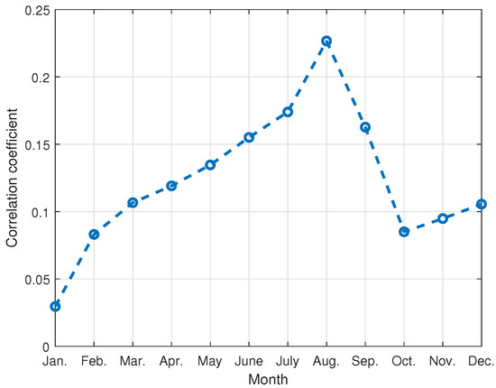
Figure 10.
Correlation coefficient values for each month.
2.4. Analysis for Average Monthly Bill by TOU Rate Plan
In this section, we analyze the statistical characteristics of household electricity bills from the perspective of average values when TOU rates are applied. First, we calculate the electricity bills by applying the TOU rate plans presented in Table 1. According to Table 1, the rates vary depending on the spring/autumn and the summer/winter cases. Let . For month k, the electricity consumed during peak hours is , resulting in a rate of . The electricity consumed during off-peak hours is , with a rate of . Therefore, for the spring/fall case, the electricity bill for month k is calculated as follows.
where and are defined in (1) and (2), respectively.
The monthly electricity usage and the peak-hour usage ratio are considered uncorrelated and are assumed to follow Gaussian distributions. Thus, the monthly electricity usage and the peak-hour usage ratio are independent random variables. This assumption leads to the calculation of the mean of the household electricity bills as follows.
where and are the mean of and , respectively. Similarly, we calculate the monthly household electricity bill for the summer/winter case. Let . For month k, the rate for electricity consumed during peak hours is , and the rate for electricity consumed during off-peak hours is . Thus, the electricity bill for month k is given by
and the mean of the household electricity bills is obtained as follows.
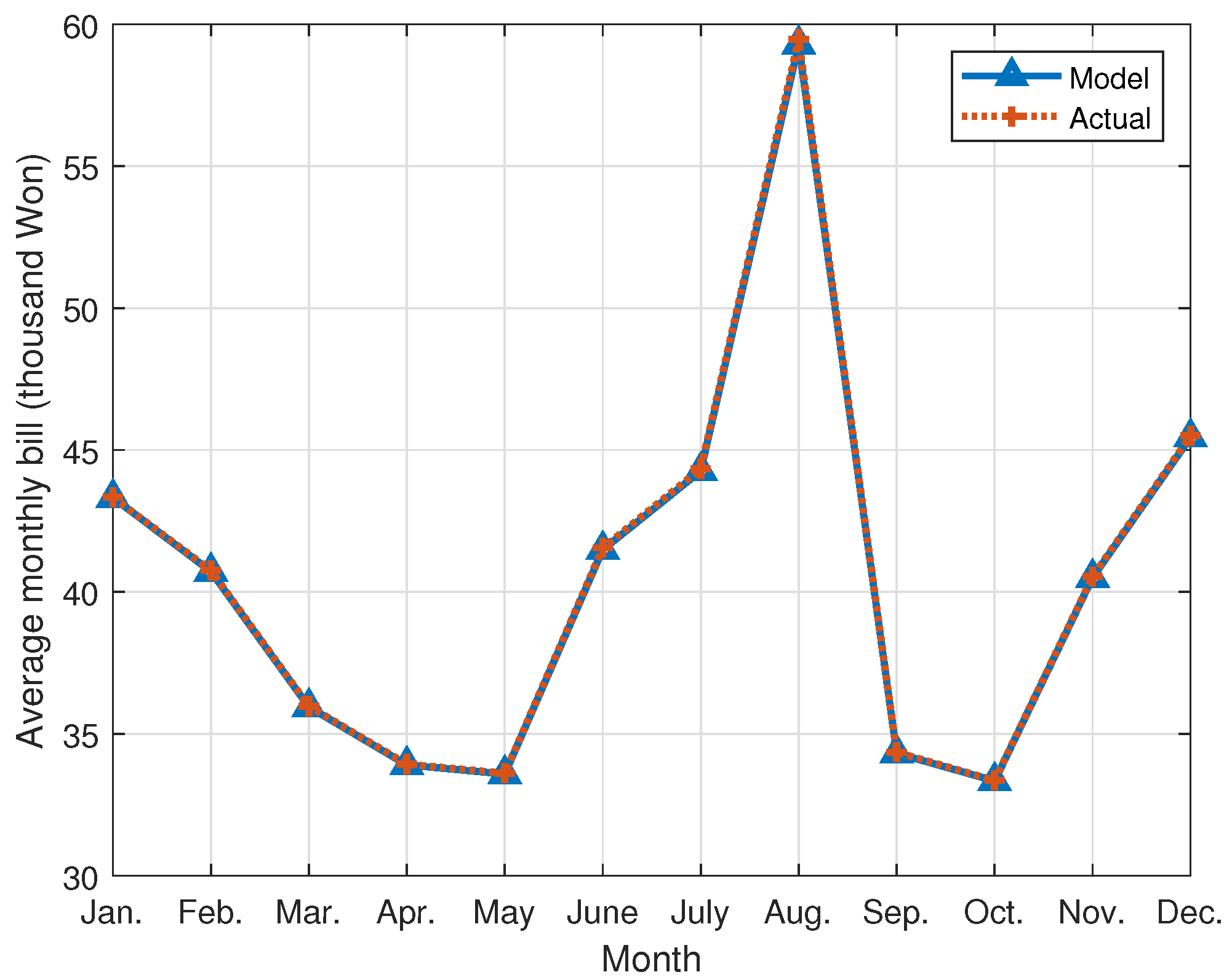
This statistical model is justified by comparing the actual average monthly bills of households obtained using all the collected data through AMI. In Figure 11, the average monthly bills for each household, calculated using the statistical model, are shown by blue solid line with triangle symbols. The actual average values of the household electricity bills, calculated using all the collected household electricity usage data through AMI, are shown by dotted line with plus symbols. Upon comparing the two sets of results, it is observed that there is almost no difference between the values obtained using the actual data and those obtained through the statistical model. The results show that an average absolute difference ratio with respect to the actual value is about 0.12%. Therefore, it is concluded that the statistical models for the average electricity bills of households, as given by (4) and (6), are valid.
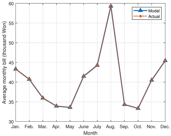
Figure 11.
Validation of the statistical model for the average monthly household bills.
2.5. Analysis of Bill Savings Obtained from Shifting Electricity Usage from Peak Hours to Off-Peak Hours
In a TOU rate plan, the electricity rates during peak hours are higher compared to off-peak hours. Therefore, even if the monthly electricity usage remains the same, shifting the electricity usage from peak hours to off-peak hours can result in a reduction in the electricity bill, leading to energy cost savings.
The ratio change by shifting the usage from peak hours to off-peak hours at kth month is denoted as percentage points (% points). As a result of this shift, the ratio of electricity usage during peak hours becomes %, while the ratio of electricity usage during off-peak hours is given by %. Using (3) and (5), the monthly household electricity bill with shifting electricity usage during peak hours is obtained as follows.
Therefore, the bill saving (in KRW) of a household for month k obtained by decreasing the peak-hour usage ratio by % points is as follows.
The annual bill saving for a household is obtained by
Then, the average of annual bill savings for households is as follows.
When the peak-hour usage ratio is decreased equally for every month, that is, for every k, , (10) is expressed as follows.
Using the values of in Table 3, is given by
Next, we analyze the average savings of the monthly electricity bills of households resulting from shifting kWh of peak-hour usage for month k. Again, the total electricity usage for the month remains unchanged. The decrease in the peak-hour usage ratio due to the shift to off-peak hours is as follows.
Note that from the result, depends only on . In other words, once is given, the value of is obtained deterministically. When the peak hour electricity usage is shifted to off-peak hours every month, that is, , for every k, (14) is simplified as follows. Again, the unit of is KRW.
3. Simulation Analysis on Shifting Home Appliance Usage Time
In this section, we select several home appliances for which usage time can be shifted and analyze changes in electricity bills when the usage time is shifted. First, let us consider the following representative home appliances:
- Electric washing machines (normal and drum washing machines);
- Clothes dryers.
In the case of an electric washing machine, the unit representing the amount of laundry is kilogram (kg) and the capacity of the washing machine is expressed as its standard washing capacity, which is the maximum load it can handle. It is recommended to load only half of the standard washing capacity to ensure effective drainage and optimal performance. A family of four in Korea typically washes about 3 kg of laundry per day. Assuming daily usage, the recommended washing machine capacity would be around 6 kg. Table 5 provides a summary of the energy consumption per wash of large-capacity (21 kg) and medium-capacity (14 kg) drum washing machines, both of which are highly preferred according to data from the Korea Consumer Agency (KCA, www.kca.go.kr, accessed on 1 October 2020) [23]. The laundry used for testing consists of 3.6 kg of cotton test cloth and 3.0 kg of blanket. We can observe that washing with the Futon course consumes the most energy, and the energy consumption increases when washing with hot water or at high temperatures. Note that the energy consumption for a single wash in Table 5 is subject to change depending on the washing conditions.
Table 5.
Electric washing machine energy consumption per wash [23].
In order to have more objective data on energy consumption, we use officially tested data based on the energy efficiency rating system implemented by the Korea Energy Agency (KEA, www.energy.or.kr, accessed on 27 April 2022), Republic of Korea. The Energy Consumption Efficiency Level Labeling System of the KEA is designed to facilitate consumers’ easy access to energy-saving products with high efficiency. Additionally, it enables manufacturers to make and market energy-saving products from the production phase. The labeling system is a mandatory reporting system based on laws, such as Articles 15 and 16, Energy Use Rationalization Act, Republic of Korea. In this system, the efficiency grades are classified into a scale of 1 to 5 according to energy consumption efficiency or energy consumption, with the minimum energy performance standard applied as the lower limit of energy consumption efficiency. Both domestic manufacturer and importers are obliged to display energy efficiency rating labels on their products, report their products, and comply with the minimum energy efficiency standard.
3.1. Usage Time Shift on Electric Washing Machines
In the case of an electric washing machine, the energy efficiency rating index , which means the amount of energy consumed per 1 kg of laundry, is defined as
In (16), (kg) indicates the capacity of the washing machine and is called the standard washing capacity. Consumers consider this standard washing capacity when purchasing a washing machine. In addition, (Wh) is the washing energy consumption when washing is performed once. The smaller the index value of , the better the consumption efficiency. Using this value, electric washing machines are rated in five grades. The rating standards for electric air conditioners, electric washing machines, and kimchi refrigerators were further raised on 27 April 2022 to display products with higher power efficiency.
When the monthly laundry frequency is times, the corresponding monthly energy consumption is
If (KRW/month) denotes the monthly electricity bill resulting from the usage, then can be written as
for an electricity rate of r (KRW/Wh). According to the Efficiency Control Equipment Operation Regulations, it is assumed that the monthly washing frequency is 17.5 times () in the case of electric washing machines. This corresponds 210 times a year. For example, with an energy consumption per 1 kg of Wh/kg, the annual electricity bill for the usage of this electric washing machine can be calculated. Given a standard washing capacity of kg and the electricity rate KRW/kWh in the peak hour of summer/winter in the TOU rate plan of Table 1, the annual electricity bill is KRW/year. To choose suitable electric washing machines for the simulations, we select the most recently certified products after 27 April 2022 based on the energy consumption efficiency rating system of KEA. We use their energy consumption per 1 kg for calculating the electricity bills. The selected electric washing machines are summarized in Table 6.
Table 6.
Electric washing machine energy consumption [24].
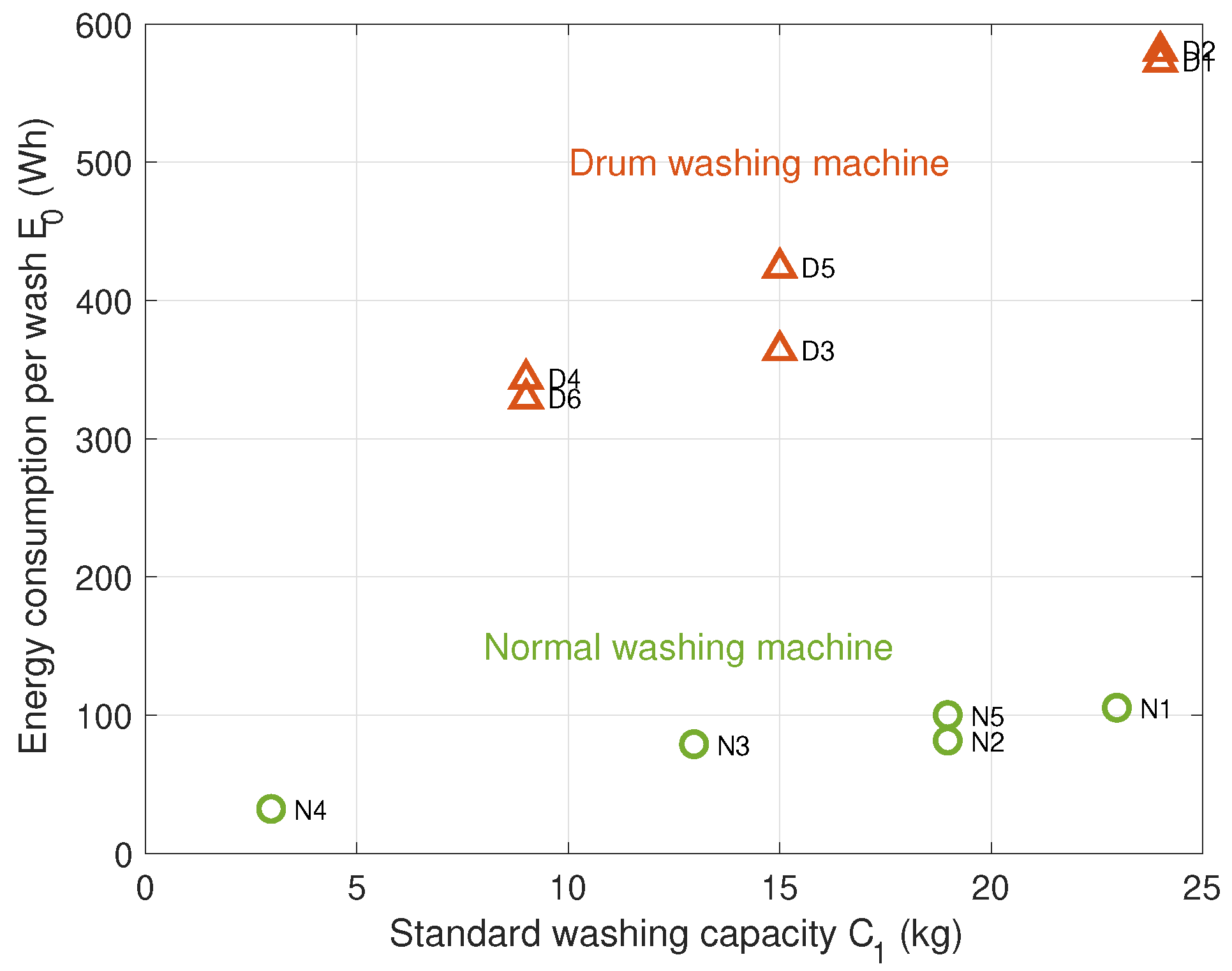
Figure 12 and Figure 13 show the energy consumption per wash and the energy consumption per 1 kg with respect to the standard washing capacities of the electric washing machines in Table 6, respectively. From Figure 12, we notice that the normal washing machines consume significantly less power than the drum washing machine case. Hence, we can also expect that the energy consumption per 1 kg of the normal washing machine is less than that of the drum washing machine. In Figure 13, the drum washing machines (D1–D6) exhibit higher energy consumption than the case of the normal washing machines (N1–N5), and the energy consumption per 1 kg decreases with an increase in the standard washing capacity. We can observe from Figure 13 that collecting some amount of laundry and washing it with an electric washing machine having a large standard washing capacity can reduce energy consumption.
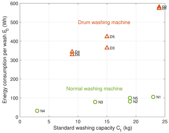
Figure 12.
Standard washing capacity of the electric washing machine and the energy consumption per wash in Table 6. The drum washing machines (D1–D6) consume more energy than the case of the normal washing machines (N1–N5).
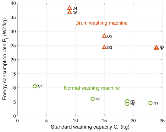
Figure 13.
Standard washing capacity of the electric washing machine and the energy consumption per 1 kg in Table 6. decreases as increases. In other words, collecting laundry and washing it with an electric washing machine with a large standard washing capacity can reduce energy consumption.
3.1.1. Shift of the Washing Machine Usage from the Perspective of Households
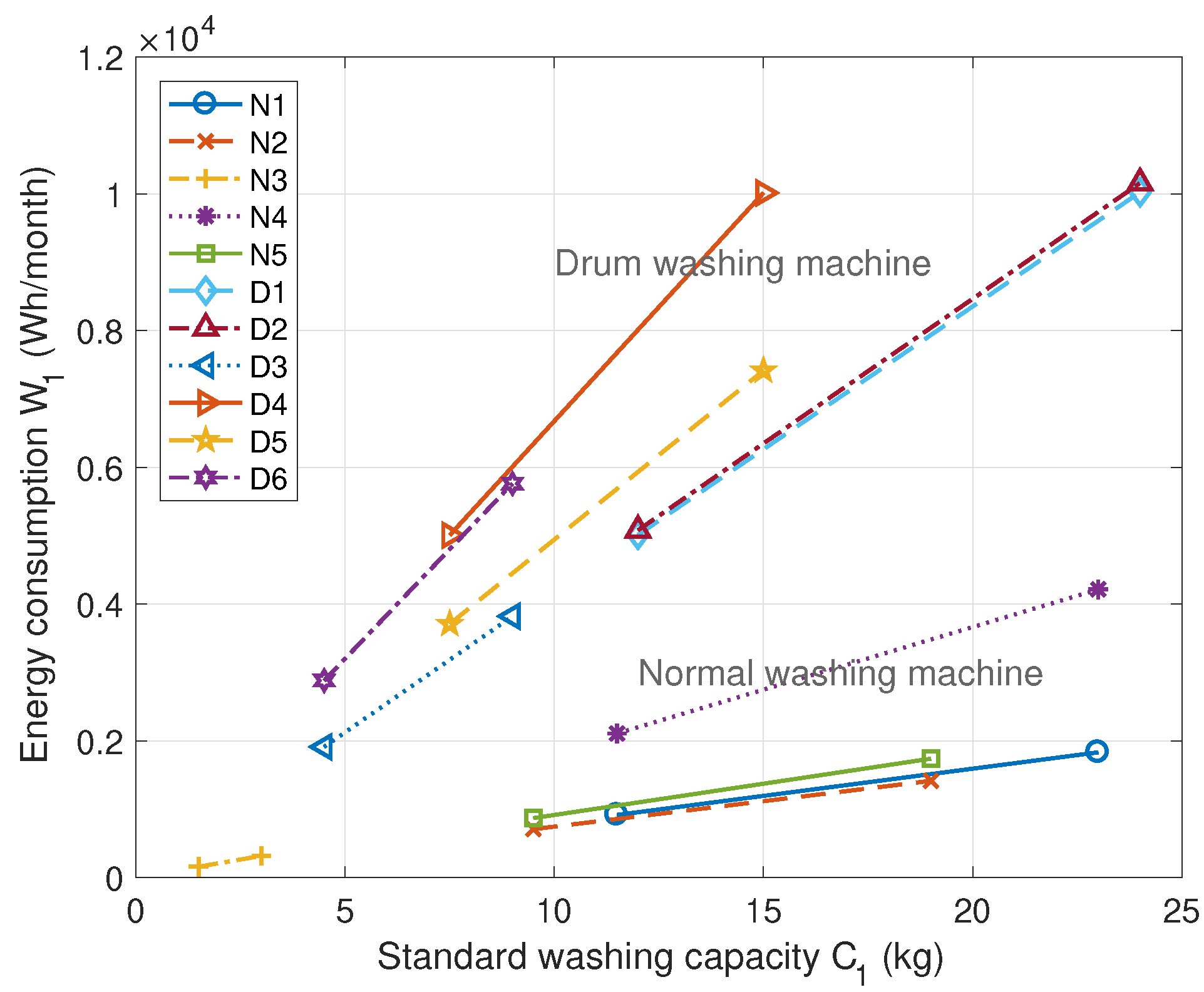
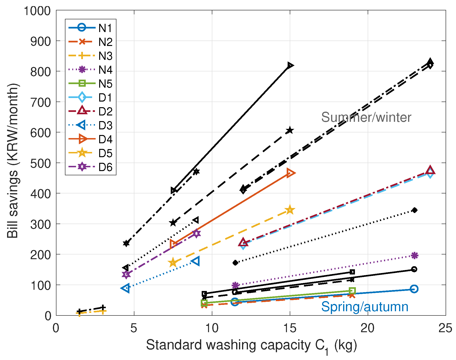
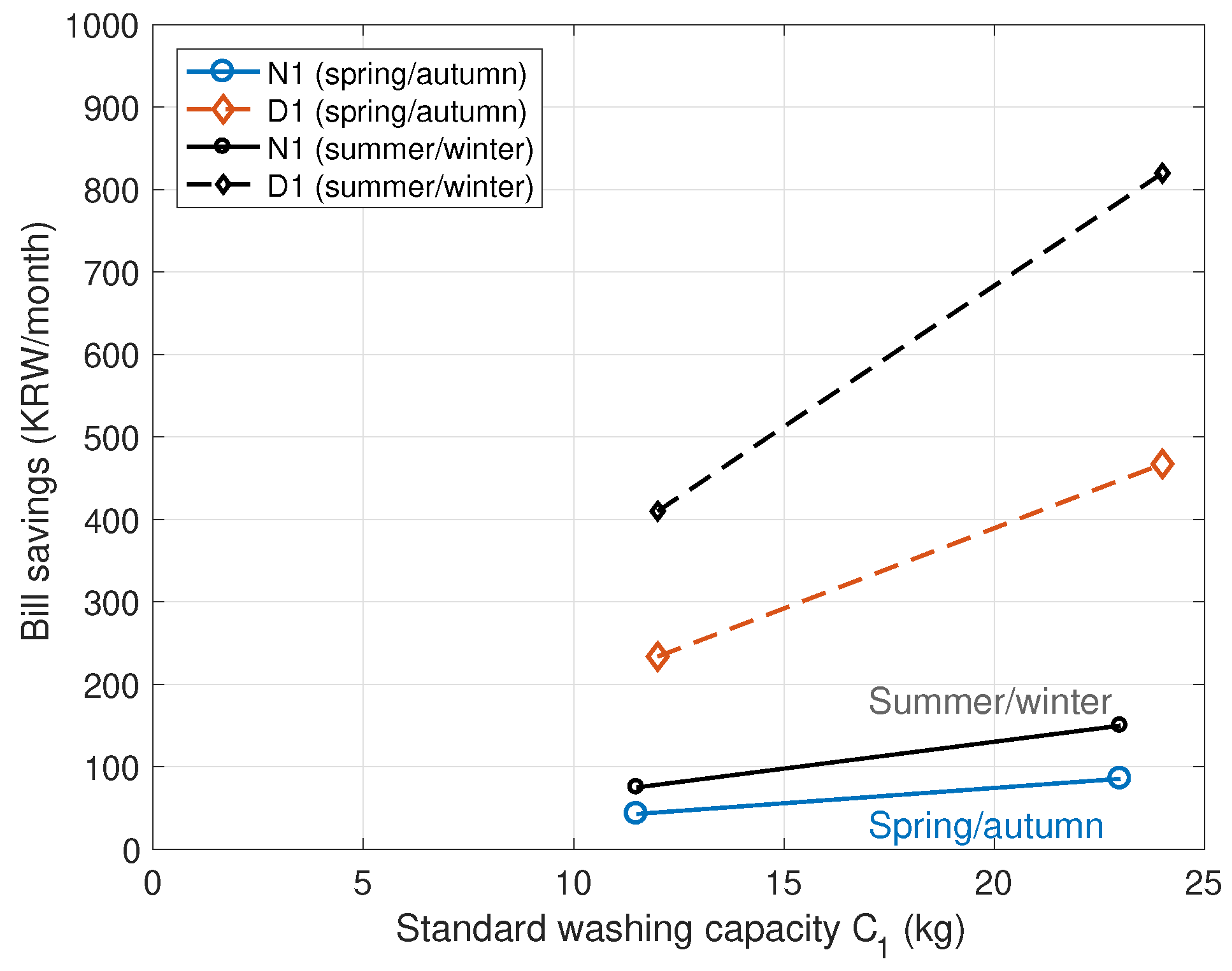
We first analyze the effect of the usage time shift from the perspective of households. In Figure 14, the monthly energy consumption of the electric washing machines in Table 6 is depicted for the standard washing capacity of (17). As the standard washing capacity increases, the energy consumption increases proportionally, and it can be seen that the annual energy consumption of the drum washing machine is larger than that of the normal washing machine. Figure 15 shows the bill savings achieved by shifting the usage time of the washing machine from peak hours to off-peak hours. The saved bill is obtained by calculating the electricity bill of (18) for both the peak and off-peak hours of the TOU rate plan, and then taking their difference. Figure 16 compares N1 (23 kg) and D1 (24 kg) as products with the highest energy consumption. For a standard washing capacity of kg of the drum washing machine D1, with and , the monthly energy consumption of (17) is kWh/month. From the TOU rate plan of Table 1 and (18), we can save KRW per month in spring/fall and KRW in summer/winter. On the other hand, for a standard washing capacity of 23 kg of the normal washing machine N1, KRW per month in spring/fall and KRW per month in summer/winter can be saved.
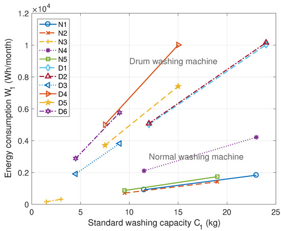

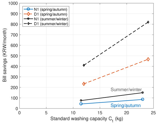
Figure 16.
Annual electricity bill saved by shifting the usage time of the washing machines N1 and D1 based on the TOU rate plan of Table 1. For a standard washing capacity of the electric washing machine D1 (24 kg), we can save about KRW 467 per month in spring/fall and KRW 820 per month in summer/winter.
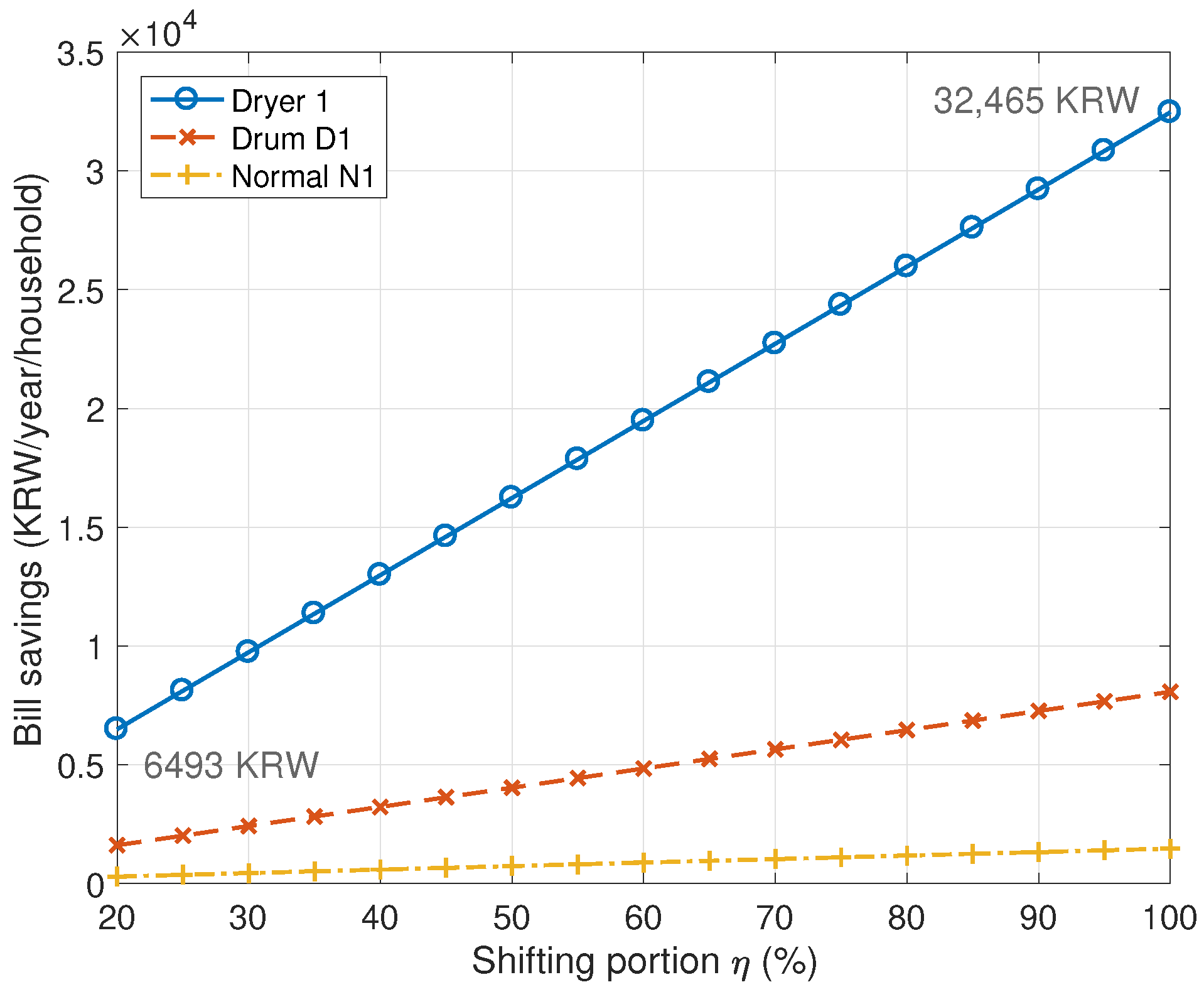
For the case of D1, if each household shifts the same energy consumption of kWh/month for 12 months, from (15), which takes into account all the seasons, the annual savings for each household is KRW. Figure 17 shows the annual savings of per household for the normal washing machine N1 and drum washing machine D1. The x-axis in Figure 17 means the annual shifting portion per household among 11,522 households in 10 apartment complexes, where holds and can be expressed as a percentage (%). It is clear that the bill savings increases in proportion to the shifting portion . Note that in Figure 17 a result for the clothe dryer is also shown for a comparison and will be introduced in the following section in detail.
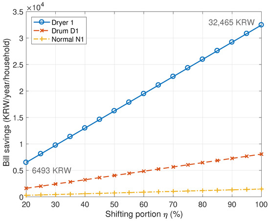
Figure 17.
Simulation of the electricity bill per household saved per year according to the shifting portion of the washing machines (N1, D1) and clothes dryer (Dryer 1) to off-peak hours. In the case of the clothes dryer Dryer 1, assuming that it is shifted %, we can save KRW 32,500 per household per year.
3.1.2. Shift of the Washing Machine Usage from the Perspective of Apartment Complexes
We now analyze the effect of the usage time shift to off-peak hours from the perspective of apartment complexes. The 10 apartment complexes in Table 2 have a total of 11,522 households, and the simulation was performed from (12) obtained by modeling the meter reading data from these households and the average and standard deviation of monthly electricity consumption in Table 3. From (12), the energy ratio change can be rewritten as
Hence, from (19), the bill savings for each household per year of the drum washing machine D1 yields points of the energy consumption shift to the off-peak hours. This calculation assumes that all 11,522 households in the 10 apartment complexes have made a complete shift. Note that this corresponds to the shift of kWh to the off-peak hours annually in 10 apartment complexes. If the shifting portion in an apartment complex is , then the actual energy ratio change can be written as
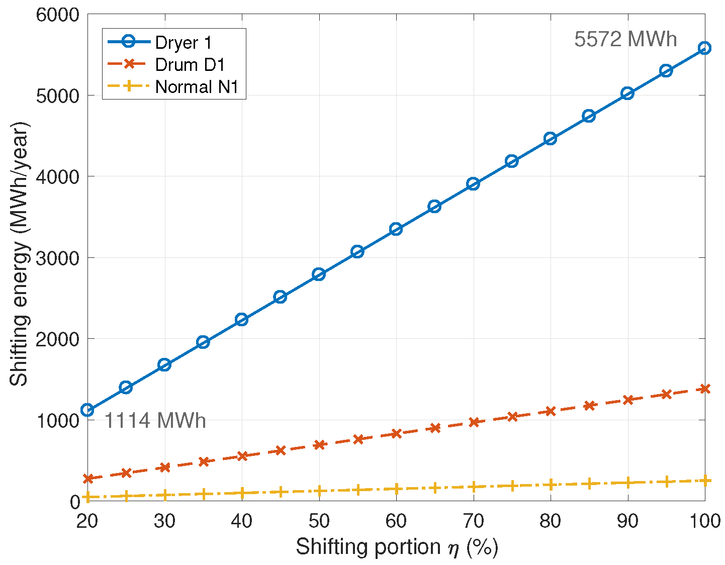
Figure 18 shows the ratio changes of for the normal washing machine N1 and the drum washing machine D1 with respect to the shifting portion . If the drum washing machine D1 shifts only % in 10 apartment complexes, then the shift corresponds to the energy consumption shift of kWh to off-peak hours annually. Figure 19 shows the shift of energy consumption (MWh) to off-peak hours with respect to the shifting portion of the normal washing machine N1 and the drum washing machine D1 in 10 apartment complexes.
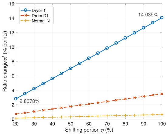
Figure 18.
Simulation of the energy ratio change to off-peak hours according to the shifting portion of the electric washing machines (N1, D1) and clothes dryer (Dryer 1). For the clothes dryer Dryer 1, assuming that it is shifted %, the energy ratio change becomes % points. This means that the average annual peak-hour usage in Figure 6 drops from 37% to about 23%.
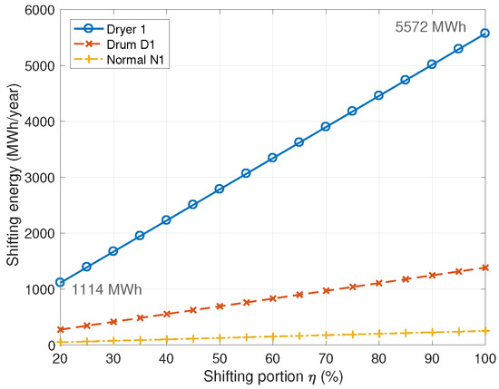
Figure 19.
Simulation on the usage time shifts of the electric washing machines (N1, D1) and clothes dryer (Dryer 1) to off-peak hours for the annual energy consumption of 10 apartment complexes.
3.2. Usage Time Shift on Clothes Dryers
In the energy efficiency rating label for the clothes dryer, the energy efficiency rating index (Wh/kg), which implies the energy consumption per 1 kg, is calculated by testing 3 times each with 2 sets of standard drying capacity and 2 half loads each with 2 test samples. This index is used to rate clothes dryers into five grades. Similar to the case of the washing machine in (17), the clothes dryer has the standard drying capacity (kg), which indicates the capacity of the clothes dryer. If the number of times of drying per month is , the monthly energy consumption is
If the monthly electricity bill is and the electricity rate is r (KRW/Wh), then can be written as
According to the Efficiency Control Equipment Operation Regulations, it is assumed that the clothes dryer is operated 13.3 times () in a month. This corresponds to 159.6 times a year. For example, with an energy consumption per 1 kg of Wh/kg, the annual electricity bill for the usage of this clothes dryer per year can be calculated. Given a standard drying capacity of kg and the electricity rate of KRW/kWh in the peak hour of summer/winter in the TOU rate plan of Table 1, the annual electricity bill is KRW/year. To select appropriate clothes dryers considered for the simulations, the most recently certified products are selected based on the energy consumption efficiency rating system of KEA, and their values of the energy consumption per 1 kg are used. The selected clothes dryers are summarized in Table 7. Figure 20 shows that the values of the clothes dryers in Table 7 improve as the standard drying capacity increases.
Table 7.
Energy consumption per 1 kg for clothes dryer [24].
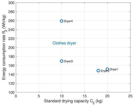
Figure 20.
Standard drying capacity and the energy consumption per 1 kg of the clothes dryers in Table 7.
3.2.1. Shift of the Clothes Dryer Usage from the Perspective of Households
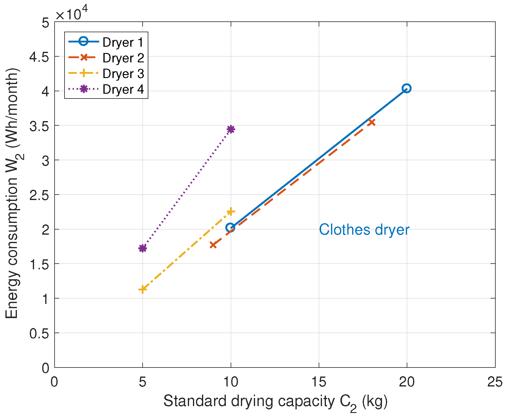
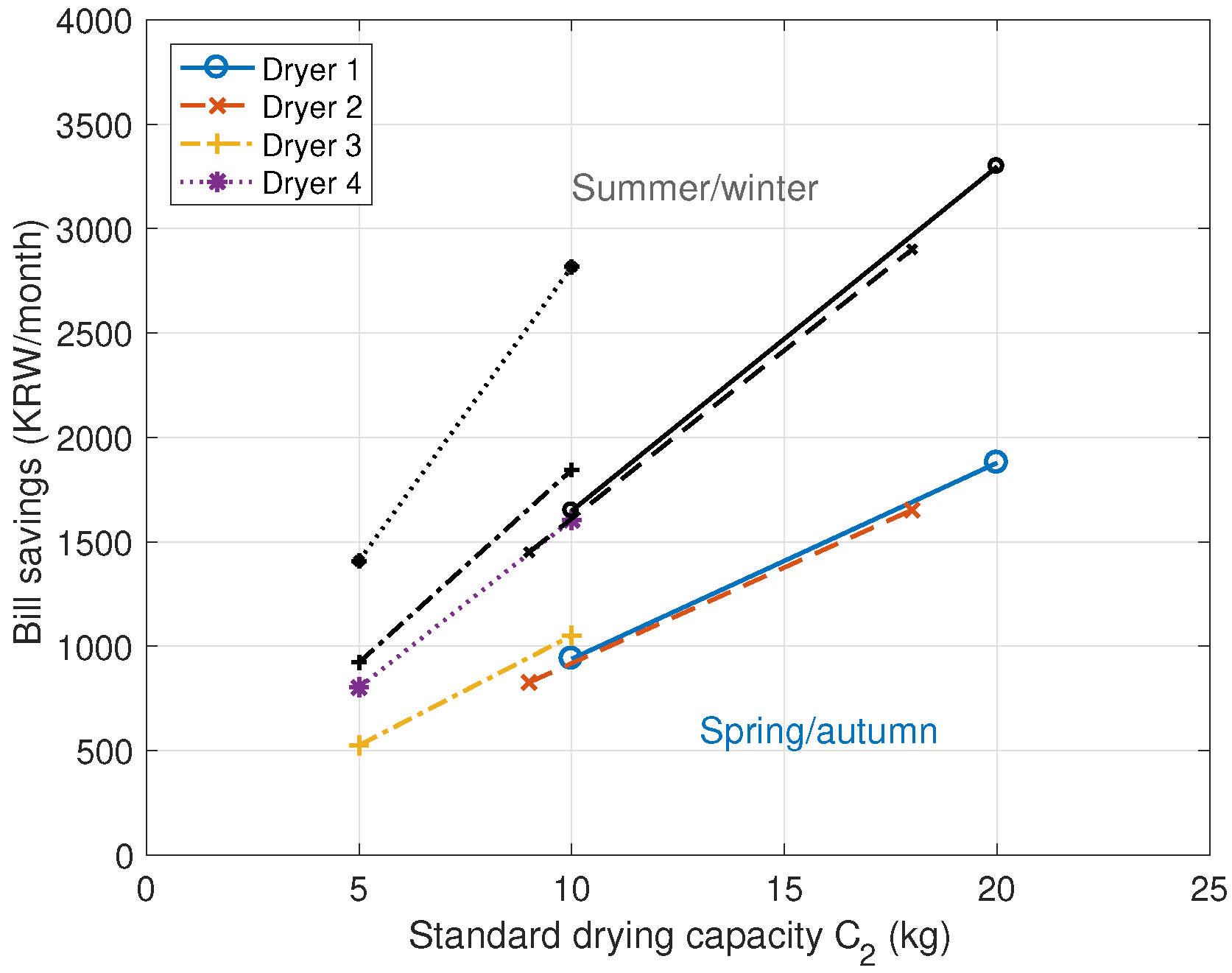
We first analyze the shift effect from the perspective of households. In Figure 21, the monthly energy consumption values of the clothes dryers in Table 7 are shown with respect to the standard drying capacity . Note that the energy consumption increases proportionally as the drying capacity increases. Figure 22 shows the bill savings when shifting the clothes dryer from peak hours to off-peak hours. The bill savings here are obtained by calculating the electricity bills in (22) for the peak and off-peak hours, respectively, and their differences.
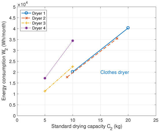
Figure 21.
Annual energy consumption with respect to the standard drying capacity of the clothes dryer in Table 7. In Dryer1 (20 kg), the monthly energy consumption is kWh.

Figure 22.
Monthly electricity bill savings when using a clothes dryer in the TOU rate plan are shifted to off-peak hours. Dryer 1 (20 kg) saves about KRW 1880 per month in spring/fall and KRW 3300 per month in summer/winter.
Let us look at Dryer 1 (20 kg) in Figure 20 with the largest standard drying capacity. Assume that the same energy consumption for 12 months in Dryer 1 is shifted 100% to off-peak hours. From Table 7, the standard drying capacity is kg and . Hence, from (21) and an assumption of , the monthly energy consumption is kWh/month. From the TOU rate plan and (22), we can then save KRW 3300 per month in spring/fall from . The bill saved from (15), considering all the seasonal factors, is about KRW per year. Figure 17 also shows the annual savings per household for Dryer 1. Compared to the electric washing machines N1 and D1, the energy consumption of the clothes dryer is greater, thus the bill savings are also large.
3.2.2. Shift of the Clothes Dryer Usage from the Perspective of Apartment Complexes
We now analyze the shift effect from the perspective of apartment complexes. Figure 18 also shows the ratio change of energy consumption in (20) for the clothes dryer with respect to the shifting portion . When %, KRW per household is saved for a year, and from (19), it means a statistical shift of about % electricity usage as shown in Figure 18. As observed from Figure 6, this shift implies that the ratio of energy consumption during average peak hours per year decreases from 37% to about 23%. As shown in Figure 19, assuming that all 11,522 households in the 10 apartment complexes adjust their usage time, a change of % results in kWh of annual energy consumption being shifted to off-peak hours in 10 apartment complexes. If only % of all households shift the usage time of the clothes dryer, about KRW per household can be saved annually. This is the case of subtracting 2.8% from the energy consumption during peak hours and shifting it by 2.8% to off-peak hours. In other words, as shown in Figure 19, it corresponds to a shift in energy consumption of about 1114 MWh per year in 10 apartment complexes. In addition, because clothes dryers consume more power than the electric washing machine case, shifting the usage time of cloths dryers has a greater effect on the efficient distribution of electricity usage.
4. Conclusions
In this paper, we first analyzed the statistical characteristics of customers’ electricity usage and their corresponding electricity bills under the TOU rate plan by investigating the electrical load profiles. We proposed a model for monthly electricity usage and peak-hour usage ratio of households based on the Gaussian distribution. We then derived an equation that yields an average of monthly electricity bills under the TOU rate plan. In Table 8, we next summarized several examples of the amount of electricity energy and electricity bill savings according to the usage time shift for each home appliance based on the derived equation. Compared to the electric washing machines, the energy consumption of the clothes dryer is usually greater, resulting in larger bill savings. For further practical analysis of electricity energy shift, it is necessary to investigate customer’s willingness to shift the usage time. If survey items are prepared by incorporating the contents of this paper regarding usage time, usage patterns, and shifts in peak hours for major home appliances, more reliable statistical data on shifts in electricity usage will be obtained. In addition, if detailed specifications of home appliances owned by each household and the usage patterns of these appliances are known during the survey stage, it would be possible to more accurately predict the amount of energy usage shifting to off-peak hours. This could lead to the development of an algorithm that calculates more precisely the amount of bill savings in each household. When analyzing the effect of shifting usage times, it is necessary to consider legal and noise-related issues that may arise due to the change in the usage times of home appliances. For example, there might be restrictions on running noisy washing machines or clothes dryers during nighttime in an apartment building environment. As various dynamic rate plans are expected to be presented in the future, comparing peak load shifting and electricity bill savings among these dynamic rate plans will help consumers select the rate plans that best suit their needs.
Table 8.
Simulation summary of bill savings and energy ratio change per household according to the usage time shift of home appliances to off-peak hours.
Author Contributions
Y.M.C. developed the model for monthly electricity usage and peak-hour usage ratio, conducted analyses and simulations, and refined the manuscript. B.J.C. derived the issues of analyzing bill savings with a TOU rate plan and organized and refined the manuscript. D.S.K. conducted analyses and simulations on shifting home appliance usage time and organized and refined the manuscript. All authors have read and agreed to the published version of the manuscript.
Funding
This work was supported by the Korea Institute of Energy Technology Evaluation and Planning (KETEP), the Ministry of Trade, Industry & Energy (MOTIE) of the Republic of Korea (No. 2021202090028D) and (No. RS202300236325). The work of Young Mo Chung was supported by Hansung University.
Data Availability Statement
Not applicable.
Conflicts of Interest
The authors declare no conflict of interest.
Abbreviations
The following abbreviations are used in this manuscript:
| AMI | Advanced metering infrastructure |
| DR | Demand response |
| KCA | Korea Consumer Agency |
| KEA | Korea Energy Agency |
| LP | Load profile |
| Q-Q | quantile-quantile |
| TOU | Time-of-use |
References
- Alberini, A.; Filippini, M. Response of residential electricity demand to price: The effect of measurement error. Energy Econ. 2011, 33, 889–895. [Google Scholar] [CrossRef]
- Torriti, J. A review of time use models of residential electricity demand. Renew. Sustain. Energy Rev. 2014, 37, 265–272. [Google Scholar] [CrossRef]
- Wu, Z.; Zhou, S.; Li, J.; Zhang, X.P. Real-Time Scheduling of Residential Appliances via Conditional Risk-at-Value. IEEE Trans. Smart Grid 2014, 5, 1282–1291. [Google Scholar] [CrossRef]
- Agnetis, A.; de Pascale, G.; Detti, P.; Vicino, A. Load Scheduling for Household Energy Consumption Optimization. IEEE Trans. Smart Grid 2013, 4, 2364–2373. [Google Scholar] [CrossRef]
- Kohlhepp, P.; Harb, H.; Wolisz, H.; Waczowicz, S.; Müller, D.; Hagenmeyer, V. Large-scale grid integration of residential thermal energy storages as demand-side flexibility resource: A review of international field studies. Renew. Sustain. Energy Rev. 2019, 101, 527–547. [Google Scholar] [CrossRef]
- Yahia, Z.; Pradhan, A. Multi-objective optimization of household appliance scheduling problem considering consumer preference and peak load reduction. Sustain. Cities Soc. 2020, 55, 102058. [Google Scholar] [CrossRef]
- Sadeghianpourhamami, N.; Demeester, T.; Benoit, D.; Strobbe, M.; Develder, C. Modeling and analysis of residential flexibility: Timing of white good usage. Appl. Energy 2016, 179, 790–805. [Google Scholar] [CrossRef]
- Mckenna, E.; Higginson, S.; Grunewald, P.; Darby, S. Simulating residential demand response: Improving socio-technical assumptions in activity-based models of energy demand. Energy Effic. 2018, 11, 1583–1597. [Google Scholar] [CrossRef]
- Mammoli, A.; Robinson, M.; Ayon, V.; Martínez-Ramón, M.; Chen, C.F.; Abreu, J.M. A behavior-centered framework for real-time control and load-shedding using aggregated residential energy resources in distribution microgrids. Energy Build. 2019, 198, 275–290. [Google Scholar] [CrossRef]
- Yilmaz, S.; Weber, S.; Patel, M. Who is sensitive to DSM? Understanding the determinants of the shape of electricity load curves and demand shifting: Socio-demographic characteristics, appliance use and attitudes. Energy Policy 2019, 133, 110909. [Google Scholar] [CrossRef]
- Verbong, G.P.; Beemsterboer, S.; Sengers, F. Smart grids or smart users? Involving users in developing a low carbon electricity economy. Energy Policy 2013, 52, 117–125. [Google Scholar] [CrossRef]
- Thimmapuram, P.R.; Kim, J. Consumers’ Price Elasticity of Demand Modeling With Economic Effects on Electricity Markets Using an Agent-Based Model. IEEE Trans. Smart Grid 2013, 4, 390–397. [Google Scholar] [CrossRef]
- Sergici, S.; Faruqui, A.; Powers, N. PC44 Time of Use Pilots: Year One Evaluation; Brattle Group: Baltimore, MD, USA, 2020. [Google Scholar]
- Yu, T.; Kim, D.S.; Son, S.Y. Optimization of scheduling for home appliance in conjunction with renewable and energy storage resources. Int. J. Smart Home 2013, 7, 261–272. [Google Scholar]
- Zhang, L.; Tang, Y.; Zhou, T.; Tang, C.; Liang, H.; Zhang, J. Research on flexible smart home appliance load participating in demand side response based on power direct control technology. Energy Rep. 2022, 8, 424–434. [Google Scholar] [CrossRef]
- Chung, Y.M.; Kang, S.; Jung, J.; Chung, B.J.; Kim, D.S. Residential electricity rate plans and their selections based on statistical learning. IEEE Access 2022, 10, 74012–74022. [Google Scholar] [CrossRef]
- Kim, D.S.; Jung, W.; Chung, B.J. Analysis of the Electricity Supply Contracts for Medium-Voltage Apartments in the Republic of Korea. Energies 2021, 14, 293. [Google Scholar] [CrossRef]
- Thode, J.C., Jr. Testing for Normality; Marcel-Dekker: New York, NY, USA, 2002. [Google Scholar]
- Doane, D.P.; Seward, L.E. Measuring skewness: A forgotten statistics? J. Stat. Educ. 2011, 19, 1–18. [Google Scholar] [CrossRef]
- Hair, J.F., Jr.; Black, W.C.; Babin, B.J.; Anderson, R.E. Multivariate Data Analysis, 7th ed.; Pearson Education Limited: Essex, UK, 2014. [Google Scholar]
- George, D.; Mallery, P. IBM SPSS Statistics 26 Step by Step: A Simple Guide and Reference, 16th ed.; Routledge: New York, NY, USA, 2020. [Google Scholar]
- Byrne, B.M. Structural Equation Modeling wih AMOS: Basic Concepts, Applications, and Programming, 2nd ed.; Routledge: New York, NY, USA, 2010. [Google Scholar]
- Electrical and Electronics Team. Drum Washing Machine Quality Comparison Test Result. Korea Consumer Agency. 2020. Available online: www.kca.go.kr (accessed on 1 October 2020).
- Electrical and Electronics Team. Efficiency Rating System. Korea Energy Agency. 2023. Available online: www.energy.or.kr (accessed on 27 April 2022).


Disclaimer/Publisher’s Note: The statements, opinions and data contained in all publications are solely those of the individual author(s) and contributor(s) and not of MDPI and/or the editor(s). MDPI and/or the editor(s) disclaim responsibility for any injury to people or property resulting from any ideas, methods, instructions or products referred to in the content. |
© 2023 by the authors. Licensee MDPI, Basel, Switzerland. This article is an open access article distributed under the terms and conditions of the Creative Commons Attribution (CC BY) license (https://creativecommons.org/licenses/by/4.0/).