Review

Identification of Free Components during Non-Simultaneous Complex Faults in Overhead Lines: A Review

Department of Power System and Control, Faculty of Electrical Engineering, Silesian University of Technology, 44-100 Gliwice, Poland
*
Author to whom correspondence should be addressed.
Energies 2023, 16(18), 6618; https://doi.org/10.3390/en16186618
Submission received: 31 July 2023 / Revised: 9 September 2023 / Accepted: 10 September 2023 / Published: 14 September 2023
(This article belongs to the Section F1: Electrical Power System)

Abstract

:
This study concerns the identification and interpretation of current and voltage signals during complex non-simultaneous disturbances in high-voltage overhead lines. It includes topics related to both the search for the optimal model of the system during complex disturbances as well as the analysis of the obtained results. The available EMT-like tools for the analysis of these phenomena are discussed. Models of high voltage overhead transmission lines are presented along with a discussion of their suitability for the study of electromagnetic transients during the analysis of complex non-simultaneous faults. Examples of transient waveforms of currents and voltages during non-simultaneous faults are presented, and the conditions for the occurrence of delayed current zero during short circuits in the system are discussed. The maximum values of the overvoltage factors and the conditions of their occurrence are described. Faults in transmission lines with various voltage levels suspended on the same supporting structures are discussed, together with an indication of the dangerous consequences of unusual intersystem faults. In the final part of the paper, the summary and recommendations for non-simultaneous fault studies are presented.

1. Introduction

Historical Review of Research

The inevitable consequence of faults in the power system, such as atmospheric discharges, phase-to-ground and phase-to-phase short-circuits, interruptions and switching operations, are transient waveforms, sometimes called balancing waveforms. The DC (aperiodic) components and the free components of higher frequencies are of considerable importance. The knowledge of free components occurring during electromagnetic transients is particularly important in two areas of research in power systems: ultra-speed protection systems and high-voltage apparatus and devices.
A special share of the DC component is contained in the current waveforms, in contrast to the free high-frequency components dominating in the voltage waveforms.
The amplitude, frequency and attenuation of free high-frequency components significantly affect the possibility of overvoltages in transmission systems.
These two types of components are significantly influenced by the non-simultaneity of faults.
The interest in non-simultaneous faults in high-voltage transmission systems was originally related to the issue of the increase in the current peak factor during three-phase non-simultaneous short-circuits. This problem arose during the study of delayed current zeros in currents during simultaneous three-phase short-circuits on the generator terminals [1,2,3,4,5,6].
The main reasons that may cause delayed current zeros during simultaneous short-circuits on the generator terminals are the operating conditions before the fault and the parameters of the generator. The influence of the power factor before the fault is important. As it was shown in [6], in the case of the capacitive power factor of generators, the time interval from the occurrence of the short circuit to the short-circuit first current is several times longer than in the case of an inductive factor. Delayed current zeros can also be caused by the underexcitation of the generators and the inequality of reactances in both axes of the machine. The inequality xd″ ≠ xq″ occurring in machines with salient poles without damping windings can cause the peak factor to reach significant values and, consequently, long delayed current zeros.
In the initial period of research, a significant impediment that allowed only a slight extension of the scope of the analysis was the lack of both appropriate models of the system and mathematical tools. Some computations were conducted with the use of analog machines [7,8], extending the research with the analysis of voltage signals in the highest voltage lines supplied on both sides. There was very little interest in non-simultaneous faults at that time, and even the few researchers limited the analysis to the study of peak currents [9,10,11], while the alarming results regarding the possibility of delayed current zeros—even for several periods—were considered as very unlikely.
Among scientists dealing with the problem of transients during faults in transmission lines, there are differences regarding the modeling of the system and the interpretation of signals, resulting from both the method of solving and the type of approach (deterministic or probabilistic) to this problem. The existence of these discrepancies is an obvious result of the difficulties encountered in the study of transient phenomena in identifying and modifying equivalent circuits resulting from the reduction in primary systems. Of course, the question may arise of why reducing the system at all, since we have a certain number of applicable programs at our disposal, which can be used to perform calculations in systems containing several thousand nodes. Conducting calculations in an extended original system will always lead to doubts regarding the desirability of the accurate modeling of each of the elements, or the scope of system simplifications and their impact on the reliability of the obtained results [12]. The identification of equivalent circuit parameters is possible using the Netomac program [13].
The proponents of the probabilistic approach have attempted to convince other researchers that multiphase faults should be treated as simultaneous ones.
Treating multiphase faults in high-voltage transmission lines as simultaneous is, with the exception of a two-phase fault, incorrect not only for the analysis of the transients of currents and voltages. The standards constituting the basis for determining the requirements for electrical devices, as well as in the selection of power protection automatics, ignore the effect of non-simultaneity on the maximum values of currents and voltages that may occur during these faults. When analyzing the causes of multiphase short circuits in HV lines, there are two main reasons for the occurrence of this type of fault: an electric arc and closing of a faulted line by the circuit breaker during a failed auto-reclosing cycle. An electric arc is unlikely to cause a fault to start simultaneously in several phases. A special, very rare case should also include the simultaneous closing of all poles of the circuit breaker.
In the case of treating the mechanical non-simultaneous closing of individual circuit breaker poles as the cause of non-simultaneous faults, the modeling of the faults is a simple matter. For these cases, calculations were condcuted (especially in countries with difficult access to computing centers) on an analog machines, which at that time competed with large digital machines primarily in terms of calculation speed.
In the case of the studies of voltage transients during non-simultaneous faults, the situation was more complex due to the need to find a reliable model of a high-voltage transmission line.
Computational analysis, even with the use of digital technology, is currently possible thanks to access to numerous applicable programs.
An overview and evaluation of the available programs for calculating transient states in transmission lines can be found in [14]. Most good programs are EMTP-like, which are designed for a high-precision study of the power system through the reproduction of actual time-domain state variable waveforms at any selected location in the system.
The history of the creation and development of the EMTP program is very well described in [15]. The basic theory and development of EMTP was explained and the existing EMT-type tools were described, among which the currently available and most often used in the study of transients in transmission lines can be distinguished as follows:
  • ATP-EMTP [16], popular especially among individual scientists.
  • EMTP® [17], a very advanced simulation tool with load-flow initialization; here, a very accurate frequency-dependent wide-band line (or cable) model is available.
  • MicroTran [18], mainly (but not only) for students of the University of British Columbia, very user-friendly. Applied in over 25 countries.
Taking into account all the mentioned factors, it can be argued that, for each power transmission system, it is possible to perform electromagnetic calculations of transients during complex non-simultaneous faults. A pre-requisite for proving this thesis is the proper reflection of the parameters of this system—especially the transmission line.
The line model should have an extended form, necessary from the point of view of calculation accuracy, with acceptable simplifications, possible due to the negligible impact of other parameters.
The study covers three groups of issues related to the identification of transmission systems during complex disturbances in the system. The first of them (Section 2) concerns the selection of calculation tools and models of transmission systems (HV lines) from the point of view of the best reconstruction of free current and voltage components.
The second group of issues is (Section 3) the conditions and meaning of free components in current and voltage waveforms.
The last thematic group is directly related to the interpretation of the analysis results obtained in test systems.
The content of Section 4 and Section 5 results from the order of the work objectives. Tests for current (Section 4) and voltage (Section 5) waveforms were conducted separately. The testing of DC free components for currents and hf for voltages was omitted due to the negligible effect of hf for currents and DC for voltages.
The Section 6 presents the results of the analysis concerning the impact of the non-simultaneity of disturbances on instantaneous waveforms and the maximum values of currents and voltages in lines with various voltage levels operating on the same supporting structures. This is a new issue—there are no publications on the subject, and the research results to date are very dangerous (intersystem faults). This problem will increase due to the inevitable—forced by economic and organizational reasons—increase (expansion) in this type of transmission lines.

2. Optimal Model of High-Voltage Transmission Lines in Fault States

2.1. Principles and Conditions

The requirements for the transmission line model resulted from the need for the accurate reflection of transients during complex faults containing free higher-frequency components.
In fact, the line is the only element of the power system with evenly distributed parameters. Therefore, computer studies of transient states in lines require the use of appropriate numerical methods.
Currently, the following transmission line models are available in EMT-like programs:
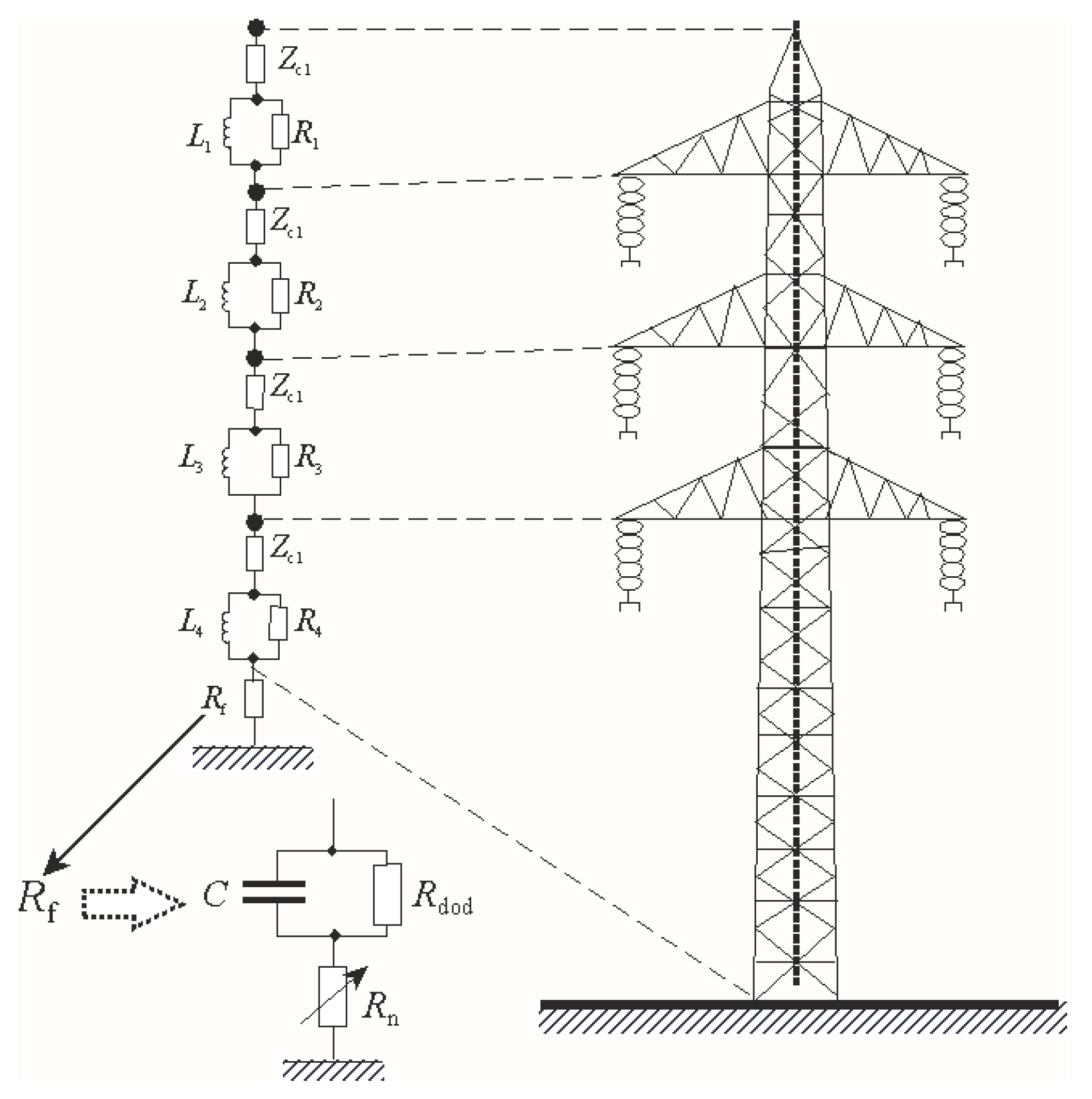
  • Lumped-parameter (π-equivalent) circuit model [18], which is accurate only at the frequency at which the parameters are evaluated. One π-circuit can serve as a representation of only one natural resonant frequency of the considered circuit (in most cases: the power system frequency, i.e., 50 or 60 Hz). When consisting of k-sections of π-circuits, k natural frequencies can be represented, although the amplitude is accurate only for the first one. The whole line is divided into n sections, where the parameters of each have a ratio of 1/n in reference to the line constants of the whole line. For steady-state calculations, this representation is reasonably accurate if each π-circuit is not too long. The equivalent transmission line model of the cascaded π-shape required corrections for long transmission lines (approximately 200 to 250 km in length).
  • Lossless distributed line model [18] can represent traveling-wave behavior but is valid only for the frequency at which the parameters are computed. Several natural resonant frequencies are represented approximately for an open-circuited line. The accuracy of this model decreases when considering matching and short-circuited lines in a high-frequency region.
  • JMarti model [19] (FD)—in the modal domain—is used in many applications in EMT-like programs (however, in this paper, the frequency-dependent transformation matrix was neglected). Despite this imperfection and any critical remarks, there is a sufficiently good match between the FD model and other models (and a good agreement with measurements).
  • Frequency-dependent line model in the phase domain. To avoid the numerical instability by the use of FD [20], a phase-domain line model was established [21,22]. This approach has become the most accurate frequency-dependent wide-band line model in EMTP®. A drawback is that software coding and advanced numerical computations are required.

2.2. Line Modeling including the Influence of Higher Frequencies

Almost all modern computer programs that are applied to calculate the parameters of high-voltage lines use Carson’s rule [23]. A number of methods derived by different authors are an extension of this rule, with the obtained results differing from each other by a maximum of 10% (in the 100 Hz to 10 kHz range). For the analysis of transients containing components with higher frequencies (>100 kHz), the influence of soil heterogeneity should be additionally taken into account. On the basis of research into the problem of the inhomogeneity of deeper layers of the Earth, the negligible impact of this phenomenon on the results of the calculations of electromagnetic transients during short-circuit faults was demonstrated [24].
The calculations show that the values of unit resistances—especially for the zero component—increase very strongly with a rise in the frequency; the unit inductance of the line depends to a very small extent on the frequency, and the obvious fact is that the unit capacitance of the line does not change with the increase in the frequency.
Depending on whether the line is modeled with the use of lumped or distributed parameters, additional circuits are used to take into account the influence of higher frequencies on the line parameters. In the case of line modeling using a chain of substitute elements, the most advantageous solution from the point of view of the minimum number of additional equations is the system shown in Figure 1 [25]. On the basis of the given characteristics of the dependence of the line parameters on the frequency and by using the Newton–Raphson numerical method, the above-shown equivalent circuit of series-connected parallel RL circuits was obtained, the number of which depends on the required approximation range.
A number of papers used such solutions; e.g., in [26], the frequency dependence was introduced in the mode domain through the use of modified π-circuits, where the frequency dependence of the longitudinal parameters was reflected through the use of RL series circuits with the addition of RL parallel circuits. The impedance for this circuit is expressed through Equations (1) and (2), where R1,k, L1,k, … are the sought substitute parameters for the approximation of the nonlinear relationship.
R ω = k = 1 n R 1 , k R 2 , k R 1 , k + R 2 , k + ω i 2 L 1 , k 2 R 2 , k + L 2 , k 2 R 1 , k R 1 , k + R 2 , k 2 + ω i 2 L 1 , k + L 2 , k 2 ,
ω L ω = k = 1 n ω i 2 L 2 , k R 1 , k 2 + L 1 , k R 2 , k 2 + ω i 2 L 1 , k L 1 , k + L 2 , k R 1 , k + R 2 , k 2 + ω i 2 L 1 , k + L 2 , k 2 ,
When modeling the line with the use of lumped parameters, one can recall that the frequency of the free component, which is to be reasonably accurately reflected, must be lower than the natural frequency of a single π-circuit. It is known that an increase in the number of π-circuits causes an increase in the correspondence between the natural frequency of the line modeled with the distributed parameters and the chain of π-circuits. However, the lowest-frequency components that are dominant in the transients can be represented, with sufficient accuracy, by means of a system consisting of several π-circuits. On the other hand, when the number of π-circuits in the system is doubled, the highest natural frequency of the system also increases approximately twice. Since the highest frequency of the computed waveform determines the required computation step (with an increase in the number of π-circuits, there is an increase in the number of equations in the system—in consequence, the computation time is longer), when using the method of numerical integration of the implicit function, it should be assumed that the line is modeled using the smallest possible number of π-circuits. Especially when the line parameters should depend on the frequency, it is possible that, when increasing the number of π-circuits, components appear in the line model that are not present in the real system at all. One can also recall that the appearance of new (fictitious) components is caused by capacitances at the beginning or at the end of the circuit, together with the established inductances.
The comparison of the voltage transients computed for the same operating conditions in the system and different line models best illustrates the considerations mentioned above. The transient waveform of the L1 phase voltage at the beginning of the line presented in Figure 2 was obtained during the short circuit of this phase to the Earth at the end of the line. The waveforms shown were obtained for the same short-circuit conditions for the line modeled with one and one hundred three-phase π-circuits, taking into account all capacitive and inductive couplings.
As it can be seen, increasing the number of substitute elements causes an increase in the amplitude of the higher frequency components. In addition, the damping time of these components increases. Taking into account the additional factor of extending the computation time caused by the increase in the number of differential equations describing the system, this manner in which the transmission line could be modeled during the numerical analysis of transient states should be absolutely rejected. In cases where it is necessary to model the line using lumped parameters, the number of π-circuits should be limited to a minimum, while the number of equations “saved” in this way can be “used” for damping systems.
For the line model with distributed parameters, the frequency dependence of the parameters is taken into account by using, for example, the Marti model, where the approximation of the dependence of the impedance on the frequency is applied using a system of chained RC elements.
Marti’s model has been modified in subsequent versions of EMTP programs, and in contrast to the trapezoidal numerical method applied in the source program, the numerical integration of an implicit function is used, while the method is based on recursive convolution, although there is no agreement among the authors of the EMTP program regarding whether this method is better than the trapezoidal method [18].
Figure 3 depicts a comparison of the voltage transients and the beginning of a 10 km and 200 km line, during a non-simulatenous three-phase fault at the end of the line modeled using the Marti model and a cascade connection using one and one hundred π-circuits.
The qualitative and quantitative errors of the results (of the voltage waveforms at the beginning of the line during a short circuit at its end) obtained using the line model with distributed parameters independent of the frequency are shown in the comparison in Figure 4. In the voltage waveform obtained in a system with a line represented by frequency-dependent parameters, after 80 ms, there are practically no free components of higher frequency, while the voltage waveform at the same time obtained in a system with a line represented by constant parameters is very distorted due to the presence of components with a significant amplitude. The differences in the voltage amplitudes are significant: for the model with constant parameters, the maximum “peak” of the instantaneous voltage is 1.3 in contrast to the model with parameters dependent on the frequency, where no overvoltages occur.
The omission of the dependence of the line model parameters on the frequency is an error that results in incorrect quantitative results—this applies to the amplitude and damping time of the free high-frequency components—as well as qualitative. As a result of the overlapping of components with different contributions, a waveform significantly different from the real one is obtained.
The modeling of a line with the use of a cascade connection of π-circuits with lumped parameters during the analysis of electromagnetic transients can only cause additional problems, the elimination of which (through additional compensating systems) may unexpectedly become one of the main tasks of this analysis. Regardless of the dubious results of achieving “optimal” line modeling with such a system, the computation time is significantly extended.
The line model based on a cascade connection of π-circuits is excluded for the analysis of phenomena during non-simultaneous faults, which does not mean a disqualification of this solution and successes in the study of other phenomena [26,27,28].
It can also be an obvious mistake not to include the skin effect in the line model, especially for phase-to-phase faults without the ground.
The model of the overhead line for the study of “microsecond” phenomena must take into account the phenomenon of dynamic corona by introducing additional equivalent systems [29]. In addition, the model of the supporting structure as a multistory transmission tower model to be used in the multi-conductor analysis in EMTP [30] must be taken into account. A schematic diagram of such a structure is shown in Figure 5. The circuit parameters of the model are determined basing on voltage measurements across the insulator strings on an actual 500 kV transmission tower.
The use of such a model in the millisecond range is unnecessary. As it was shown in some of the results cited above, the decisive factor in considering the dynamic corona effect in the line model is the multiplicity of the initial corona voltage during the tested transients. For example, for the analysis of atmospheric or switching overvoltages, such a system should be introduced. Supplementing the line model in other cases extends the computation time and enlarges the set of input data.
The accurate modeling of the nonlinear character of the short-circuit arc (as a dynamic arc with hysteresis loops) is necessary in particular studies of transient phenomena occurring during a voltage-free interruption in the single-phase or three-phase auto-reclosure cycle.
For non-simultaneous, slow-developing arc faults, e.g., when phase conductors touch the top of a tree, arc modeling can be used according to a nonlinear static characteristic (time-varying resistance) [31,32,33].

3. Importance of Free Components during Faults

The inevitable consequence of faults in the power system, such as atmospheric discharges, phase-to-ground and phase-to-phase short circuits, breaks and switching operations, are transient waveforms, sometimes called balancing waveforms. In fact, a theoretical analysis is almost never conducted for the entire duration of the fault. To be more precise, depending on the need for information about specific quantities in the system during a fault, the analysis is limited to the appropriate time range in which it is to be conducted. For these contractual time ranges, appropriate models of power system elements apply. Therefore, which of the models are to be used in the appropriate analysis is determined by the frequencies of the components occurring in the transients, as shown in Figure 6.
The division of transients shown in Figure 6 is conventional both in terms of limit frequencies, which are smooth, and in terms of assigning appropriate models of system elements to specific states. It is difficult to imagine a justification for a sudden change in the model of a given element at a specific time point counting from the beginning of the fault occurrence. When reviewing the literature, it is also possible to notice different cut-off frequencies for transients and the corresponding models [1,13]. Of course, from the point of view of the capabilities of currently available computers, the use of single, most complex models, possible of using during the entire duration of the fault, is not the slightest problem. However, taking into account the properties of the power system, more precisely, the behavior of individual elements during the transient state, a universal model of the system for the entire frequency range would be burdensome, and in some cases incorrect.
An example of such erroneous behavior could be the modeling of the line using frequency-dependent parameters when testing the stability of the system or taking into account the full model of a synchronous machine when testing atmospheric overvoltages. In addition, the demand for the results of theoretical analyses, concerning the behavior of the power system only in one time range, most often requires a search for substitute patterns for the analysis of electromagnetic transient phenomena.

4. Short-Circuit Currents during Non-Simultaneous Faults

4.1. Peak Current Value Changes

It was stated above (Section 1) that world standards [34] assume simultaneous short circuits taking into account the maximum possible surge factor ku = 2 occurring during a three-phase simultaneous short circuit.
Symbols and subscripts used in the section are determined in the Table 1.
In these statements, however, it is considered that the factor x0/x1 < 1 (for which a great increase in the peak currents is possible) is unlikely. Such an approach is not correct, or at least not justified by the results of studies in the power system. However, where these tests were carried out-for example in Polish 110 kV networks-a tendency to decrease the x0/x1 value is observed. As shown in [36], in 1985, the value x0/x1 < 1 occurred in 8% of the nodes in these systems.
In further considerations in this section, the definition of the peak factor ksz proposed in [37] was adopted, which, unlike the surge factor, occurring in the case of a simultaneous three-phase short circuit, determines the ratio of the peak current occurring in the case of a non-simultaneous fault to the amplitude of the periodic component at the time of the short circuit. This distinction is correct due to the definition of the surge factor ku adopted in the standards, ignoring the non-simultaneity of short-circuit occurrence. The comparison of the dependence of the peak factor on the delay time of phase shorting, ranging from 0 to 10 milliseconds, for the two values x0/x1 = 0.5 and x0/x1 = 10 presented in Figure 7 and Figure 8, respectively, clearly justifies the need to test non-simultaneous short circuits for x0/x1 < 1.
As it can be seen, almost in the entire range of delay times of short-circuiting successive phases for x0/x1 = 0.5, during non-simultaneous three-phase-to-ground short circuits, the value of the peak factor ksz exceeds the maximum surge factor ku = 2, while for x0/x1 = 10, such an increase occurs only to a very limited extent.
The results of the calculations shown in both figures are presented for the minimum value of r1/x1 = 0.07 encountered in a power system with a grounded neutral point of the transformer.
The dependence graphs of the maximum peak factor of the L1 phase for different values of r1/x1 (assuming r0/r1 = 0), shown in Figure 9, show a similar course with the characteristic lack of increase in this factor for x0/x1 = 1, regardless of other conditions occurring during the fault.
A similar dependence of the maximum surge factor of the L1 and L2 phases on the value of the reactance ratio x0/x1, but for a non-simultaneous two-phase-to-ground fault, is shown in Figure 10. It is worth noting that, for x0/x1 > 1, the order of the L1 + L2 phase short circuit is not a factor causing an increase in the peak current value. This is probably one of the reasons for the almost complete omission of analyzing non-simultaneous two-phase-to-ground faults during tests in systems with the above-mentioned assumptions of x0/x1 > 1.
The discussed cases of non-simultaneous three-phase and two-phase-to-ground short circuits were calculated in a network with a grounded neutral point and assuming that the first phase affected by the fault is the L1 or L2 phase at the time of the current zero of this phase. The research shows that the highest increases in peak currents occur for phases that are shorted first.
The relationships shown in Figure 9 and Figure 10 were calculated for the short-circuit delay times of individual phases, during which the maximum peak factors occur in the L1 phase affected by the fault first. The non-simultaneity of the phases short-circuiting obviously affects the peak currents in the remaining phases. This is clearly visible when comparing the dependence of these peak factors on the lag times tL1-L2 and tL1-L3 shown for all three phases. Figure 11 lists the peak factor exceedances for all phases. Almost in the entire range of delays up to 10 ms and to a lesser extent in the range up to 20 ms, the maximum value of the surge factor for simultaneous three-phase short circuits ku = 2 is exceeded, which is particularly important in comparison with the results of the stochastic tests discussed above.
The following types of non-simultaneous faults were tested:
  • Single-phase turning into two-phase-to-ground fault.
  • Three-phase with earth created in three stages:
    Single-phase to two-phase to three-phase-to-ground.
  • Three-phase-to-ground fault arising in two stages:
    Simultaenous two-phase-to-ground to three-phase-to-ground or single-phase to three-phase-to-ground.
  • Three-phase fault arising arising in two stages:
    Two-phase simultaneous to three-phase.
For the tested range 0.5 ≤ x0/x1 ≤ ∞, the highest values of the peak factor—ksz = 2.68—occurred for x0/x1 = 0.5 at r1/x1 = 0, while for the minimum possible value of the ratio r1/x1 = 0.07, the calculated value of the peak factor was ksz = 2.30.
On the basis of a detailed analysis of non-simultaneous fault conditions and computation results, Table 2 lists the factors determining the value of the peak current during non-simultaneous short circuits.
The parameters and their values presented in the table, which determine the increase in peak currents during non-simultaneous faults, are closely related to the system operating conditions during the fault, such as the type and location of the fault. Knowing the critical conditions conducive to the increase in peak currents, it is always necessary to assess the possibility of extreme values for specific places in the power system based on the calculation results, and thus make possible adjustments to the selection of elements of this system.

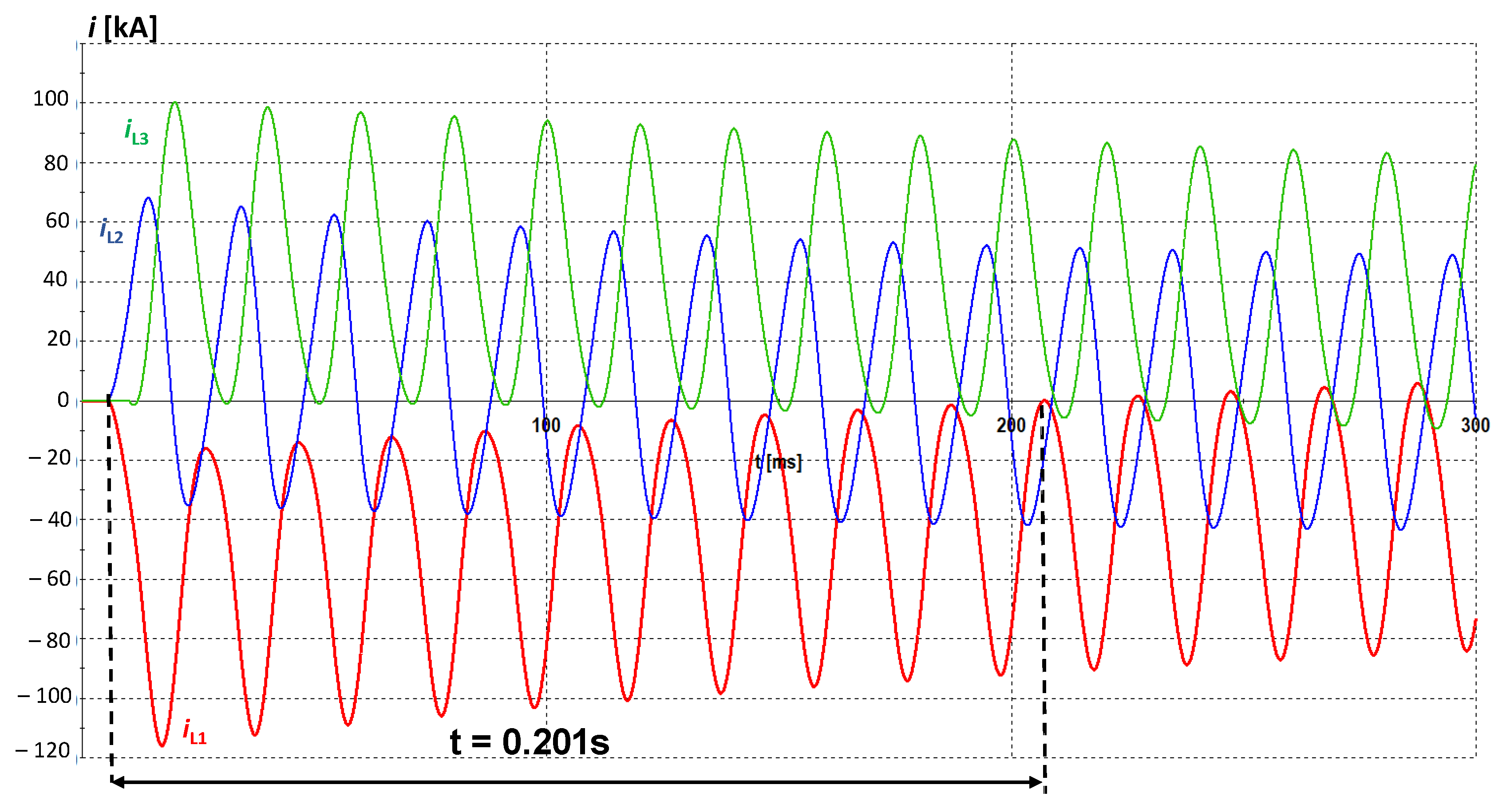
4.2. Delayed Current Zero during Non-Simultaneous Faults

During short-circuit faults, under certain conditions and for the appropriate parameters of the short-circuit circuit, there may be delayed current zeros in individual phases for some time. This phenomenon occurs when the initial value of the DC component is greater than the initial value of the periodic component and/or the subtransient variable components decay faster than the DC component. As it is known, short-circuit currents can only be interrupted under zero-crossing conditions, which means that there may be a situation in which these currents cannot be interrupted for a certain period of time until a natural zero occurs. This phenomenon is therefore directly related to the increase in the value of the DC component contained in the current, which occurs—as shown above—during non-simultaneous faults in relation to the maximum value of this component during simultaneous faults. However, due to the fact that delayed zero currents may also occur during simultaneous short circuits on the generator terminals, these two problems were intentionally separated.
The problem of the delayed current zero during simultaneous three-phase short circuits at generator terminals has been thoroughly analyzed in the literature for a long time [1,5,38,39,40,41]. For this reason, from the point of view of the analysis conducted in this paper, the discussion was limited to examining the impact of the non-simultaneity of faults on this phenomenon.
The main reasons that may cause delayed current zeros during simultaneous short circuits on the generator terminals are the operating conditions before the fault and the parameters of the generator. The influence of the power factor before the fault is important. As it was shown in [41], in the case of a capacitive power factor of generators, the time from the occurrence of the short circuit to the first zero of the short-circuit current is several times longer than in the case of an inductive factor. Delayed current zeros can also be caused by the under-excitation of the generators and the inequality of reactance in both axes of the machine.
The inequality xdxq occurring in machines with salient poles without damping windings may, with the additional consideration of non-simultaneous short circuits, cause the peak factor ksz to reach significant values, and consequently a long time of delayed current zeros. This can be confirmed by the course of the current in the L1 phase during a non-simultaneous three-phase short circuit on the generator terminals for xq″ = 1.5 xd″ (Figure 12).
As it can be noticed, there is a possibility of more than 10 periods of delayed current zeros. These waveforms were computed for extremely unfavorable conditions during which maximum peak factors occur. According to the information provided in Table 1, assuming the zero point of the isolated generator, the most unfavorable case is a non-simultaneous three-phase short circuit, in which, in the first stage, at the moment of a zero of the phase-to-phase voltage of the phases affected by the short circuit (e.g., during a short circuit of phases L1 + L2, this applies to voltage uL1–L2), a two-phase short circuit occurs, and after a delay of 5 ms a three-phase short circuit (when the voltage of the third phase passes through zero).
In practice, three-phase short circuits on the generator terminals are very rare, while the same short circuit—in the above-mentioned extremely unfavorable conditions—due to the “equalizing” reactances xd″ and xq″ causes a much shorter decay time of the zero crossing of short-circuit currents. This is clearly visible in Figure 13, where the waveform of the current in the L1 phase is shown during a non-simultaneous three-phase short circuit at the terminals of the transformers connected to the generator. Therefore, this waveform corresponds to the short-circuit conditions presented in Figure 12, with the location of the fault “shifted” to the secondary side of the transformer when counting from the generator terminals.
In a power system with the specific structure, of a large number of generators in power plants connected by short high-voltage lines, there are favorable conditions for the occurrence of non-simultaneous zero-crossing currents during short circuits.
Additionally, during short circuits distant from the generator terminals, temporary delayed current zeros may occur.
Extreme cases occur when r/x = 0. For x0/x1 = 1, an increase in the peak factor does not occur in reference to the surge factor, which means that the maximum values of the currents during non-simultaneous faults are not greater than those occuring during simultaneous faults and that there is no delayed current zeros.

5. Overvoltages during Non-Simultaneous Faults

5.1. Preliminary Remarks

Knowledge of the phenomena related to switching overvoltages caused by a change in the power system configuration is required both to determine the selection of the parameters of the system insulation protective devices, as well as to select the type and settings of power automatic protection devices. The result is a whole series of publications presenting both measurement results and theoretical analyses containing models of power system elements and calculation methods for testing switching overvoltages [42]. The importance of knowing the quantities characterizing overvoltages, such as peak values and duration, confirms the fact that this research continues, especially in the search for appropriate models and calculation methods [43], despite the fact that these studies have been conducted for over 90 years. Undoubtedly, the main reason for this is the continuous development of computer technology, especially in the direction of the speed and capacity of digital machines. This allows for the use of very accurate line models, which play a fundamental role in these studies, as well as fault models containing nonlinearities.
The influence of individual parameters and system operating conditions on the form, duration and peak values of the overvoltages in the system during simultaneous faults is studied quite well in the literature. However, these relationships cannot be directly transferred to non-simultaneous faults. The combination of short-circuit delays of individual phases or their activation may result in the overlapping of free components and the possibility of the emergence of conditions conducive to the formation of maximum values in each phase. The regularity regarding simultaneous faults, which concerns the occurrence of maximum overvoltages in the phase affected by the short circuit at the time of occurrence of the fault when the voltage of this phase reaches its maximum value, is not always fulfilled during non-simultaneous faults. This is because the free components of the higher frequency add to the value of the basic voltage, meaning that the components’ relative positions can significantly determine the peak value of the resulting voltage.
The numerical analysis of the effect of non-simultaneity on overvoltage factors is much more complicated than when examining this effect on the increase in the peak factor of short-circuit currents. In addition to the non-simultaneity of circuit breaker poles, the possibility of the non-simultaneous closing of circuit breakers at both ends of the line during reclosing in the auto-reclosing cycle should also be taken into account. Current and voltage waveforms during a cycle when circuit breakers operate simultaneously are unlikely.
The analysis of overvoltages during non-simultaneous short circuits and switching faults was conducted for three power systems:
  • Similar to systems operating in the Polish power system (Figure 14);
  • Working in mountain conditions (Figure 15);
  • The system (Figure 16) working in tropical–desert conditions.

5.2. The Influence of the Non-Simultaneity of Faults

In order to assess the impact of the non-simultaneity of faults on the voltage peak values, it is impossible to conduct research whose results would allow for generalizations regarding the delay times of phase short-circuiting, as was the case with the analysis of peak factors of short-circuit currents. This is a direct result of the nature of voltage transient waveforms, which contain an infinite number of free components of higher frequency, determining the voltage peak values. The component amplitudes depend primarily on the moment of the occurrence of the fault and the parameters of the considered system. The frequency of the components occurring in the voltage waveforms of the transmission line depends on the type and the location of the fault. This frequency is inversely proportional to the length of the line. For a very short line, as well as faults located near the measurement point, there is a greater possibility that the maximum values of components with larger pulsations will be added to the amplitudes of the basic voltage. However, these components are attenuated faster in such a line than for one that is longer. This is clearly visible after comparing the voltage waveforms at the beginning of the line with a changed length of 10 and 100 km (Figure 17 and Figure 18, respectively), located as the B-C line in the arrangement shown in Figure 14, where overvoltages appear in all phases when the fundamental components reach voltages of these phases at or near their maximum values. These moments were deliberately chosen as the beginning of the short-circuiting of successive phases during a non-simultaneous three-phase-to-ground short circuit at the end of this line. With the increase in the length of the line, the “required” moment of the short-circuit occurrence is shifted in subsequent phases to achieve the instantaneous maximum value of the voltage transient waveform, which results from the much lower frequency of the components overlapping the basic waveform. The occurrence, even for very short lines, of overvoltages in healthy phases resulting from phase-to-phase couplings is characteristic.
To determine the impact of the non-simultaneity of faults on the voltage peaks during short circuits, simulations were performed, for which the length of the line and the short-circuit power of the substitute power supply systems were modified. As it can be seen from the list shown in Figure 19, in the entire range, the peak voltage values obtained during non-simultaneous short circuits are several to several dozen percent higher than the same values computed during simultaneous short circuits. A percentage increase in the peak voltage values was computed during non-simultaneous and simultaneous faults, regardless of the phase, where the calculation was based on the the ratio of the maximum voltage values evaluated during non-simultaneous and simultaneous faults, regardless of the phase (Figure 19).
Research has shown a vast number of factors influencing the overvoltage factors, and many times the change in individual parameters for a given configuration of the system does not cause a significant change in the values of these factors, but only a change in the “circumstances”, e.g., the time of the voltage peak during the ongoing transient process. For this reason, numerical analysis to determine the delay times of phase short-circuiting and ranges of switching angles, during which maximum overvoltages may occur, is very tedious and time-consuming. This is probably the reason why the phenomenon of non-simultaneity of faults is completely ignored in numerous studies of transients, which comprehensively analyze the influence of many factors of much lesser, sometimes even negligible, importance [44]. This is all the more surprising as numerous studies devote considerable space to the analysis of fault models, under the erroneous assumption of its simultaneous occurrence.
Table 3 lists the overvoltage factors that were computed at the beginning of the analyzed line during simultaneous and non-simultaneous, switching and short-circuit faults. Three characteristic types of interference were selected:
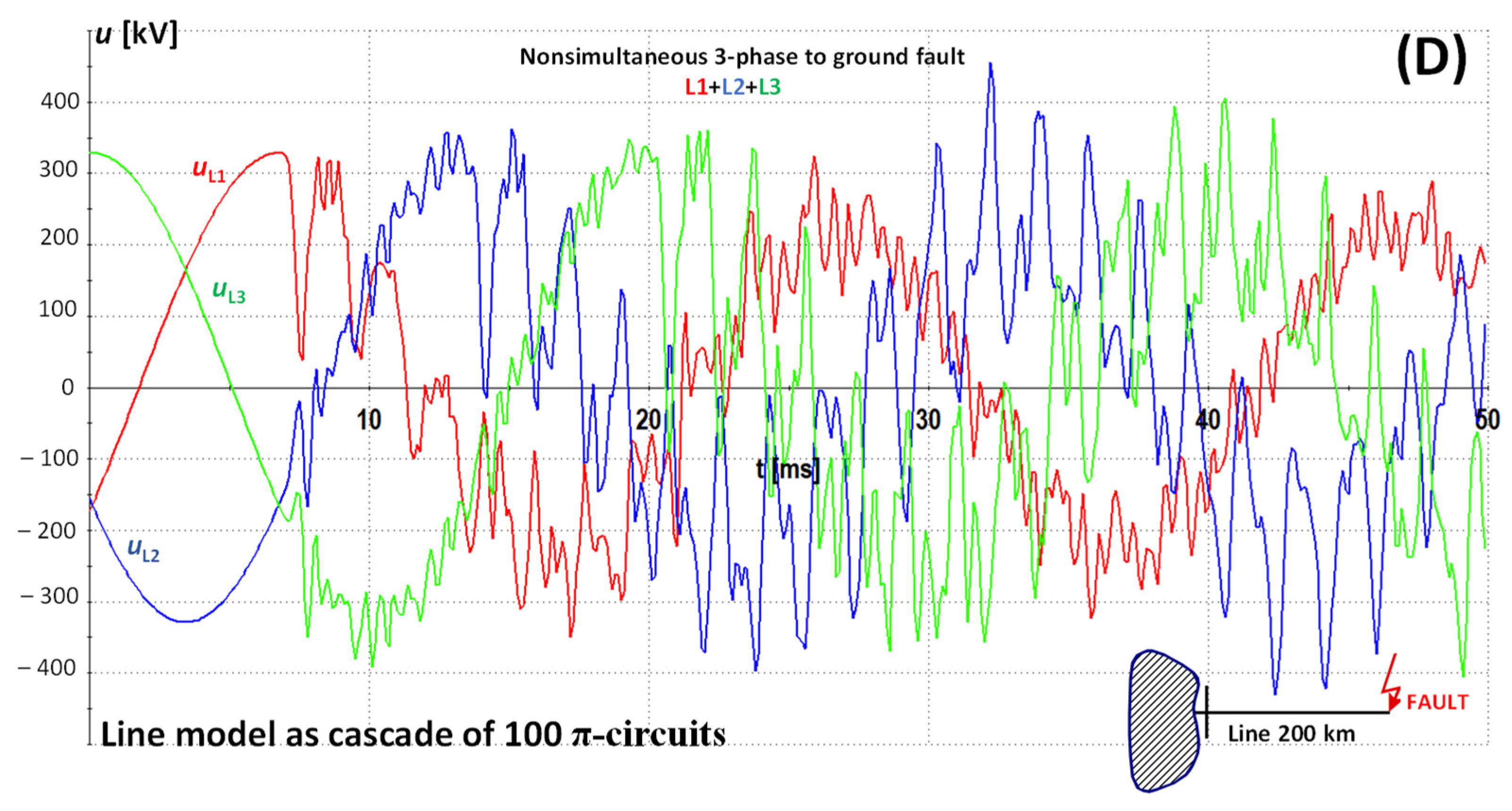
  • Non-simultaneous three-phase-to-ground short circuits at the end of the line;
  • Three-phase reconnection of the line (non-simultaneous and simultaneous on both sides) after the elimination of the fault;
  • Three-phase reconnection of the line (non-simultaneous and simultaneous on both sides) with a permanent single-phase short circuit.
The latter type of faults is the most dangerous case, which can be confirmed judging by the values of the overvoltage factors presented in the table, while the influence of the length of the transmission line on the factors calculated is not clear. As for the external conditions of the system set in the presented example, such as configuration, the short-circuit power of the power supply systems and parameters, an occurrence of the highest values of the maximum overvoltage factors can be noticed for the 70 km long line.
This analysis and its results clearly indicate the need for the consideration of the actual state of short-circuit and switching faults, which is the non-simultaneous occurrence of the fault in each of the phases.
Among the other factors influencing the values of the overvoltage factors, independent of taking into account the non-simultaneous occurrence of faults, local and general phenomena should be distinguished. Local factors specific to a particular system, which determine the general level of overvoltage factors that may occur in this system, are deterministic. These include:
  • Parameters and the structure of the system. The parameters of the transmission lines play a fundamental role, but also those of power supply systems, mainly the mutual impedance ratio for a zero and positive sequence as well as the resistance and reactance;
  • The influence of the line load and system operating conditions (in a normal state) before the fault is negligible.
The general factors of a probabilistic nature are:
Type of fault. This applies to possible ground involvement during a short circuit.
As shown above for non-ground short circuits, the free higher frequency components causing overvoltages appear practically only in the phases affected by the short circuit, in contrast to ground faults, during which the amplitudes of the components in the healthy phases may be larger than in the phases affected by the fault.
Distance from the fault site. It is a factor indirectly related to the local parameter, which is the length of the line. The time during which a fault wave “needs” to travel from the location of the fault to the first point of discontinuity, causing the reflection of this wave, determines the frequency of the components, their amplitude and the damping time.
The moment of the short-circuit. The maximum amplitudes of the free components occur for a fault in the phase whose voltage at the short-circuit site reaches its maximum value at the time of the short-circuit occurrence. The non-simultaneous occurrence of a short circuit may cause this statement to be false. For example, in a short-circuited phase, there may be components with a significant amplitude at the moment when the voltage of this phase passes through zero (for a simultaneous short circuit, there are no components in such conditions).
Multiple reflections of waves at nodal points cause the transient appearance of free components of a higher frequency in the waveforms of instantaneous voltages and currents. These components can be easily recorded at the ends of the line during faults. In the past, there was an idea to use these components in algorithms for fast line protection and short-circuit locators [45]. This trend was abandoned due to many factors that could cause the faulty operation of the protection devices and locators based on the measurement of these components.
This is because the superimposition of reflected surge waves in multi-wire systems causes an overvoltage phenomenon that may cause unnecessary action of protections.
It seems that, in the near future, perfected, verified computational tools [46] should be used to study non-simultaneous faults, omitted for incomprehensible reasons.
The range of comparisons of the results of numerical tests with the results of short-circuit tests is small, which is an obvious consequence of the very small number of descriptions of tests in real power systems available in the national and international literature. Such research—as is known—is very rare for economic, technical and organizational reasons. For this reason, any publication presenting a comparison of the results of theoretical and measurement studies is very desirable [47].

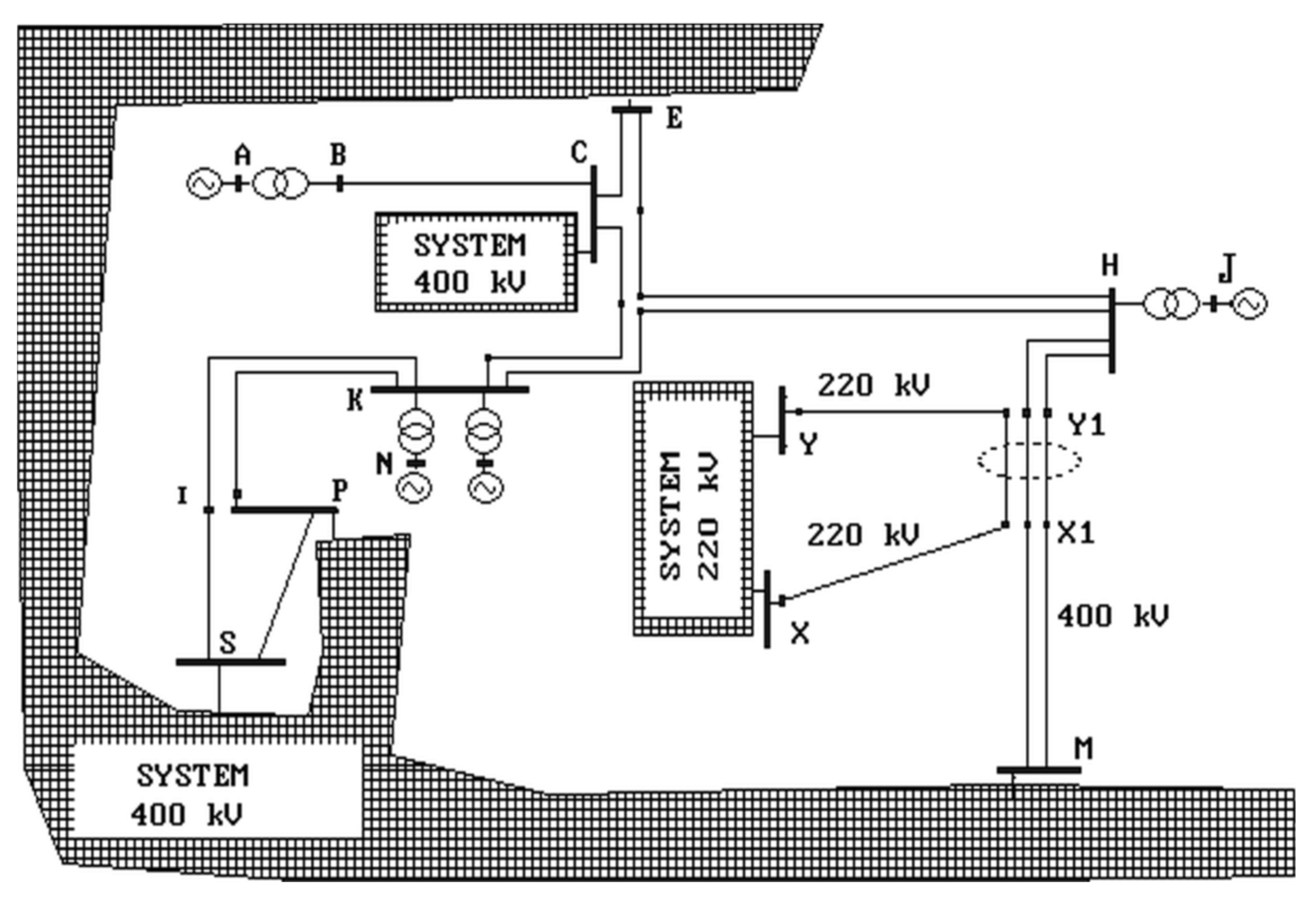
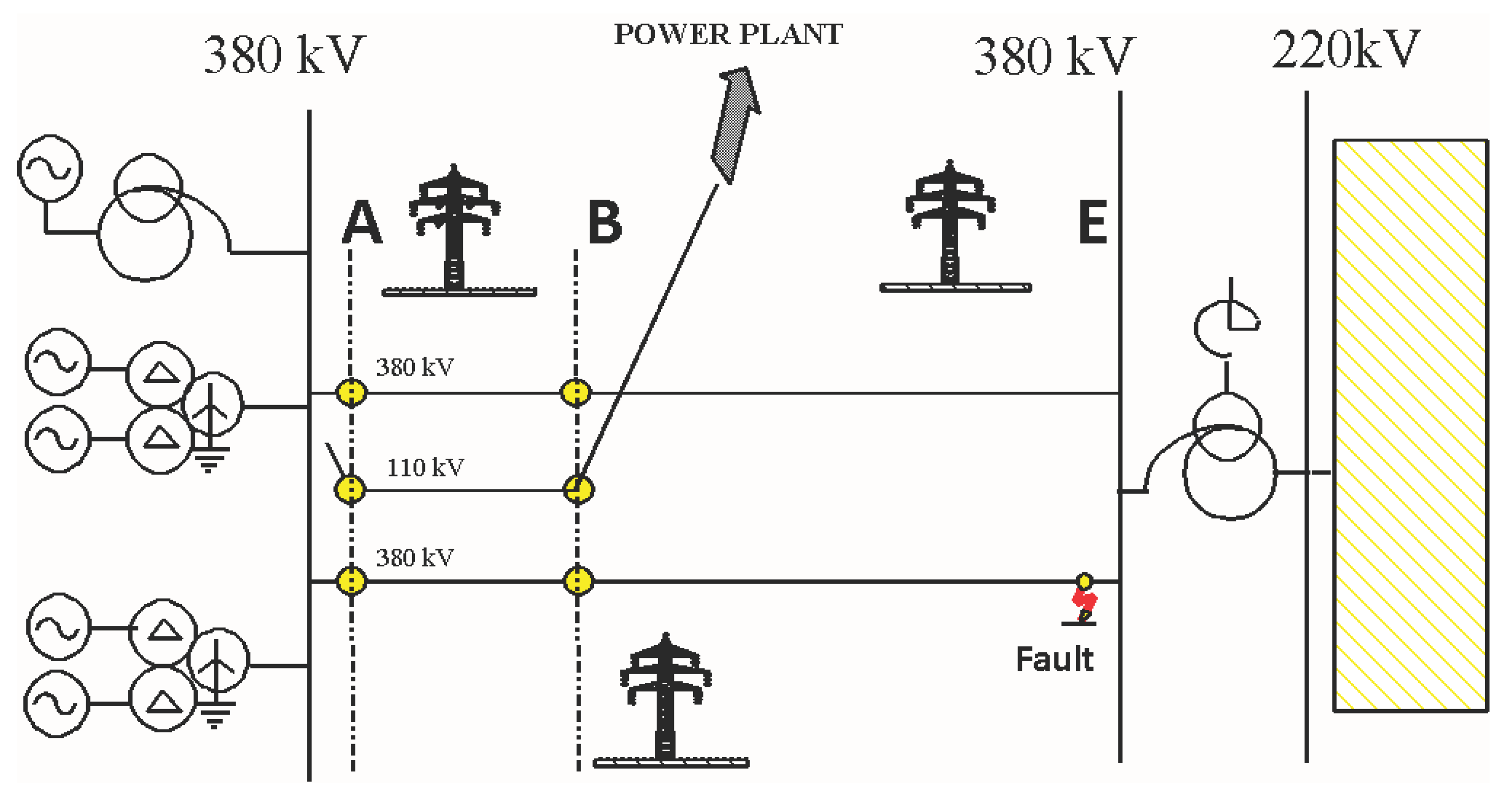
6. Overvoltages in Transmission Lines with Different Voltage Levels Operating on the Same Supporting Structures

The phenomenon of overvoltages in the adjacent conductors of the line has been analyzed in the literature quite thoroughly; so, additional research will not add significant innovations regarding the results of possible calculations. However, this conclusion can only be applied to multi-conductor lines with the same voltage level, operating in the same system, in most cases connected to common busbars.
In contrast, the problem of transient phenomena that may occur in lines without faults, as a consequence of short circuits appearing in other tracks operating on the same supporting structure, but with different voltage levels, has to date been considered only fragmentarily. These phenomena can lead to unnecessary cascading shutdowns of lines that are in a faultless state. In addition, due to the fact that these conductors are connected to different systems, the location of these faults and their elimination may be very difficult.
The analysis of this problem was conducted on the basis of the calculation results obtained for the system operating in mountain conditions, used in the verification analysis (Figure 15). The 110 kV transmission line was suspended on the same support poles as the 380 kV line in the 13 km section.
As the tests showed, the highest instantaneous voltage values were obtained in both lines during a non-simultaneous three-phase-to-ground short circuit. The calculations show the presence of significant values of instantaneous voltages in a 110 kV line, which was not affected by the fault during non-simultaneous short circuits in a 380 kV line. Table 4 shows the maximum overvoltage factors in both tested lines, defined as the multiplicity of the peak phase voltage during selected short-circuit faults in the 380 kV line.
The presented factors are obviously not the maximum possible ones, due to the fact that higher values may occur during faults of a different type (e.g., switching) or in a different location. The operating conditions of the 110 kV line are also very important. At the time of the measurements on the 380 kV line, the 110 kV line was not yet connected to any system. The list presented in the table concerns the expected structure and operating conditions of the 110 kV network to which this line was to be connected.
The examples of voltage transients shown in Figure 20 were calculated at the beginning of the 110 kV line during a three-phase non-simultaneous short circuit at the end of the 380 kV line, for the current condition, i.e., when the 110 kV line was not connected to any system. As it can be noticed, despite this, voltages exceeding the rated value appear in this line due to coupling.
The voltage waveforms shown in Figure 20 were calculated for a 110 kV line connected to the power supply at one side, without a load. The consequence of this is that very-high overvoltage factors appeared during the same short circuit. The instantaneous voltage in the L3 phase reaches a value almost 3.5 times higher than the rated voltage.
A very dangerous, albeit extremely rare, fault that may cause overvoltages in neighboring systems is the breaking of a ground wire or a phase wire. As a result, inter-system multiphase ground faults or non-ground faults may occur. It is very important that during such faults—especially in lines with a lower voltage level—short-circuit currents of much higher values occur compared to the currents flowing during short circuits in one system. Example waveforms are shown in Figure 21.

7. Concluding Remarks

Extremely different conditions for the occurrence of maximum transient voltages and currents (maximum overvoltages for the moment of the initial fault, when the voltage of the phase affected by the short-circuit reaches its maximum, and the maximum peak current, when the voltage crosses zero in the short-circuited phase at the time of the occurrence of the short circuit) imply that, practically always during faults, free components with various damping times and amplitudes appear. Taking into account the phenomenon of the overlapping of these components during non-simultaneous faults, there is a problem of the increase in these damping times and amplitudes in reference to the values calculated for simultaneous faults.
A significant problem is also the fact that the standards accept the results of calculations conducted for simultaneous faults. This applies primarily to the possibility of exceeding the value of the maximum surge current for simultaneous short circuits, adopted in the standards as the maximum for all types of faults with ku = 2, as well as delayed current zeros.
As the results of the research presented above show, there is a wide range of possible conditions conducive to the emergence of such situations.
The non-simultaneity of short circuits and switching faults causes a significant increase in overvoltage factors in relation to the maximum ones calculated during these faults treated as simultaneous.
The possibilities of overvoltages in lines with different voltage levels, connected to different systems, but operating on the same supporting structures, are of particular practical importance. It was shown that non-simultaneous short circuits in adjacent lines can cause high-amplitude overvoltages. As a consequence, triggered protections in these adjacent conductors may incorrectly disconnect these lines. By cascading down successive lines, a “blackout” may even occur.
The above-mentioned common opinions expressed in the international and domestic literature about the low probability of conditions conducive to the occurrence of increased short-circuit currents during non-simultaneous faults do not justify such an “optimistic” approach to the increase in possible overvoltage factors. Overlapping free high-frequency components cause the distortion of the voltage waveform, the amplitude of which depends on a vast number of parameters and conditions prevailing in the system during the fault. Therefore, it is not possible to formalize the ranges, for which overvoltage factors during non-simultaneous short circuits increase or decrease in relation to simultaneous faults. As shown by the test results shown above, the increase in overvoltage rates occurs for a very wide range of phase shorting delays, as well as for many combinations of non-simultaneous faults.

Author Contributions

P.S. and D.Z. contributed equally to this work, in all of its stages and elements. All authors have read and agreed to the published version of the manuscript.

Funding

This research received no external funding.

Data Availability Statement

No new data were created or analyzed in this study. Data sharing is not applicable to this article.

Conflicts of Interest

The authors declare no conflict of interest.

References

  1. Oswald, B.; Siegmund, D. Berechnung von Ausgleichsvorgängen in Elektroenergiesystemen; Deutscher Verlag für Grundstoffindustrie: Leipzig, Germany, 1991. [Google Scholar]
  2. Canay, M.; Werren, L. Interrupting sudden asymmetric short-circuit current without zero transition. Brown Boveri Rev. 1969, 56, 484–493. [Google Scholar]
  3. Canay, M.; Klein, H. Asymmetric short-circuit currents from generators and the effect of the breaking arc. Brown Boveri Rev. 1974, 61, 199–206. [Google Scholar]
  4. Owen, R.E.; Lewis, W.A. Asymmetry characteristics of progressive short-circuits on large synchronous generators. IEEE Trans. Power Appar. Syst. 1971, PAS-90, 587–596. [Google Scholar] [CrossRef]
  5. Kulicke, B.; Schramm, H.H. Clearance of Short-Circuits with Delayed Current Zeros in the ITAIPU 550 kV-Substation. IEEE Trans. Power Appar. Syst. 1980, PAS-99, 1406–1414. [Google Scholar] [CrossRef]
  6. Lim, L.S.; Smith, I.R. Turbogenerator shirt circuits with delayed current zeros. Proc. Inst. Electr. Eng. 1977, 124, 1163–1169. [Google Scholar] [CrossRef]
  7. Bogucki, A.; Sowa, P. Transiente Vorgänge während Kurzschlußfolgefehlern in Elektroenergiesystemen. In Proceedings of the 10. Wiss. Konf. der Sektion Elektrotechnik der TU Dresden, Dresden, Germany, 10–12 July 1984; pp. 45–49. [Google Scholar]
  8. Bogucki, A.; Sowa, P. Ströme und Kräfte bei kurzschlußartigen Folgefehlern. In Proceedings of the 31. Int. Wiss. Kolloquium, Ilmenau, H1, Ilmenau, Germany, 27–31 October 1986; pp. 7–10. [Google Scholar]
  9. Nordman, H. Current and forces in non-simultaneous three-phase short circuits. Sähkö 1974, 47, 82–86. [Google Scholar]
  10. Tsanakas, D. Ströme, Kräfte und mechanische Beanspruchung bei nicht gleichzeitig eintretenden Kurzschlüssen. etz-a 1975, 96, 501–505. [Google Scholar]
  11. Goto, M.; Nohara, H.; Takahashi, I.; Watanabe, A.; Kawai, T. Delayed Current-Zero Phenomena Caused by Transmission Line Faults. Trans. Inst. Electr. Eng. Jpn. B 1986, 106, 701–708. [Google Scholar] [CrossRef]
  12. Sowa, P.; Zychma, D. Dynamic Equivalents in Power System Studies: A Review. Energies 2022, 15, 1396. [Google Scholar] [CrossRef]
  13. Kulicke, B. Simulationsprogram Netomac: Differenzen-Leitwertverfahren bei kontinuierlichen und diskontinuierlichen Systemen. Siemens Forsch.-Und Entwickl. Ber Bd. 1981, 10, 299–302. [Google Scholar]
  14. Mahseredjian, J.; Dinavahi, V.; Martinez, J.A. Simulation Tools for Electromagnetic Transients in Power Systems: Overview and Challenges. IEEE Trans. Power Deliv. 2009, 24, 657–1669. [Google Scholar] [CrossRef]
  15. Ametani, A. Electromagnetic transients program: History and future. IEEJ Trans. Electr. Electron. Eng. 2021, 16, 1150–1158. [Google Scholar] [CrossRef]
  16. European EMTP User Group. ATP Rule Book; EEUG: Offenbach, Germany, 2007. [Google Scholar]
  17. Mahseredjian, J.; Dennetiere, S.; Dube, L.; Khodabakhchian, B.; Gerin-Lajoie, L. On a new approach for the simulation of transients in power systems. Electr. Power Syst. Res. 2007, 77, 1514–1520. [Google Scholar] [CrossRef]
  18. Dommel, H.W. EMTP Theory Book; Microtran Power System Analysis Corp: Vancouver, BC, Canada, 1992. [Google Scholar]
  19. Marti, J.R. Accurate modeling of frequency-dependent transmission lines in electromagnetic transient simulations. IEEE Trans. Power Appar. Syst. 1982, 101, 147–155. [Google Scholar] [CrossRef]
  20. Kocar, I.; Mahseredjian, J.; Olivier, G. Improvement of Numerical Stability for the Computation of Transients in Lines and Cables. IEEE Trans. Power Deliv. 2010, 25, 1104–1111. [Google Scholar] [CrossRef]
  21. Noda, T.; Nagaoka, H.; Ametani, A. Phase domain modeling of frequency-dependent transmission lines by means of an ARMA model. IEEE Trans. Power Deliv. 1996, 11, 401–411. [Google Scholar] [CrossRef]
  22. Castellanos, F.; Marti, J.R. Full frequency-dependent phase-domain transmission line model. IEEE Trans. Power Syst. 1997, 12, 1331–1339. [Google Scholar] [CrossRef]
  23. Carson, J.R. Wave propagation in overhead wires with ground return. Bell Syst. Tech. J. 1926, 5, 539–554. [Google Scholar] [CrossRef]
  24. Deri, A.; Tevan, G.; Semlyen, A.; Castanheira, A. The complex ground return plane, a simplified model for homogenoeous and multi-layer earth return. IEEE Trans. Power Appar. Syst. 1981, PAS-100, 3686–3693. [Google Scholar] [CrossRef]
  25. Siegmund, D.; Sowa, P. Zur Modellierung von Elektroenergieübertragungsleitungen mit konzentrierten Parametern―ein Vergleich zwischen digitaler und analoger Simulation. Wiss. Z. Der Tech. Univ. Dresd. 1987, 36, 97–102. [Google Scholar]
  26. Tavares, M.C.; Pissolato, J.; Portela, C.M. New multiphase mode domain transmission line model. Int. J. Electr. Power Energy Syst. 1999, 21, 585–601. [Google Scholar] [CrossRef]
  27. Jalali, F. Transmission Line Experiments at Low Cost. In Proceedings of the 1998 ASEE Annual Conference, Seattle, WA, USA, 28 June–1 July 1998. [Google Scholar]
  28. Portela, C.M.; Tavares, M.C. Six-Phase Transmission Line-Propagation Characteristics and New Three-Phase Representation. IEEE Trans. Power Deliv. 1993, 8, 1470–1482. [Google Scholar] [CrossRef]
  29. Carneiro, S.; Marti, J.R. Evaluation of corona and line models in electromagnetic transients simulations. IEEE Trans. Power Deliv. 1991, 6, 334–342. [Google Scholar] [CrossRef]
  30. Ishii, M.; Kawamura, T.; Kouno, T.; Ohsaki, E.; Shiokawa, K.; Murotani, K.; Higuchi, T. Multistory transmission tower model for lightning surge analysis. IEEE Trans. Power Deliv. 1991, 6, 1327–1335. [Google Scholar] [CrossRef]
  31. Bogucki, A.; Sowa, P. Transient Caused by Non-Simultaneous Arcing Faults. In Proceedings of the Sixth International Symposium on High Voltage Engineering, New Orleans, LA, USA, 28 August–1 September 1989. [Google Scholar]
  32. Cornick, K.J.; Ko, Y.M.; Pek, B. Power system transients caused by arcing faults. IEE Proc. C 1981, 128, 18–27. [Google Scholar] [CrossRef]
  33. Johns, T.; Al-Rawi, A.M. Digital Simulation of EHV systems under secondary arcing conditions associated with single-pole autoreclosure. IEE Proc. C 1982, 129, 49–58. [Google Scholar] [CrossRef]
  34. Hoseman, G. Berechnung der Kurzschlußströme und -kräfte in der Normung. etz-a 1976, 97, 298–303. [Google Scholar]
  35. IEC 60909-0:2016; Short-Circuit Currents in Three-Phase a.c. Systems–Part 0: Calculation of Currents. International Electrotechnical Commission: Geneva, Switzerland, 2016; ISBN 978-2-8322-3158-6.
  36. Błaszczyk, A.; Popczyk, J. Auswahl von 110-kV-Schaltern auf der Basis eines probabilistischen Modells. ELEKTRIE 1983, 5, 242–245. [Google Scholar]
  37. Ciok, Z. Non-simultaneous short-circuits in three-phase networks with special consideration to the effect upon operation of circuit-breakers. In Proceedings of the CIGRE, Paris, France, 16–26 May 1962. [Google Scholar]
  38. Hernandes, L.; Marques, F.Z.; Vasconcellos, A.S. Delayed current zeros in FPSO offshore units. In Proceedings of the 2014 IEEE Petroleum and Chemical Industry Conference—Brasil (PCIC Brasil), Rio de Janeiro, Brazil, 25–27 August 2014; pp. 147–154. [Google Scholar] [CrossRef]
  39. Eidinger, A. Interniption of high asymmetric short- circuit currents having long delayed zeros—An acute problem for generator breakers. IEEE Trans. PAS 1972, 91, 1725–1731. [Google Scholar]
  40. Braun, D.; Köppl, G.S. Transient Recovery Voltages During the Switching Under Out-of-Phase Conditions. In Proceedings of the International Conference on Power Systems Transients—IPST 2003, New Orleans, LA, USA, 28 September–2 October 2003. [Google Scholar]
  41. Vajnar, V.; Vostracky, Z. Reduced breaking capability of circuit breakers within operations with delayed current zeros. In Proceedings of the 2016 17th International Scientific Conference on Electric Power Engineering (EPE), Prague, Czech Republic, 16–18 May 2016; pp. 1–5. [Google Scholar]
  42. Ciok, Z. Einschwingspannung nach Abstandskurzschlüssen. ELEKTRIE 1981, 10, 552–553. [Google Scholar]
  43. Working Group 02 of Study Commitee 33. Guidelines for representation of network elements when calculating transients. CIGRE-Broch. 1990, 39. [Google Scholar]
  44. Johns, T.; Aggarwal, R.K. Digital simulation of faulted e.h.v. transmission lines with particular reference to very high-speed protection. Proc. Inst. Electr. Eng. 1976, 123, 353–359. [Google Scholar] [CrossRef]
  45. Boonybol, C. Power Transmission System Fault Simulation Analysis and Location. Ph.D. Thesis, University of Missouri, Columbia, MO, USA, 1968. [Google Scholar]
  46. Mahseredjian, J. Computation of power system transients: Overview and challenges. In Proceedings of the 2007 IEEE Power Engineering Society General Meeting, Tampa, FL, USA, 24–28 June 2007. [Google Scholar] [CrossRef]
  47. Cervantes, M.; Ametani, A.; Martin, C.; Kocar, I.; Montenegro, A.; Goldsworthy, D.; Tobin, T.; Mahseredjian, J.; Ramos, R.; Marti, J.R.; et al. Simulation of Switching Overvoltages and Validation with Field Tests. IEEE Trans. Power Deliv. 2018, 33, 2884–2893. [Google Scholar] [CrossRef]
Figure 1. Frequency-dependent line model representation.
Energies 16 06618 g001
Figure 2. Comparison of the transient waveforms for the different numbers of applied π-circuits.
Energies 16 06618 g002
Figure 3. Comparison of transients by the different line model. (A) 10 km line by JMarti model, (B) 10 km line modeled as cascade of 100 π-circuit, (C) 200 km line by JMarti model, (D) 200 km line modeled as cascade of 100 π-circuit.
Energies 16 06618 g003aEnergies 16 06618 g003b
Figure 4. Comparison of voltage waveforms at the beginning of the line calculated in the network with the distributed line parameters—constant and frequency-dependent line parameters.
Energies 16 06618 g004
Figure 5. Multistory transmission tower model [30].
Energies 16 06618 g005
Figure 6. General classification of transients according to the time range and frequency of the components.
Energies 16 06618 g006
Figure 7. Factors of the peak current kszL1 during the non-simultaneous three-phase-to-ground fault for x0/x1 = 0.5, r/x = 0.07.
Energies 16 06618 g007
Figure 8. Factors of the peak current kszL1 during the non-simultaneous three-phase-to-ground fault for x0/x1 = 10, r/x = 0.07.
Energies 16 06618 g008
Figure 9. Factors kszL1 of the peak current during the non-simultaneous three-phase-to-ground fault.
Energies 16 06618 g009
Figure 10. Factors kszL1 and kszL1 of peak currents during the non-simultaneous two-phase-to-ground fault.
Energies 16 06618 g010
Figure 11. Time delay ranges of the faulted phases (factors of peak currents higher than ksz = 2).
Energies 16 06618 g011
Figure 12. Current waveform during a non-simultaneous three-phase fault at the terminals of a synchronous generator for xq″ = 1.5 xd″.
Energies 16 06618 g012
Figure 13. Current waveform in phase L1 during a non-simultaneous three-phase fault at the transformer terminals.
Energies 16 06618 g013
Figure 14. Part of Polish test system.
Energies 16 06618 g014
Figure 15. Test system working in mountain conditions.
Energies 16 06618 g015
Figure 16. Test system working in desert conditions.
Energies 16 06618 g016
Figure 17. Voltage waveforms during a non-simultaneous three-phase fault at the beginning of a 10 km line.
Energies 16 06618 g017
Figure 18. Voltage waveforms during a non-simultaneous three-phase fault at the beginning of a 100 km line.
Energies 16 06618 g018
Figure 19. Percentage increase in the voltage peak values during non-simultaneous faults.
Energies 16 06618 g019
Figure 20. Voltage waveforms in the disconnected 110 kV line working on the same tower construction as the faulted 380 kV line during the three-phase non-simultaneous short circuit.
Energies 16 06618 g020
Figure 21. Intersystem fault. (A) Transient voltages in both system, (B) enlarged fragment of transient voltages in the figure (A), (C) transient current during intersystem ffault.
Energies 16 06618 g021aEnergies 16 06618 g021b
Table 1. Symbols and subscripts used in the paper.
ParameterDefinition
S″sc = √3 UnI″scThe (IEC standard [35]) short-circuit power
kuFactor for the calculation of the peak short-circuit current by a simultaneous fault
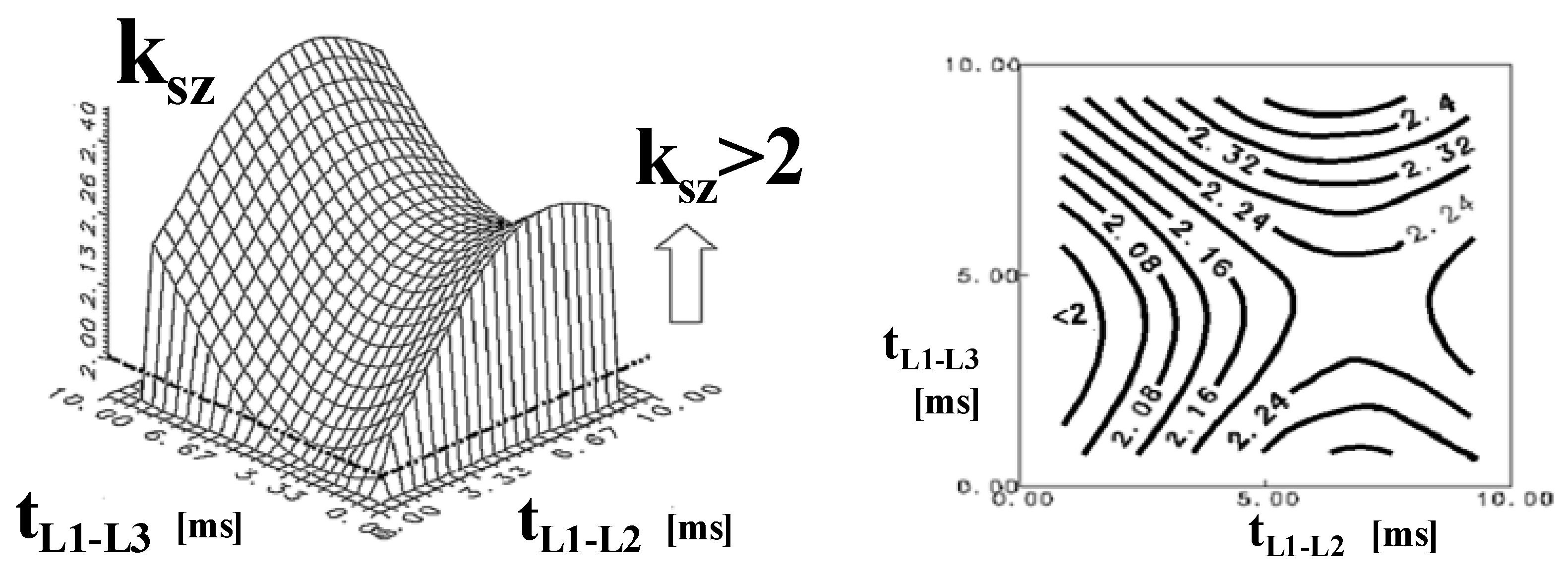
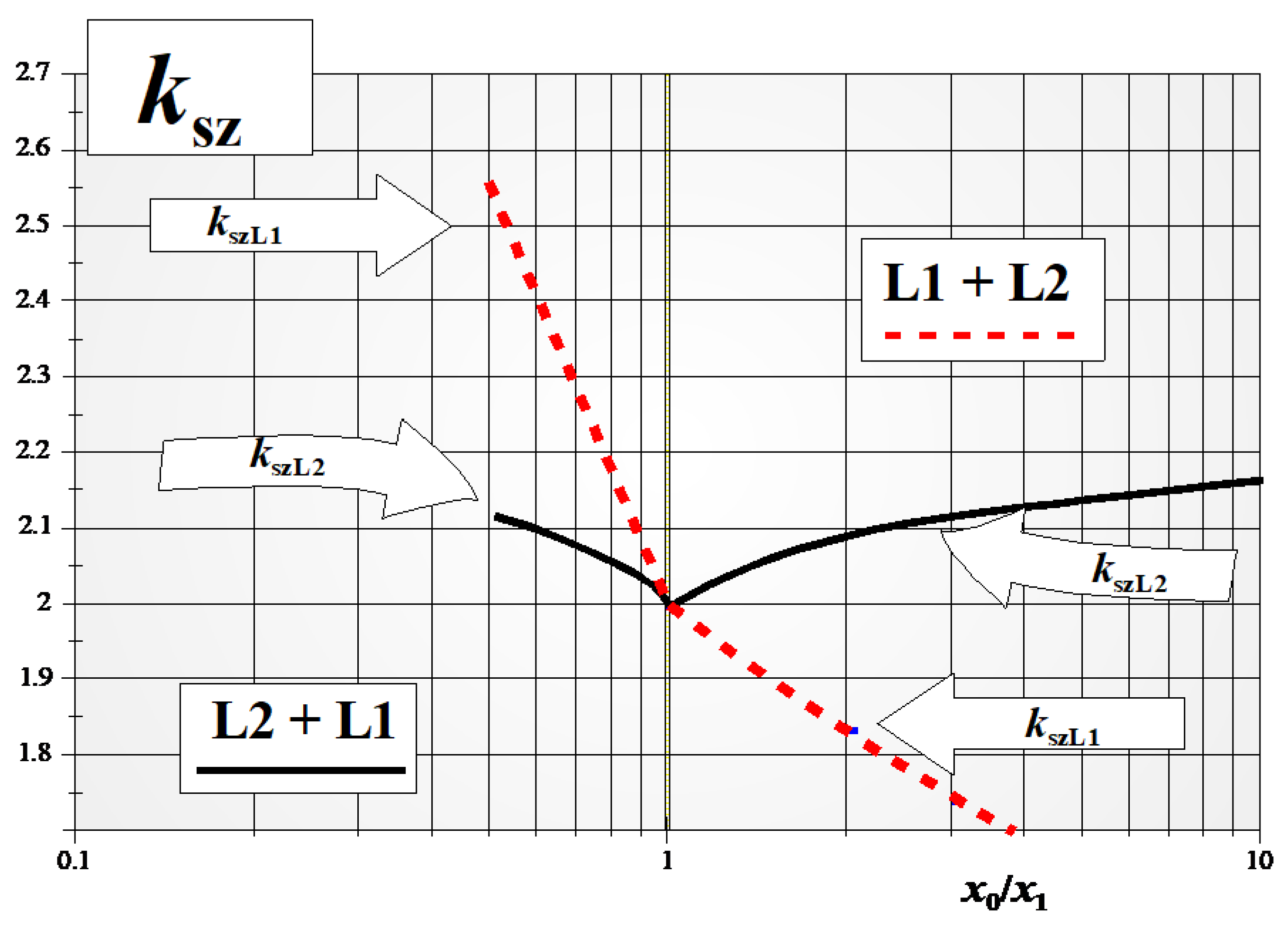
kszThe ratio of the peak current occurring in the case of a non-simultaneous fault to the amplitude of the periodic component at the time of the short circuit
r0Zero-sequence resistance
r1Positive-sequence resistance
x0Zero-sequence reactance
x1Positive-sequence reactance
xdSubtransient reactance of a synchronous machine, direct axis
xqSubtransient reactance of a synchronous machine, quadrature axis
Table 2. List of parameters and their values determining the increase in the peak current value during non-simultaneous short circuits.
ParameterValueNotes
The phase angle of the voltage at the time of the short circuit0Applies to all phases affected by the fault during a three-phase three-stage fault or a two-phase-to-ground fault and phases short-circuited separately during a three-phase two-stage fault for values x0/x1 < 1
applies to phase-to-phase voltage during a three-phase two-stage short circuit for phases shorted simultaneously for the value x0/x1 > 1
Delay time for short-circuiting subsequent phases during a non-simultaneous two-phase short-circuit to earth1.66 ÷ 5 msFor x0/x1 > 1 and L2 + L1 short-circuit order
5 ÷ 6.6 msFor x0/x1 < 1 and L1 + L2 short-circuit order
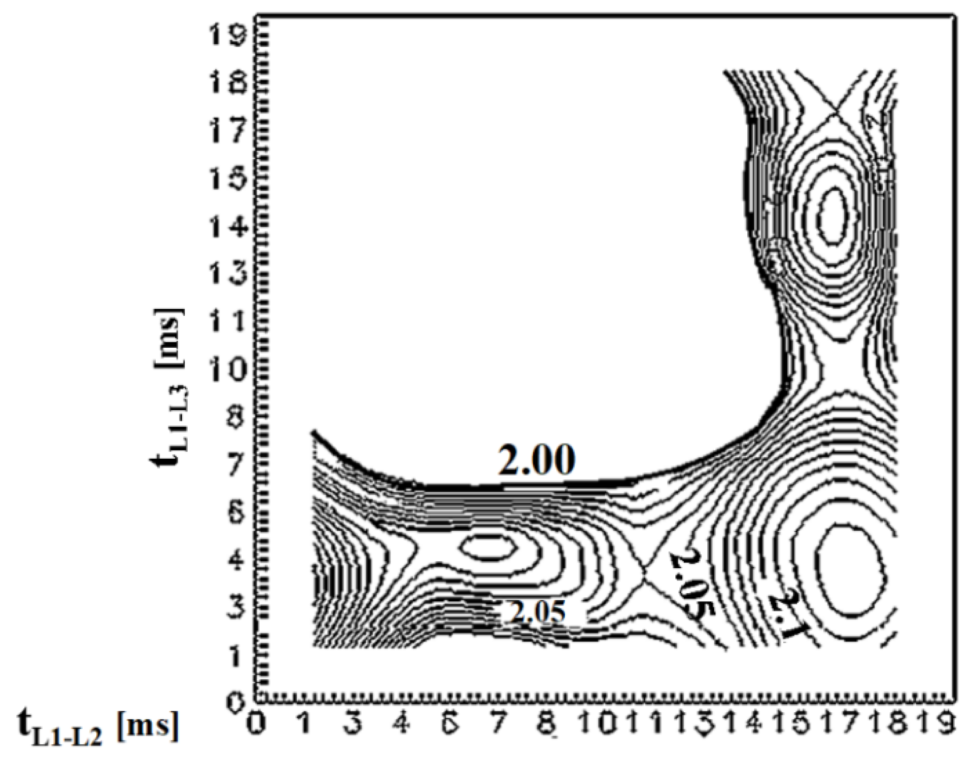
Delay time of successively phased short circuits during a non-simultaneous three-phase-to-ground short circuit≤6.6 msFor x0/x1 < 1 and three-phase two-stage short circuit
≤5 msFor x0/x1 > 1 and three-phase two-stage short circuit
r/x0Theoretically; in practice, the smallest value is 0.07
Table 3. Overvoltage factors during non-simultaneous faults.
Type of FaultThree-Phase-to-Ground Short CircuitSuccessful 3-Phase ReconnectionSuccessful 3-Phase Reconnection with a Permanent Single-Phase Short Circuit
Line Length (km)SimultaneousNon-SimultaneousSimultaneousNon-SimultaneousSimultaneousNon-Simultaneous
101.021.691.691.691.691.69
301.031.761.761.761.761.76
501.081.711.711.711.711.71
701.162.022.022.022.022.02
1001.251.901.901.901.901.90
2501.322.211.332.171.122.23
Table 4. Overvoltage factors during short circuits at the end of a 380 kV line.
Line
(kV)
Type of Short CircuitL1 PhaseL2 PhaseL3 Phase
110L1 + g2.721.881.83
L1 + L21.811.671.91
L1 + L2 + g2.721.902.03
L1 + L2 + L3 (simultaneous)1.491.271.68
380L1 + L2 + L3 + g (non-simultaneous)2.721.902.19
L1 + g1.061.051.14
L1 + L21.341.441.09
L1 + L2 + g1.051.051.14
Disclaimer/Publisher’s Note: The statements, opinions and data contained in all publications are solely those of the individual author(s) and contributor(s) and not of MDPI and/or the editor(s). MDPI and/or the editor(s) disclaim responsibility for any injury to people or property resulting from any ideas, methods, instructions or products referred to in the content.

