Article

Fluid–Structure Interaction Analysis of a Wind Turbine Blade with Passive Control by Bend–Twist Coupling

by
Jorge Mario Tamayo-Avendaño
1,
Ivan David Patiño-Arcila
2,
César Nieto-Londoño
1,3 and
Julián Sierra-Pérez
1,*
1
Grupo de Investigación en Ingeniería Aeroespacial, Universidad Pontificia Bolivariana, Medellín 050031, Colombia
2
Grupo de Investigación e Innovación Ambiental (GIIAM), Institución Universitaria Pascual Bravo, Medellín 050034, Colombia
3
Grupo de Energía y Termodinámica, Universidad Pontificia Bolivariana, Medellín 050031, Colombia
*
Author to whom correspondence should be addressed.
Energies 2023, 16(18), 6619; https://doi.org/10.3390/en16186619
Submission received: 26 July 2023 / Revised: 11 August 2023 / Accepted: 18 August 2023 / Published: 14 September 2023
(This article belongs to the Special Issue Advanced Structural Response and Performance of Wind Turbines)

Abstract

:
The idea of improving the energy output for small wind turbines without compromising the remaining aspects of the technology, such as costs and structural integrity, is very appealing in the context of the growing concern for global warming and the goal of providing electricity to remote and isolated regions. This work aims to contribute to the development of distributed wind generation by exploring the effects of bend–twist coupling on the performance of a wind turbine with a focus on a small rotor based on the NREL Phase VI blade geometry. After defining a structure in composite materials exhibiting the coupling behavior along with a reference counterpart, a comparative numerical analysis is performed using a Fluid–Structure Interaction (FSI) analysis. The main numerical framework is based on commercial software and consists of a finite-volume solver for fluid physics, a finite-element solver for solid physics, and a coupling interface for the interaction problem. The results, complemented with the predictions from a one-way analysis based on the blade-element momentum theory are used to define the increments in rotor torque. The analysis of the annual energy yield shows a 3% increase due to the bend–twist coupling used as a passive pitch mechanism, considering a Rayleigh distribution with an 11 m/s average wind speed. Simultaneously, the coupling causes increments of 0.2% and 0.3% for the blade root flapwise moment and the rotor thrust force, respectively, when considering parked conditions and a simplified extreme wind model.

1. Introduction

In the context of global warming, modern societies are striving to move from fossil fuels towards cleaner renewable energies. Wind energy stands among the top drivers of this transition, and has become widely used in large-scale generation projects and to some extent in small-scale projects. At the same time, the costs of generation from non-conventional renewable sources, including wind and photovoltaic cells, have shown significant reductions over recent years [1]. In modern scenarios, the economic viability of wind energy for small projects, specifically for distributed generation, can be closely contested by competing sources such as photovoltaic or even diesel plants, which in many places can be more accessible and, therefore, more attractive for investors and developers. Current levelized costs of electricity (LCOE) for small applications are still higher than for any other size of wind generation projects [2]; in addition, with the significant reduction in photovoltaic generation costs [1], the question of how to make wind energy competitive compared to other technologies arises.
Economic feasibility can be achieved if the energy output represented by the Annual Energy Production (AEP) is improved without compromising capital and operation costs. This is consistent with the LCOE definition and hints at how innovation must advance to strengthen the position of wind energy among other non-conventional renewable energy sources. Modern wind turbines rely on fully pitching blades to maintain optimal rotor operation or to regulate power. This is carried out by pitching the blade all the way from the root to the tip using pitch bearings, which is the paradigm in large multi-megawatt turbines. Blade pitching offers the advantage of changing the local angle of attack, ensuring an optimal power coefficient at any operating condition below rated wind speed.
However, the system requires control of some kind and implies several moving components. Small wind turbines often benefit from cheap construction and little to no maintenance; therefore, a rotor with numerous moving parts or a control system is not necessarily the best option, particularly for applications in remote or isolated areas. This is where bend–twist coupling becomes an interesting technology since it permits blade torsional deformations in regions away from the root without additional mechanical components; this means that a control action can be exerted without adding complexity to the wind turbine itself. The use of bend–twist coupling for wind turbine blades has been studied for some time and is one of several coupling phenomena that characterize the behavior of laminate composites with specific stacking sequences, as shown by Shamsudin et al. [3], whose work explored bend–twist, bend–extension, extension–twist, and bend–shear coupling effects. Earlier publications focused on quantifying the bend–twist coupling phenomena, for instance, by using a coupling coefficient, α , as proposed by Lobitz and Veers [4].
Their work established the quantification for bend–twist coupling in a Finite-Element Method (FEM) framework and remains valid up to these days. Fedorov and Berggreen [5] for example, estimated discrete stiffness properties along the blade span from full three-dimensional models; from these properties, the bend–twist coupling was estimated using the parameter α . Regardless of its quantification, the bend–twist coupling of any structure can originate from different mechanisms. Considering the material constitution, the bend–twist coupling is conceived by deliberately altering the orientation and composition of orthotropic materials such as layered composites. This determines the first approach for bend–twist coupling, denominated here as coupling of type I.
The work of Ong et al. [6], serving here as a validation case, made an analysis of a hollow composite beam with this type of coupling. On the other hand, setting the material properties aside, it turns out that geometry alone can also induce bend–twist coupling. This involves either of two geometry-based coupling mechanisms [7,8,9]: (a) swept blade geometry, denominated here as coupling of type II, and (b) displacement of the shear center, named as coupling of type III. An exception to the three categories is the work of Herath et al. [10], which explored bend–twist coupling by using stiffening elements in a structural scale that are subjected to pure bending.
The effects of structural coupling on static stability is an aspect of importance that has been studied extensively; [11], for example, explored the effects of bend–twist coupling on the buckling behavior of different configurations. On a similar note, refs. [12,13,14] presented studies on buckling in thin-walled composite plate elements comparing the effect of bend–twist and bend–extension coupling on post-critical buckling behavior via experimentation and numerical analysis.
The literature survey for this work results in a group of relevant contributions presented in Table 1; in addition to identifying the main coupling mechanisms discussed earlier, it also shows the application and the numerical tools involved. It is worth noting that most works consist of numerical simulations without any experimentation; this can be expected since many of the cases are based on large wind turbines. The works for which the coupling concept is “prescribed” consider either a one-way FSI analysis or the prescription of a particular deformation profile, with no relation to the aerodynamic loads at all. For the rest of the cases, the numerical analysis is carried out in two ways.
From the characterization of bend–twist coupling mechanisms, we shift our attention toward works that use the coupling phenomenon to induce a change in rotor loads. For instance, Zahle et al. [18] showed that designs for load alleviation can indirectly lead to improving energy capture. This is in line with the findings of this work, since several of the reviewed cases in which a twist towards a feather is implemented have load alleviation as the main objective, usually accompanied by power reduction in the below-rated range. The work of Zahle et al. [18] is a case in which the objective of improving power was indirectly pursued, considering that the bend–twist coupling for load alleviation in conventional variable-pitch wind turbines tends to diminish power capture at low wind speeds.
Consequently, utility-scale rotors with bend–twist coupling for load mitigation have been addressed with design modifications to preserve the blade’s optimum geometry at the below-rated wind speed range. In contrast, Stäblein et al. [19] modified the blade twist distribution, demonstrating the resulting improvement for a single wind speed value. Scott et al. [8] proposed a similar strategy, which is restricted to the wind speed for optimal operation. In both works, the wind turbine has a variable pitch control. Moreover, Maheri et al. [15], and Atalay and Kayran [21] proposed similar design solutions to maximize power output; nevertheless, Maheri et al. [15] contemplated a stall-regulated wind turbine, which is obsolete for large and utility-sized projects, due to the associated downsides such as vibration, yet attractive for small applications in terms of mechanical simplicity.
One fundamental aspect to consider is the twist direction because it deeply impacts the nature of aerodynamic loads. Most of the works mentioned above consider blade deformations that reduce the angle of attack, which is known as pitch towards feather, mentioned in the work of Zahle et al. [18]. Barr and Jaworski [22] explored the opposite case, known as pitch towards the stall, which tends to increase the angle of attack and is, therefore, associated with the rise of aerodynamic loads; however, that work prioritized power increase over structural demand. Similarly, the study of Maheri et al. [15] opted for a twist toward stall. This approach can bring about different obstacles associated with non-linear aerodynamics, such as bad fatigue performance, difficulty in predicting aerodynamic loads for stall operation, risk of inducing aerodynamic instabilities, among others.
The findings of the present survey indicate that bend–twist coupling has been implemented on large-scale wind turbines, often equipped with robust control systems for optimum power capture in the below-rated range. From this, two considerations emerge. Firstly, it seems that the twist towards the feather is used for reducing the angle of attack, causing a load reduction, even if the final angle of attack is inferior to the optimum; this suggests that the twist actuation may pursue different objectives such as power optimization or load mitigation. secondly, it seems that, except for the work of Maheri et al. [15], stall-regulated wind turbines have received less attention regarding how bend–twist coupling affects the rotor power capture at the different regions of the operating range.
Based on the points discussed before, the current research presents the analysis of a proposed carbon/epoxy ply stacking sequence for the structure of the NREL Phase VI wind turbine blade, and its efficacy to improve the torque output and, by extension, the AEP, using a bend–twist coupling without changing the geometry. This work was supported by the use of numerical simulation tools comprising a commercial Finite-Volume solver for the fluid flow, a commercial Finite-Element solver for the structure, and a commercial interface for the physical interaction problem. Additionally, the software NuMAD was used for determining stiffness properties along the blade span, whereas the aerodynamic load computation was complemented with an in-house Blade Element-Momentum code. A two-stage methodology is proposed, consisting of the following:
a.
The validation of the numerical models and the respective solver configuration, considering the simulation of a composite beam with bend–twist coupling behavior, subject to bending loads and the FSI simulation of an industrial fan blade with harmonic excitation at the base;
b.
The simulation of different cases of interest begins with the definition of an equivalent blade structure with bend–twist coupling along with a suitable reference structure. Subsequently, the simulation phase considers the simulation of blade operation under steady wind velocities and the simulation in stand-still conditions under an extreme wind speed model.
As the sequential step to this main component of the methodology, the present work shows the application of the proposed ply stack sequence to a blade with at least two design characteristics that have not been thoroughly researched in the survey of relevant works: first, the consideration of a fixed-pitch blade for which mechanical simplicity is kept at a minimum due to the lack of moving parts, and second, the consideration of a completely hollow structure shaped by the aerodynamic surfaces to prove the concept on the simplest representation of the blade structure, which is common in the manufacture of small domestic use wind turbines. These two aspects are highlighted here as the expected contribution of the present research to the state of knowledge.

2. Numerical Models

The present work was performed on a robust simulation framework using Ansys® System Coupling for the cooperative simulation between Ansys® Fluent and Ansys® Mechanical APDL solvers for two-way, non-linear problems.

2.1. Finite-Volume Model Configuration for the Fluid Problem

The fluid flow solver performs a pressure-based, transient solution of the Reynolds-averaged Navier–Stokes (RANS) equations using the k- ω SST turbulence model. All details pertaining to the fluid flow model are discussed next. Since the NREL Phase VI wind turbine has a two-bladed rotor, the fluid flow domain has periodic boundary conditions at an angle of 180° with periodicity planes, labeled as “E” and “C” in Figure 1. A rotational periodicity strategy to halve the problem size requires a domain shaped like a semi-circular cylinder. Therefore, the cross-sectional area has the shape of a semi-circle, equivalent in area to the NASA Ames 80 ft × 120 ft (24.4 m × 36.6 m) wind tunnel, at which the experimental work reported by Hand et al. [23] took place. The domain geometry was adopted from Sørensen et al. [24].
The cross-sectional area of the cylindrical domain has a 16.86 m radius (outer face with label “B”) and spans 28.96 m upstream and downstream from the blade rotation plane. The inner cylindrical face, also shown in Figure 1 with label “B”, has a radius of 0.508 m, equal to the radial position of the blade root. The sliding domain is a separate block limited by the faces with the label “D”, with an outer radius of 8.43 m and a width of 2.03 m, equivalent to three times the maximum chord length. Friction effects at the outer and inner cylindrical walls (collectively labeled “B”) are disregarded using symmetry boundary conditions. At the front and rear faces “A” and “F”, velocity inlet and pressure outlet boundary conditions are assigned, respectively.
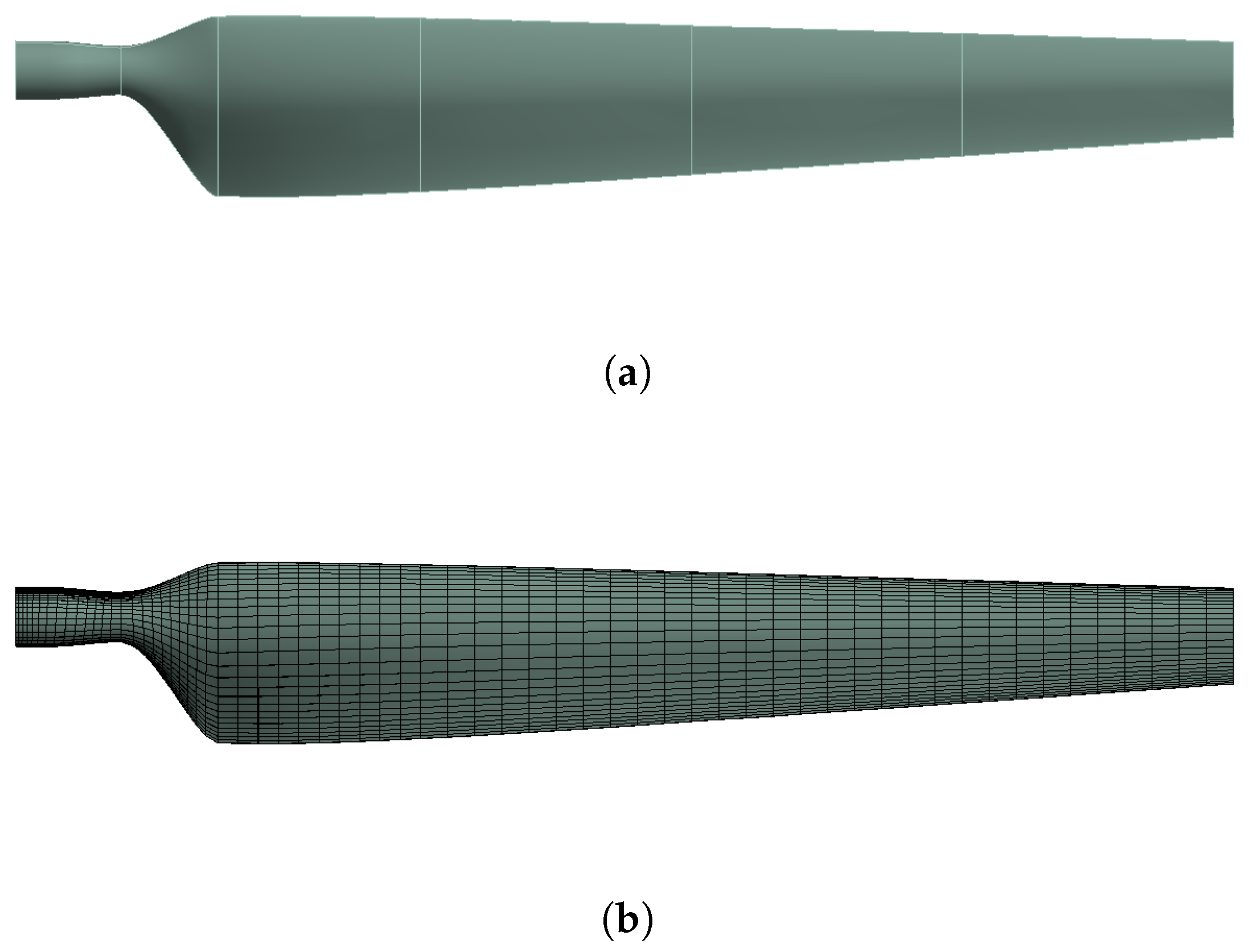
A dynamic tetrahedral mesh with inflation layers is used for the sliding domain around the blade (Figure 2b). The near-wall mesh is built using an inflation zone defined by three parameters: wall-adjacent cell height of 8 × 10 4 m, 15 inflation layers, and a growth ratio of 20%. A wall y + around 30 is obtained, which is acceptable considering that the cell count restrictions, along with the high mesh deformation around the blade boundary, make it difficult to control the aspect ratio within the inflation layer to avoid negative volumes. The rest of the domain is meshed with hexahedral elements (Figure 2a). Given the aforementioned restrictions in computational resources, two meshes are generated: a coarse mesh with 4,929,538 cells and a fine mesh with 8,729,681 cells. The variation total torque acting on the blade shows a relative change of 5.8%, i.e., between 359.5 and 338.7 N m for the considered meshes. The subsequent calculations with the coarse mesh are then justified by this small change to handle the computational expense as best as possible.
The solution of the pV coupling is performed using the explicit SIMPLEC scheme, which, unlike the standard SIMPLE scheme, allows the fine-tuning of under-relaxation factors to control the convergence rate and stability of the numerical solution. Spatial discretization is treated with a second-order scheme, whereas time integration is performed with a first-order scheme to favor the solution stability when large time-step sizes are used.

2.2. Finite-Element Model Configuration for the Structural Problem

The structural response was obtained by considering a transient Finite-Element Method (FEM) solution based on the HHT- α scheme [25], with a time-step size governed by the system coupling process. The geometry of the NREL Phase VI experiment blade is considered (see Figure 3a) and is discretized with linear shell elements. The formulation of the “First-Order Shear-Deformation Theory”, also known as the Mindlin–Reissner shell theory [26,27], is the basis of the SHELL181 element type, which accounts for the transverse shear strain after deformation and, consequently, for relatively thick laminate zones, which in turn are expected in some load-sensitive regions of the blade such as the root.
A fully structured mesh can be created using the topology for each blade surface, as shown in Figure 3b. The orthotropic properties for a single lamina and the laminate layout are defined using the Ansys® ACP Pre module. Since both material and geometric non-linearities are present, a Newton–Raphson iterative procedure under the HHT- α scheme is employed. All parameters that ensure unconditional solution stability are set to the default values.

2.3. Fluid–Structure Interaction Framework

The Fluid–Structure Interaction problem is defined by the coupled solution of three different types of fields. The basic physics models for the flow and blade structure describe the behavior of two fields: flow velocities and pressures on the fluid model and the structure displacement and forces on the solid model. The third field describes the displacement of the flow mesh nodes and is formulated according to a diffusion equation for the node velocity that takes the boundary values from the interface displacement velocity. The three items are described in Table 2.
As expected, the blade surface is completely immersed in the flow field; therefore, the entire entity is assigned as the coupling interface. Since the blade surfaces on both the flow and structure domains are defined from the same source geometry, the association between source and target locations is almost perfect for transferring node displacement and force per unit area. This is reflected in the solution diagnostics from the Ansys® System Coupling, which shows that at least 99% of the flow-side interface nodes are successfully mapped for data transfer.
The System Coupling Module fully governs the coupled solution and considers two data transfers: force per unit area, with the fluid flow solution as the source and the structural solution as the target, and incremental displacement field, with the structural solution as the source and the fluid flow solution as the target. As a strongly coupled problem, the interaction between the flow physics and the structure physics is treated with an implicit scheme described by Chimakurthi et al. [28], implying an iterative data transfer at each coupling step to ensure that both the transfers and the solutions at the end of the time-step are fully converged.
As previously mentioned, the mesh block directly enclosing the blade is defined as a dynamic mesh and is shown in Figure 1. The nodes in this region are displaced according to the motion of the blade structure; this is performed with a smoothing procedure based on a diffusion model which preserves the mesh shape in the proximity of the moving wall and "diffuses" the mesh deformation towards the mesh cells away from the moving wall.
The coupled solution is set to a maximum of three iterations per coupling step. This is performed after revising the solution transcripts and ensuring convergence for each coupling after the third iteration. Finally, a variable time-step strategy is adopted using a sigmoid profile to increase the time-step size from 1 × 10⁻³ s to 5 × 10⁻³ s between t = 0 s and t = 1 s. Unlike a linear profile, which is used for initial simulations, the sigmoidal shape maintains a very small time-step size right after t = 0 s and ensures a gradual and continuous change in time-step size with full control of the duration period for the transition. This is carried out to gain an advantage from a large time-step size when the solution reaches a stable state while maintaining a sufficiently small time-step at the beginning of the simulation, when initial transients usually destabilize the solution if large time-steps are used.

3. Simulation Campaigns

This section introduces the simulation campaigns proposed to validate the numerical solution to the different physical models and the subsequent simulation cases for the wind turbine blade with bend–twist coupling. Further details are also discussed, including the nomenclature, description, wind speeds, analysis subjects, and physics model for each simulation case.

3.1. Validation Cases

The validation of the numerical simulation framework has been defined according to the different physics involved in the problem of a composite wind turbine blade. The experimental results for the NREL Phase VI experiment are used for comparison of the final simulation cases; however, these results cannot be used for validation purposes because details about the structural composition of the blade are not available from the published literature. Instead, the validation of the structure under bend–twist coupling was separated from the validation of the FSI problem. This task was performed with the simulation of a composite D-spar, whereas the validation of the interaction problem was performed with the case of an industrial fan blade for which the entire setup is known. These cases are described next.

3.1.1. D-Shaped Spar with Bend–Twist Coupling

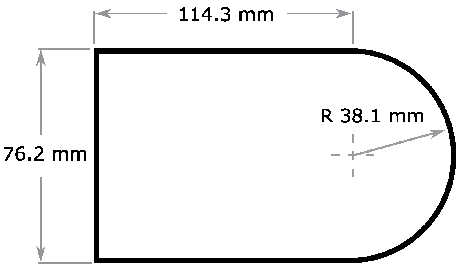
The validation of the structural behavior of the laminated composite subjected to a Type I bend–twist coupling was performed by considering a composite beam with a D-shaped hollow cross-section; this is the validation case “VA01” in Table 3. The simulation configuration is made with the ACP Pre and static structural modules of Ansys, and the case follows the experimental procedure detailed in [6,29], based on a D-shaped cantilever spar conformed with off-axis laminates at 70° and 20° and manufactured with hybrid glass-/carbon-reinforced epoxy. The spar is 1.828 m long, with cross-section dimensions as shown in Figure 4. A transverse vertical load of 1 kN is applied to the beam’s free end.
From the simulations, vertical deflection, equivalent to flapwise deflection, and transverse rotation are retrieved at the section centroid. The locations are defined for five equidistant cross-sectional cuts along the axial direction. Deformation values in the longitudinal direction are obtained at the mid-line of the tension surface.

3.1.2. Air Conditioning Cooler Fan Blade

The validation of the FSI coupling was performed considering the analysis of an Air Conditioning Cooler (ACC) fan blade, as presented by Peters [30] and Peters et al. [31], and supported by published experimental results [32,33]. It considers an aluminum blade with a rectangular platform and symmetric cross-section, similar in shape to a thin diamond with rounded edges. The analysis in [31] addressed the phenomenon of aerodynamic damping, where the blade is subjected to a uniform and constant wind speed with harmonic excitation in the first flapwise mode from the base, with an oscillation of 2 mm in amplitude.
This analysis has been employed in this work to validate the FSI simulation, bearing in mind that the numerical model can be accurately reproduced since the geometric and material properties are fully described; in addition, the boundary conditions derived from the associated experiment can be implemented with the available tools. Given the slender geometry of the blade and the physical contact between assembly elements, this case is expected to be non-linear, being, therefore, more relevant for validation of strongly coupled problems.
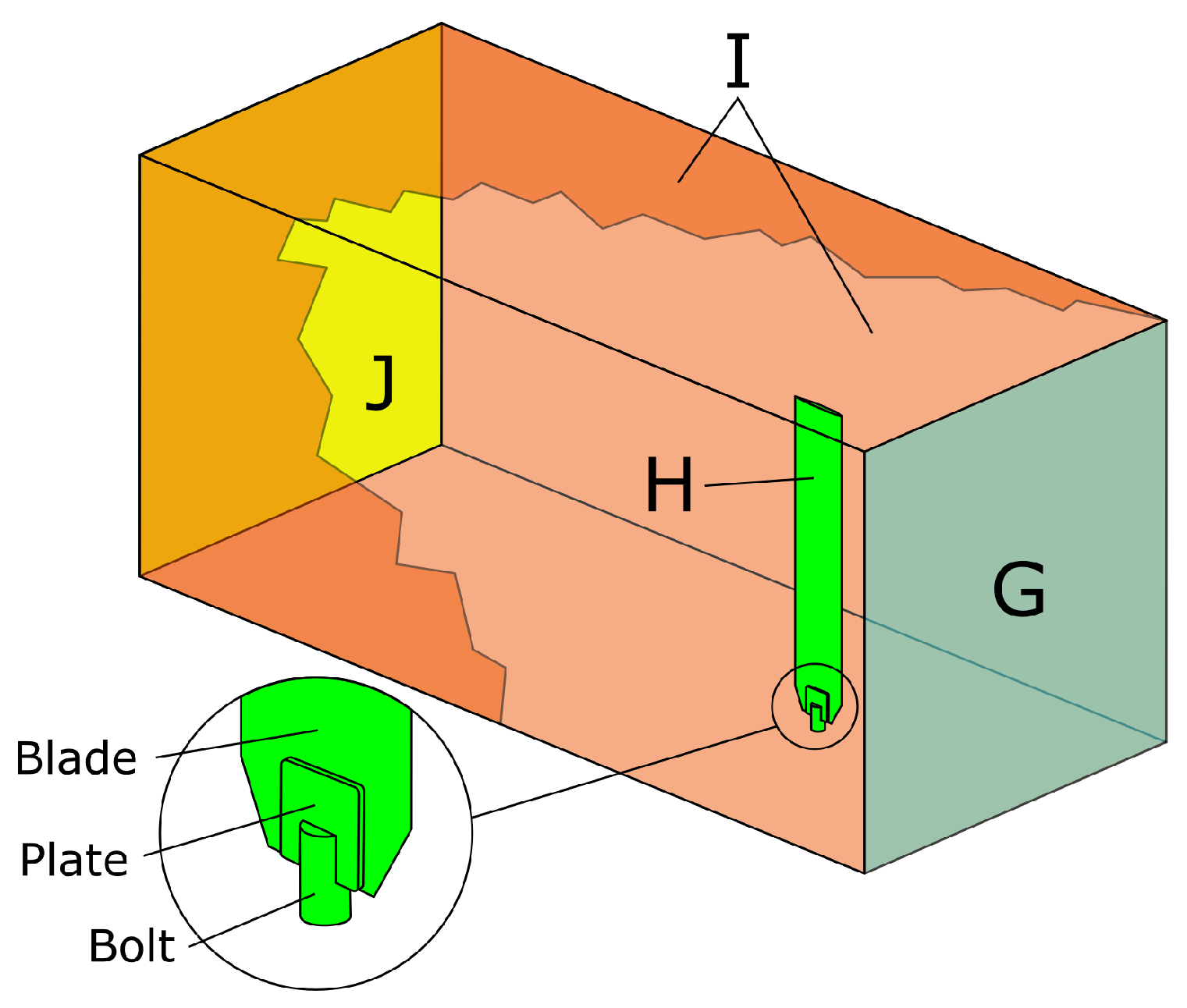
Before the validation of the FSI problem referenced by case “VA03” in Table 3, the fluid solution for the ACC fan blade named case “VA02” was developed. The domain layout shown in Figure 5 considers an inlet wind speed of 20.45 m/s (labeled “G”) and five angles of attack, ranging from 0° to 8° in increments of 2°. The remaining boundary conditions are a pressure outlet labeled as “J” and symmetry regions for the wind tunnel walls, collectively labeled “I” in Figure 5. The no-slip surface for the blade wall is shown with label “H” and a detailed view of the blade root assembly is also included.
Five resulting cases were run for steady, incompressible flow using the SIMPLEC scheme, but the case at 6° was also run for incompressible transient flow with a time-step size of 3.5 × 10 3 s, to reproduce a transient flow solution with moderate separation. The time-step size is defined according to the CFL condition; since the initial simulations consider the PISO solver, this time-step is retained for subsequent simulations with the SIMPLEC scheme. Due to the sharp leading-edge geometry, substantial flow separation can be expected and the k-ω SST turbulent model is used for all simulations. With a cell height of 8 × 10 4 m in the near-wall mesh’s first layer, a y + 30 is obtained.
The settings for the transient simulation are implemented exactly as defined for the flow simulations on the coupled analysis for case “VA03”, with the condition that the time-step size is now governed by the System Coupling module. From the structure side of the interface, a non-linear transient analysis is set up with a prescribed displacement boundary condition at the bolt of the blade (shown in Figure 5), defined by the oscillation profile of the base excitation reported in [33].
During the interaction, the blade surface receives the pressure from the flow solution; at the same time, the surface displacement determines the mesh node displacement to be transferred to the flow mesh in Fluent. The validation is performed first by comparing the aerodynamic coefficients to ensure that the turbulent, and unsteady flow description is close to the experimental and numerical results. Secondly, the validation compares the tip displacement results with those reported in the literature [33].

3.2. Study Cases

The effect of composite laminates with bend–twist coupling behavior is explored from a series of comparative analyses also based on numerical simulation and comparison with the behavior of a reference “neutral” composite structure for the same blade geometry. The series of simulation cases is described next.

3.2.1. Equivalent Blade Structure

This section describes the definition of a laminate sequence with comparable structural properties, in terms of flapwise bending stiffness, axial stiffness, and mass distribution, to the properties of the experimental blade reported in [23]; this case is called “VA04” in Table 3, which includes the nomenclature for all of the simulations considered in this work. Since a composite wind turbine blade can be designed in an infinite number of material and laminate layup combinations, the present work does not aim to match exactly the properties of the experimental subject; instead, an approximate structure is pursued as a means to establish a sound reference for assessing the effect of coupled laminate materials.
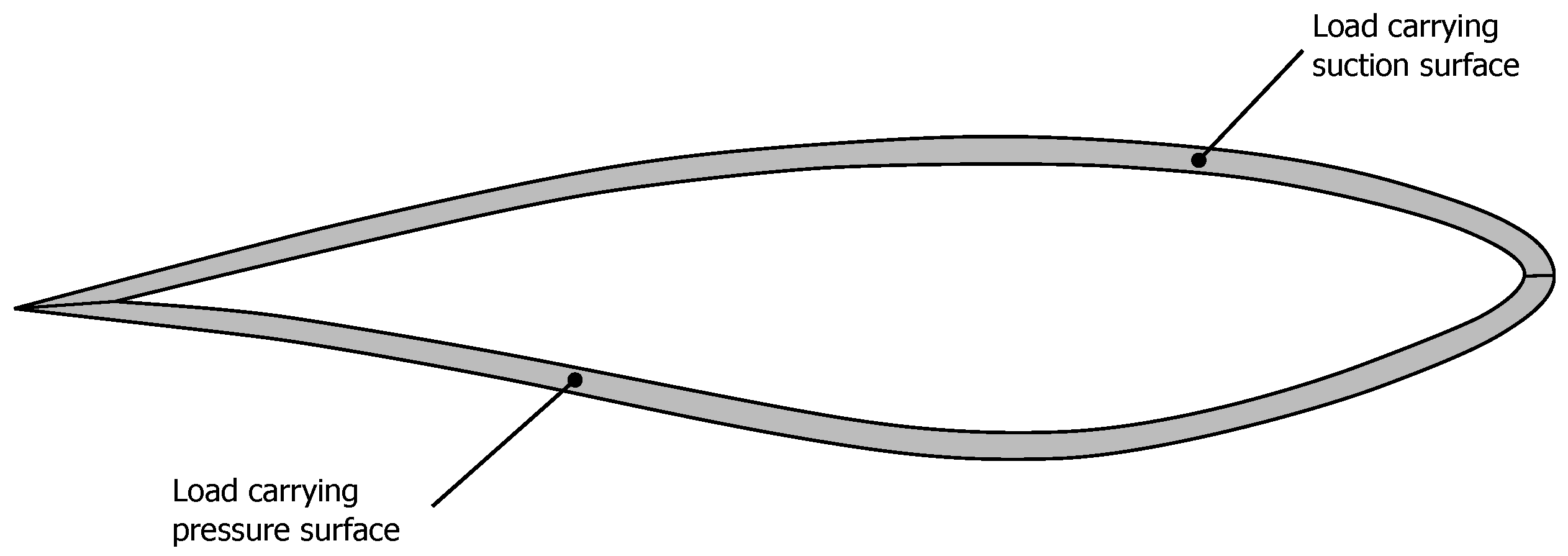
A similar task was carried out by Chujutalli et al. [34] and Lee et al. [35]. These works proposed a set of laminate mechanical properties and stacking sequences to obtain a 3-D equivalent numerical model of the NREL Phase VI blade. It must be said that the present work considers only the shells of the blade as the load-carrying members, resulting in the simpler structure shown in Figure 6. This is justified by the interest in small wind turbines, for which simplified blade structures are often advantageous.
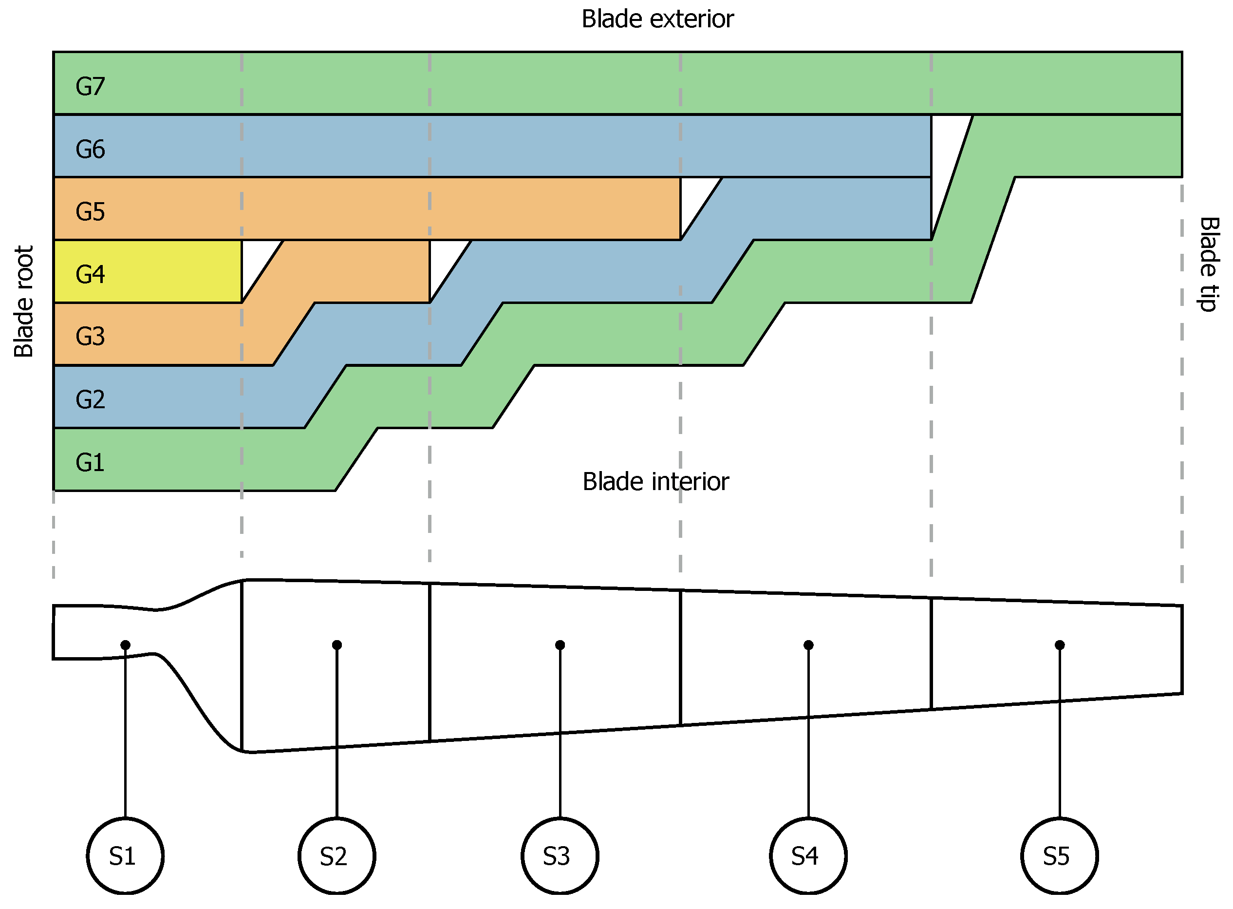
A set of nine material properties was adopted from [34] for modeling the blade structure with shell elements under the assumption of negligible out-of-plane deformations, supported by the consideration of very small transverse dimensions relative to the blade length and width and, also, by the consideration of in-plane loads only. To resemble the reduction in skin thickness towards the blade tip, five segments along the blade span are defined, in which a series of laminate drop-offs are placed according to the desired thickness and mass distributions (see Figure 7). The upper limits for each one of the blade segments (S1, S2, S3, S4, and S5) are 1.257 m, 2.012 m, 3.018 m, 4.023 m, and 5.029 m, measured from the center of rotation.
The proportion of plies in each segment relative to the orientation is similar to that in Chujutalli et al. [34], but the number of plies and the orientation varies. For this work, the entire structure is constituted of a carbon/epoxy composite, orientations other than 0° are considered, and a higher number of plies per section is proposed. The laminates are separated into seven groups (G1 to G7), each with a different number of plies and stacking sequence as shown in Table 4. One of the critical aspects when defining the laminate sequences for each ply stacking group is to avoid macro-mechanical coupling, which is verified by inspecting that the bend–twist coupling terms in the laminate stiffness matrices are zero.
The stacking sequence of the laminate groups as described by Table 4 is depicted in Figure 7. The drop-offs between adjacent laminate groups are specified using the five-blade segments shown in Figure 7; this way, the expected mass distribution is obtained. An important characteristic of this layout is that the drop-offs between individual plies are not considered; therefore, all the plies in a specific group have the same lengthwise extent.
In order to obtain the required nose-down rotation from a blade with bend–twist coupling, the general arrangement of the off-axis fibers must be as shown in Figure 8, and the laminates of the suction side must mirror those of the pressure side. This requires that, for a coordinate system consistently oriented outwards for all blade surfaces, the off-axis fiber orientation of the suction side is opposite to that of the pressure side.
The second stacking sequence corresponds to the case “VA05” and is described in Table 5. This is a modified version of the laminate used in the sensitivity analysis “VA06” of the tip rotation with respect to the off-axis fiber angles, denoted in Figure 8 by θ . The results reveal that, for an angle of 20°, the tip rotation angle reaches its maximum value. From the stacking sequence from case “VA06”, three important changes are deemed to define the final blade with bend–twist coupling represented by the case “VA05”: the ply orientation for bend–twist coupling is extended to the laminates in group G4, the plies at 0° in groups G2, G3, G5, and G6 are changed to off-axis plies, and two plies at 0° are removed from laminate groups G1 and G7.
The first of these changes aims to increase the overall blade rotation by enabling the coupling effect to take place throughout the entire laminate thickness, whereas both the second and third changes are performed to increase the proportion of off-axis plies in the whole laminate, considering the findings of Hayat and Ha [17], which suggest that off-axis ply proportion has a dominant effect on the coupling rather than the total amount of off-axis plies.

3.2.2. Computation of Blade Loads

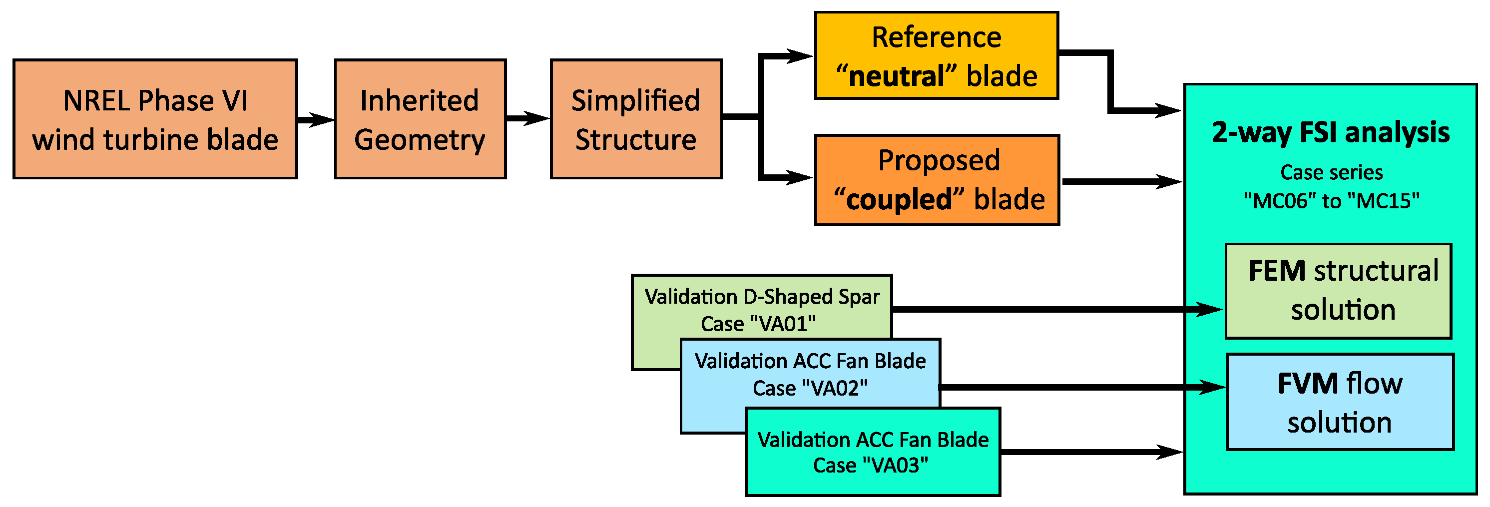
The FSI simulations for blade load prediction were performed for five wind speeds, namely, four cases at 7, 10, 13, and 20 m/s, to obtain the rotor steady torque curve, and one case at 39.5 m/s for the assessment of loads at extreme wind conditions. These simulations correspond to “MC06” to “MC15” in Table 3. For each wind speed, two simulations take place, one for the neutral blade of case “VA04” and one for the coupled blade of case“VA05”. A representation of the workflow including the validation and main simulation cases along with the definition of the subjects of analysis is shown in Figure 9.
The results from the simulation cases involve rotor loads and torque and include additional data from auxiliary simulations. Although the details are omitted, the additional results from case “AX16” are produced with a one-way FSI analysis based on the Blade Element Momentum theory for the aerodynamic load calculation. These results are used to complement the analysis of the structural coupling on the annual energy production. The results of cases “AX17” to “AX20” are used to complement the CFD analysis of the rotor loads in steady wind conditions.

4. Results

4.1. Validation Cases

4.1.1. D-Shaped Spar with Bend–Twist Coupling

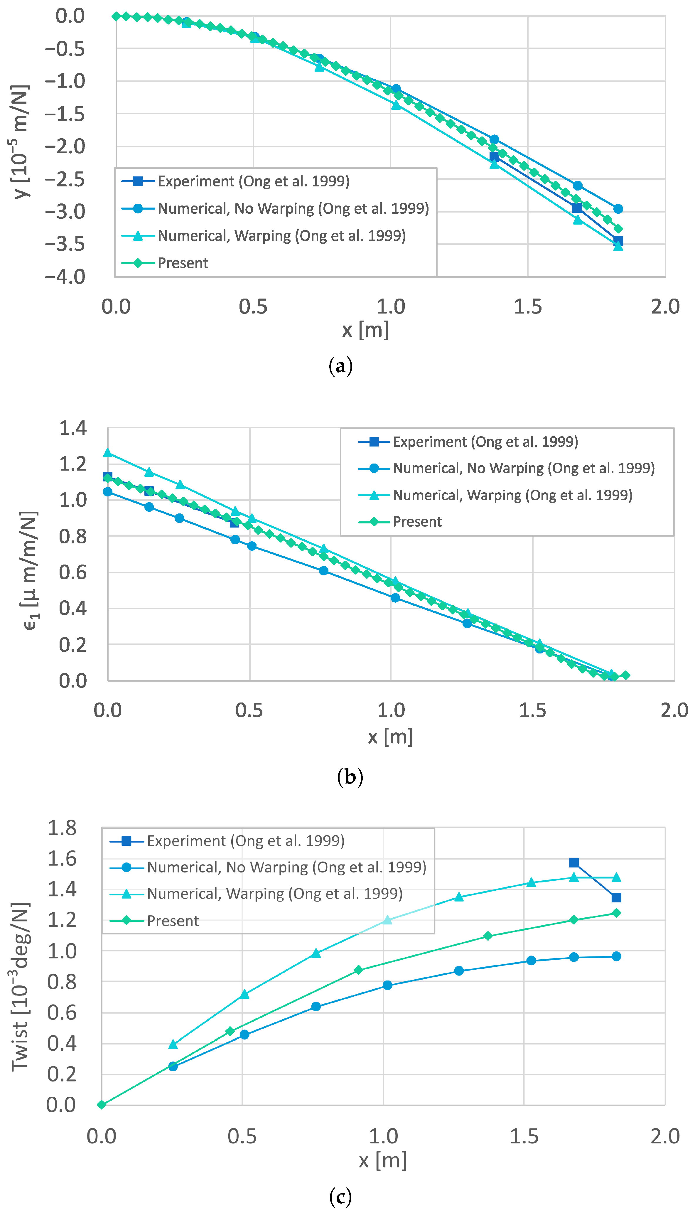
The numerical results considered for the steady loading case are the transverse deflection and torsional deformation sampled at the centroids of different sections, as well as the strain along the tension surface of the beam. These results are compared with experimental measurements and numerical estimations from Ong and Tsai [29]. The vertical deflections are shown in Figure 10a, where it can be noticed that the general behavior along the longitudinal axis of the present results is consistent with previous numerical and experimental results. The L-2 norm of the relative error is calculated for all numerical results with respect to the experimental values from [29]. Vertical deflections result in a 5.6% relative error norm, reflecting a satisfactory solution from the finite-element shell model used here.
In a similar fashion, the longitudinal strain ( ϵ 1 ) shown in Figure 10b reflects an acceptable prediction when compared to the reference experimental data, with an L-2 error norm of 0.76%. The comparison for the torsional deformation in Figure 10c shows that the predictions of bend–twist coupling with the present SHELL181 FEM model approach the experimental values for the tip loads.
Two main findings arise from the plots in Figure 10c: first, the present results are bounded by the 1-D numerical predictions reported by the reference numerical works [6,29], and, second, the present results confirm the monotonic increase in the twist angle along the longitudinal direction, contrary to the results from experiments. Regarding the experimental results in [6,29], it must be said that twist angles do not correspond to several measurements with a constant load but rather to linear regression for multiple measurements with different load magnitudes. The measurement error might cause the unexpected behavior that the authors reported, as they measured rotation at two locations only and took the respective averages from the multiple random measurements. This leads to an important relative error of 18.8%.

4.1.2. Air Conditioning Cooler Fan Blade

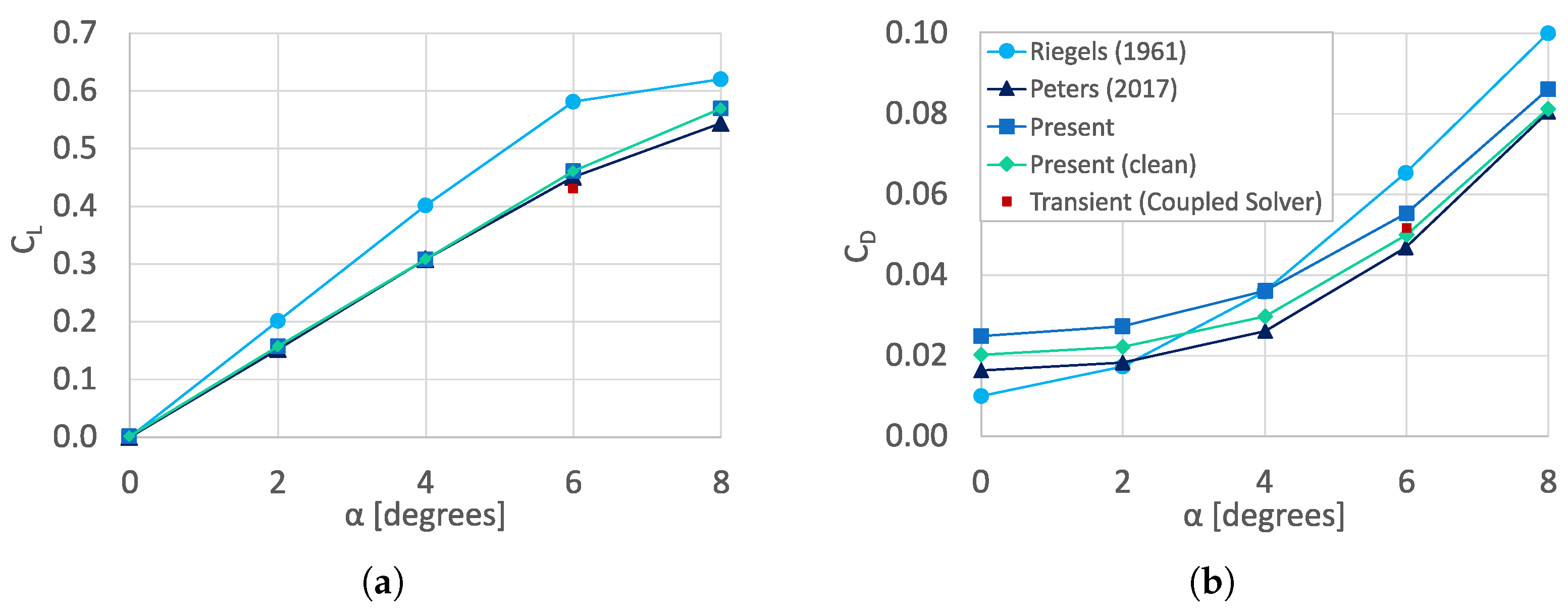
For the case “VA02”, steady-state predictions for steady-state C L are shown in Figure 11a and resemble those of Peters et al. [31]. In this figure, the label “Present” represents the full blade geometry, whereas “Present (clean)” stands for the blade without the bolt at the base, labeled as the reference results provided by Peters [30] and the reference results for a flat plate from Riegels [32].
The geometries with and without the base bolt are considered simultaneously to explain the result discrepancies that are presented later. The results for a transient solution at 6° are also included with the label “Transient”. The numerical predictions are satisfactory for all angles of attack, with larger but still acceptable differences for α = 6 ° and α = 8 ° . The experimental solution, presented by Peters et al. [31] and Riegels [32], keeps, for most of the cases, a noticeable difference concerning the numerical results and also concerning the reference numerical results from [31]; as explained by Peters et al. [31], the discrepancy might be because the experimental study is performed on a 2-D wind tunnel set up, whereas the numerical cases reproduce a 3-D scenario where the blade tip is freely exposed to the incoming flow.
The transient solution for α = 6 ° slightly underpredicts steady-state lift results; however, the transient computation remains acceptable, considering that the flow conditions at this angle of attack might involve a degree of separated flow near the trailing edge, a permanent challenge in terms of accuracy for the implemented turbulence model.
In contrast to the results obtained for steady-state C L (see Figure 11a), important differences between simulations for the blade with and without the bolt can be noticed in Figure 11b for the drag coefficient, C D . In general, the simulation with the full geometry (“Present”) shows a larger overprediction of C D regarding the reference case of Peters et al. [30,31].
The root assembly of the fan blade is not expected to contribute to lift, being constituted by an axisymmetric cylinder and two flat plates, confirming the initial premise: the computed lift from Figure 11a is not affected by this change while the computed drag becomes closer to the reference for both steady and transient cases. The evident difference between experimental and numerical C D for α 2 ° might signal that the presence of drag due to lift in the 3-D case is responsible for the underestimation compared to the experimental C D .
The validation of the FSI problem, identified as “VA03” in Table 3, has been performed considering the experimental results published by Basson [33]. The validation work presented here adopts three reference cases, where the blade is fixed at a 9° angle while the inlet wind speed is set to 20.05 m/s, 15.03 m/s, and 10.72 m/s. The experimental work of Basson [33] consists of 50 instantaneous measurements of the blade tip displacement with the base excitation mechanism, as described in Section 3.1.2; since these measurements are random, the comparison with the experimental results uses an average of the displacement history for each simulation case.
The time history of the numerical blade tip displacement is shown in Figure 12 excluding the initial transients for each data set. Additionally, the average numerical displacement is presented and compared to the average of the experimental data reported by Basson [33].
The first case, corresponding to the simulation with an inlet wind speed of 20.05 m/s, is presented in Figure 12a, showing that the average numerical tip displacement closely matches the experimental data, obtaining a relative error of 5.6% with respect to the experimental value. As observed in Figure 12b,c, the average numerical tip displacement is relatively close to the average experimental value for the other two speeds considered here, with relative error measurements of 11.2% at 15.03 m/s and 13.2% at 10.72 m/s.
The small error estimates reveal an acceptable accuracy; however, it is worth noticing an increase in the relative error when the inlet wind speed is reduced from 20.05 m/s to 10.72 m/s. At least two reasons can be pointed out for this behavior. Firstly, the change in wind speed from 10.72 m/s to 20.05 m/s implies a change in the Reynolds number by one order of magnitude; considering air at standard conditions and a blade chord of 0.12 m, this may induce a change in the separation behavior.
The second reason is related to the flow separation phenomena because the angle of attack at a given section of the fan blade results from the combination of two components of velocity: the inlet flow velocity and the relative vertical velocity caused by the oscillation. The geometric relationship between the inlet and transverse velocities dictates that the angle of attack for a given blade section should be larger when the inlet wind speed is lower. The current assumptions on the turbulence modeling added to the thin plate and sharp leading edge geometry of the fan blade can result in poor predictions for separated flows, which in this case alternates between both sides as the blade vibrates due to the base excitation.

4.2. Study Cases

4.2.1. Equivalent Blade Structure

The verification of the structural properties for the case “VA04” shown in Table 3 was performed using the software NuMAD [36]. With the blade property extraction functionality, the resulting mass, flapwise, and axial stiffness distributions are extracted and compared to the properties of the experimental blade. Further information on this methodology can be found in [37]. The mass distribution of the present blade corresponds purely to the mass of the composite materials for each blade surface; this is worth mentioning because the experimental model has additional elements that contribute to the total mass but not to the global structural behavior of the blade.
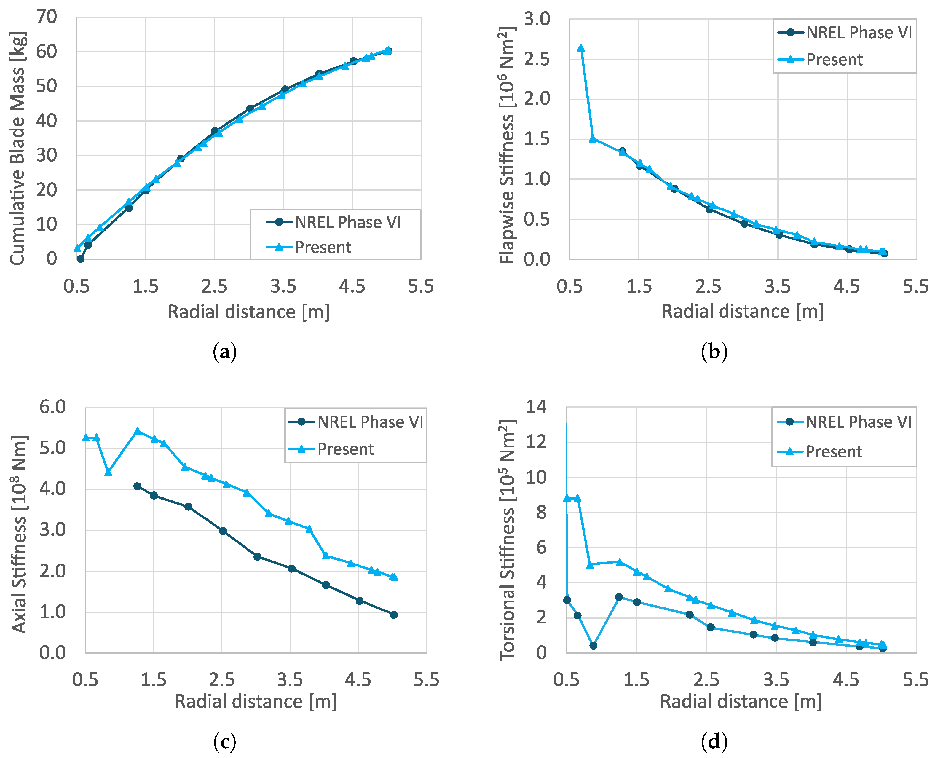
A resulting distribution for cumulative mass, shown in Figure 13a, reveals good agreement between the proposed blade model and the experimental one. The total mass for the resulting blade model is close to 60 kg, keeping its similarity with the 60.3 kg reported from the experiment [23]. The methodology for extracting stiffness properties from the numerical model of the blade is omitted here, but the reader is referred to [37] for further details. The distribution of flapwise stiffness plotted in Figure 13b shows a similar match between the proposed and experimental blade models for most of the blade, except the near root sections, where the present laminate is thicker than the experimental one. The flapwise stiffness for mid- and outer-blade sections is close to the experimental blade stiffness at the flapwise deformations that should eventually exert a coupled twist occur at those blade regions.
The resulting distribution for axial stiffness in Figure 13c shows that the proposed numerical model noticeably overestimates this property along the entire blade span. This situation does not compromise the validity of the proposed model for comparison with a bend–twist coupled counterpart, for the reason explained above, i.e., the torsional deformation response of the bend–twist coupled blade is mainly determined by the bending deformation in the flapwise direction rather than by the axial deformation. The differences in the axial stiffness with the experiments are noticeable and this may be caused by the larger extension of the load-carrying members in the present blades.
The blade structures of cases “VA04” and “VA05” differ from the load-carrying D-spar of the experimental subject because the latter extends only 40% of the chord length, whereas the present blades have a pair of load-carrying aerodynamic surfaces, comprising the entire blade section. In other words, there is more stiff material in a greater extent of the cross-section and, therefore, a higher axial stiffness is obtained. Similarly, the additional material added towards the trailing edge of the blade results in a considerable amount of fibers being placed away from the elastic axis and, consequently, induces a greater torsional stiffness, as shown in Figure 13d.
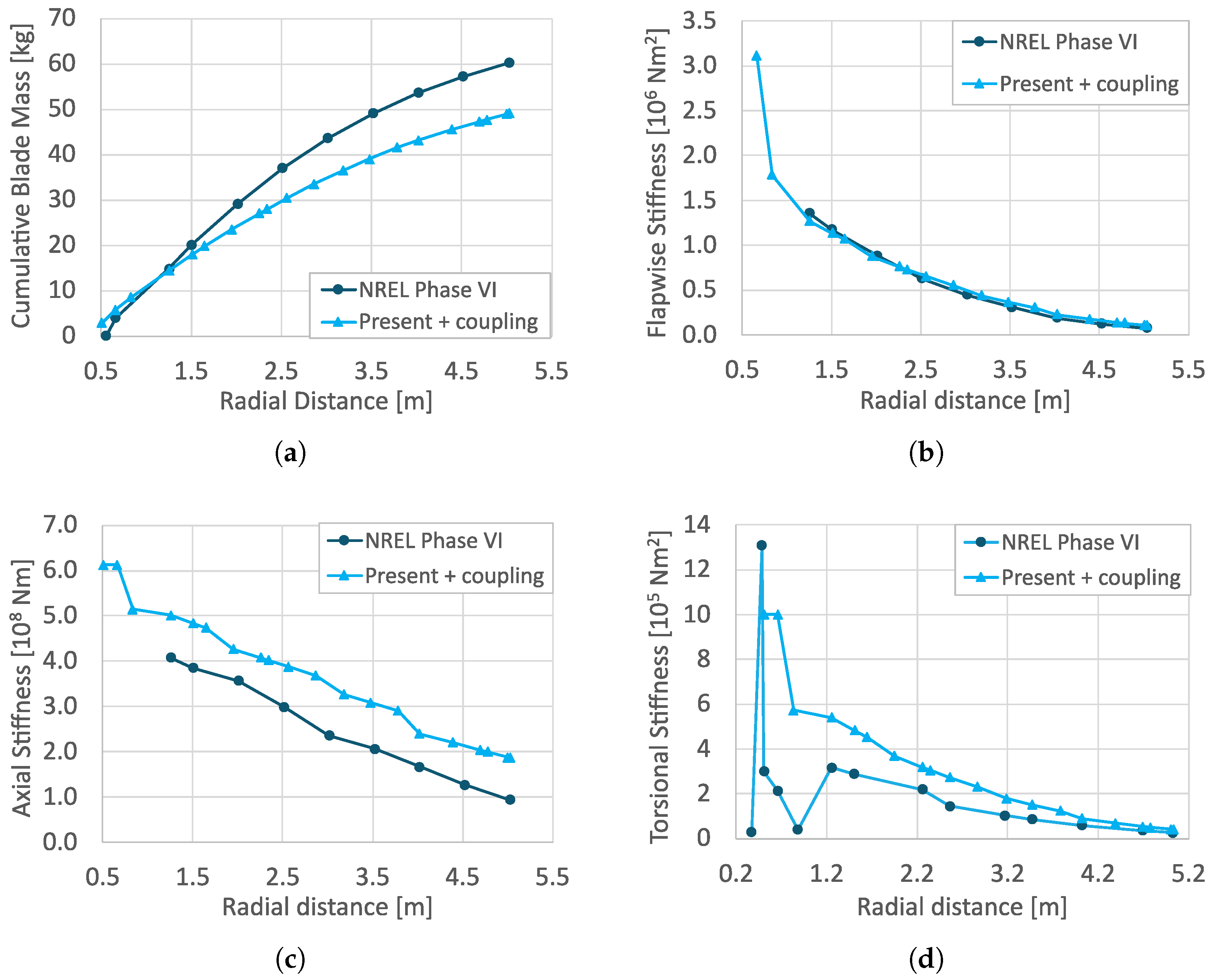
Most of the relevant properties obtained in case “VA05” of Table 3 remain close to the properties of the NREL Phase VI experimental blade or the properties of the baseline structural design for case “VA04”. According to the cumulative mass distribution presented in Figure 14a, the present blade is lighter by approximately 11.6 kg than the reference blade, mainly due to the reduction in 0° plies.
The flapwise bending stiffness (Figure 14b) is significantly closer to the reference stiffness when compared to the other stiffness properties (Figure 14c,d), and this is precisely one of the key points from the present task, considering that the coupled blade rotation occurs from a bending displacement in the flapwise direction. In fact, the reduction in 0° plies across the entire length of the blade contributes to a reduction in axial stiffness, at least for the tension side of the blade; in consequence, the stiffness distribution for the coupled blade in Figure 14b is closer to the reference than the neutral reference blade in Figure 13b.
Additionally, the flapwise stiffness distribution for the root of the blade is visibly higher than for the rest of the blade, due to the accumulation of fibers that reinforce the core of the laminates at this structurally sensitive area.. The results for axial and torsional stiffness in Figure 14c,d reveal a stiffer blade than the experimental one but still close to the mechanical properties in the baseline design shown in Figure 13.

4.2.2. Assessment of Blade Loads in Normal Operating Conditions

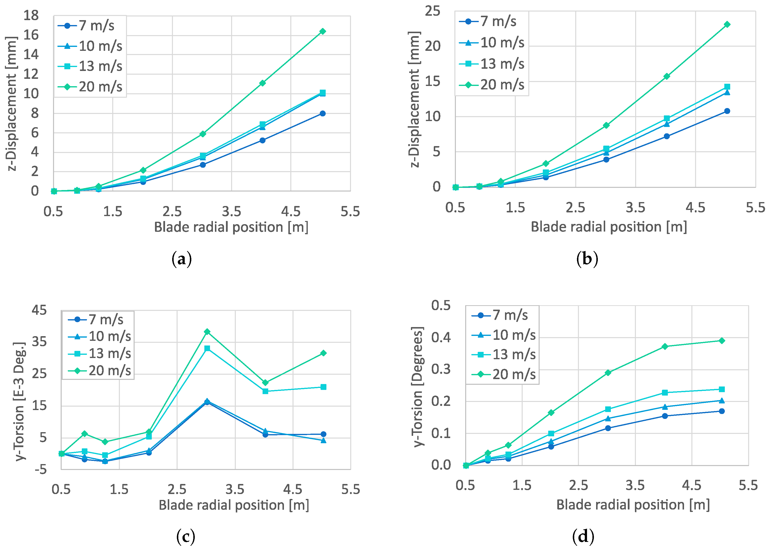
This section presents the results corresponding to the neutral blade operation under steady wind of cases “MC06” to “MC09” and to the coupled blade operation under steady wind of cases“MC11” to “MC14”, according to Table 3. Seven locations are used for sampling the vertical displacement along the z-axis and the torsional rotation in the longitudinal or y-axis. Figure 15a,b shows flapwise displacement in the negative z direction.
At first glance, the results reveal the typical deformation profile for a cantilever beam and also indicate that the displacement magnitude increases in direct proportion to wind speed. The latter finding is expected for a constant angular speed turbine. There is also a hint of non-linearity concerning wind speed when the displacements for outboard blade stations are inspected; for instance, the results at 10 m/s and 13 m/s seem to be mutually clustered and more separated from the results at 7 m/s or 20 m/s. This has already been reproduced in similar analyses, for instance, in the work of Lee et al. [38]. Aerodynamic instabilities associated with flow separation are likely causes for the non-linear behavior in rotor loads.
Furthermore, the flow conditions responsible for stall are between 10 m/s and 13 m/s, as, in this range, the torque curves reach their peak values before decreasing at higher wind speeds; in consequence, the non-linear aerodynamic loads around peak torque are the probable cause of non-linear deflections at these wind speeds.
When comparing the magnitude for maximum displacement, which occurs at the blade tip ( r = 5.029 m) at 20 m/s, the coupled blade results show a larger magnitude by approximately 6.6 mm (see Figure 15a,b). Despite aiming for flapwise bending stiffness as close as possible to the one from the NREL Phase VI blade, the reference blade model is slightly stiffer between the inner and intermediate blade sections than the coupled one, as can be observed when comparing Figure 13b and Figure 14b.
The torsional displacement for the reference blade model, shown in Figure 15c, reveals a relatively weak coupling between flapwise bending and torsional displacements since the magnitude of blade section rotations is of the order of 1 × 10 2 degrees; furthermore, no proportionality relation can be discerned between rotations and deflections. The rotation angle has a non-monotonic variation while it appears to increase. The maximum rotation is observed at the fifth probe location counted from the blade root ( r = 3.013 m); this happens for all wind speeds. It is likely, that aerodynamic forces are being applied at a distance from the elastic axis of the blade, resulting in the observed rotation for the reference blade.
When defining the laminate groups for the reference blade, an analysis with classical lamination theory shows that the bend–twist coupling terms in the force and moment resultants for rectangular plates are zero. Even though the laminates in the neutral blade have no bend–twist coupling, the blade geometry is more complicated than a rectangular flat plate and the laminate drop-offs differ from the controlled calculation on the flat panel; therefore, neither material-based coupling nor geometry-based coupling should be ruled out of the reference blade model. Assuming thin plate theory, an order 1 × 10 2 change in angle of attack should result in an order 1 × 10 3 change in lift coefficient; therefore, aerodynamic forces should be coupling-insensitive in the reference model.
When observing the results for the blade structure with bend–twist coupling in Figure 15d, an evident contrast arises to the neutral blade. First, the bend–twist coupling increases the order of magnitude in blade rotation to 1 × 10 1 , which is valid at all wind speeds in the middle and outer blade sections. At r = 1.257 m, where the third sampling point is located, the rotational displacement profile shows a steep change in slope, most likely due to the marked change in thickness as the core plies near the root meet the transition area between the cylindrical and airfoil shapes (Figure 7).
The prediction of torque values from the robust FSI analysis of the reference and coupled blades is presented in Figure 16a under the labels “Reference” and “Coupled”, respectively, along with the experimental values and a steady-state reference with the label “Steady CFD”, which considers a fully rigid blade. The shape of the torque curves for the reference and coupled blade are relatively close to each other at all wind speeds, with the torque of the latter being slightly higher than the torque of the former.
This indicates that the pitch towards the feather via bend–twist coupling has a positive effect in increasing the amount of torque delivered by the rotor, with the increase being stronger at 13 m/s; in contrast, the reference and coupled power curves show little difference at 25 m/s, an unexpected result given that the coupling is stronger at high wind speeds. This may be attributed to the observed fluctuations for these two data series, considering that they are unsteady simulation results that could be averaged through a larger time interval to better reflect the long-term stabilized result. From the data of the neutral and coupled series in Figure 16a, it is also evident that the numerical calculations with the robust simulation framework result in torque underpredictions regarding the experimental data published in the measurement campaign from the NREL Phase VI experiment [39,40,41,42].
The discrepancy between numerical and experimental results is more notorious at 10 m/s and 13 m/s, where the prevailing separation and stall effects strongly define the aerodynamics around the blade. This is a critical issue in the prediction of rotor loads for fixed-pitch wind turbines which is not taken into account in the mathematical model of Ansys® Fluent.
Flow separation and its role in stall behavior cannot be predicted with the k–ω SST turbulence model, which represents a relevant limitation in the present co-simulation framework. The high angles of attack at which the relative flow intercepts the blades, for wind speeds above 10 m/s, are challenging scenarios for the numerical model used in the transient analysis for the “Coupled” and “Reference” series. Additionally, the results from the “Steady-CFD series” that are produced with a much finer mesh show that the aerodynamic loads are highly dependent on the resolution of the near-wall mesh and the resulting turbulence modeling for this region.
The prediction of the flapwise and edgewise blade root bending moments is important to assess the blade’s structural performance. Particularly, the flapwise bending moment is perhaps the most critical for the structural integrity of the blade root assembly; it is dominated by the bending action of the thrust force which has contributions from both drag and lift forces. The prediction of flapwise bending moment from the robust simulation framework is shown in Figure 16b, revealing three main outcomes: the results are close to the experimental measurements, the flapwise bending moment increases almost linearly with the wind speed, and the action of bend–twist coupling is stronger at the higher wind speeds.
On the other hand, Figure 16c shows the edgewise bending moments with a slight underestimation for all wind speeds except at 20 m/s; in addition, the standard deviation of the experimental edgewise bending moment is relatively large, at least compared to other measured quantities, such as the shaft torque.
A second part of the comparative analysis under the case name “AX16” (Table 3) is performed using the BEM model with dynamic induction, stall delay, and dynamic stall effects. The aerodynamic solution provided by the BEM model is now interacting with a very simple approach consisting of an interpolation of the blade local torsion as a function of the radial position and free-stream wind speed, using, as inputs, the results from simpler, 1-way FSI co-simulations.
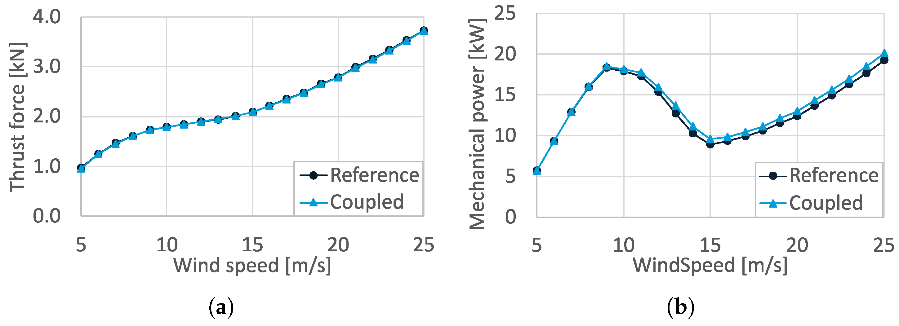
Two sets of results are initially generated to compare the reference blade and the coupled blade, namely, curves of thrust versus wind speed, and curves of power versus wind speed. Since the NREL Phase VI wind turbine is a constant speed machine, the mechanical power is computed as the product between torque and the 72 RPM angular speed; this results in the characteristic power dip at wind speeds above rated, which implies that the wind turbine operates at sub-optimal power coefficient in such a wind speed range.
According to Figure 17a, the bend–twist coupling, as implemented here, seems to have a small effect on the rotor integral thrust force. The reduction in thrust force, which is a desirable scenario from a load mitigation point of view, is barely noticeable. Similarly, the coupling does not seem to increase loads in the axial direction; therefore, the design of other components such as the tower and foundations is not impacted negatively by the use of a blade with bend–twist coupling.
By observing the power curve predictions from Figure 17b, one can immediately appreciate a different scenario, as the power for the bend–twist coupling blade is consistently higher than the reference power for a broader range of the operating envelope. For wind speeds beyond 10 m/s, the bend twist coupling is effective in increasing rotor torque by inducing a local torsion into the feather position. When pitching the blade into a feather, the angle of attack tends to decrease and, even though lift can be decreased as well, the reduction in drag forces might be significant enough to result in an overall torque gain.
A more meaningful picture can be observed by judging the increment in the energy output for a particular period. This is performed by computing the AEP for both power curves and assuming a Rayleigh distribution for the wind resource. The modest torque increments due to bend–twist coupling described earlier are reflected in substantial increments in the AEP ranging between 1.5% and 3% for average wind speeds between 7 m/s and 11 m/s. This result must be taken with caution since the Rayleigh distribution has a considerable dispersion of occurrences for wind speeds in the higher end of the envelope, where the effect of bend–twist coupling is noticeable.
A more conservative picture is obtained from the context of the present research, by considering a Weibull probability distribution for the coastal locations of Barranquilla and Santa Marta in northern Colombia. Assuming a set of scale parameters of 11.5 and 11 m/s and shape parameters of 3.75 and 3.5 [43], the AEP increases by 2.7% and 2.4%. This information corresponds to wind resource estimations at a height of 10 m. Considering the reference hub height of 17 m for the NREL Phase VI experiment, it is reasonable to assume an optimistic outcome because the reported wind speeds with the highest probability exceed 11 m/s for the reported locations.
This means that the use of laminate composites to induce a pitching deformation towards the feather using the induced bend–twist coupling is an effective means for improving the energy output of a small, fixed-pitch wind turbine. Because a constant angular speed is considered, the power output is bound to decrease at wind speeds above the rated value, hence creating an interesting scenario for increasing power. In contrast, the question of how bend–twist coupling would perform as a power regulation mechanism for the considered rotor remains open since angular speed is not modified and the blade twist is rather modest in comparison with typical pitch magnitudes in modern control systems.

4.2.3. Assessment of Blade Loads in Extreme Wind Conditions

The last simulation cases performed, as full two-way interaction problems, are labeled “MC10” and “MC15” following the nomenclature in Table 3. The rotor is now assumed to be in parked conditions with a wind speed of 39.4 m/s, equivalent to the extreme wind model (EWM) for a Class III small wind turbine, as stipulated in [44]. Flapwise displacement and torsion results are shown in Figure 18. Torsional displacement is characterized by a relatively small order of magnitude ( 1 × 10 2 ) and a non-monotonic increase along the radius in the case of the reference blade shown in Figure 18a.
The fact that the reference blade has a very small coupling between bending and torsional displacements results in a fluctuating profile, explained by two possible situations: (a) the magnitude of the time-dependent fluctuations may be comparable to or higher than the torsional deformation due to the natural coupling caused by the aerodynamic moment, or (b) a differential aerodynamic moment causing larger rotation magnitudes at inner and medium-outer sections due to the continuous change in blade chord length and torsional stiffness. The torsional displacement of the blade with bend–twist coupling, seen now in Figure 18b, has a defined tendency to increase with the radial position and reaches a maximum of about 0.64° at the tip of the blade.
The nature of this case from an aerodynamic perspective is, in essence, the same as a flat plate normal to the flow, since the blade is not rotating and much of its length is placed at an almost 90° orientation relative to the free-stream wind; for this reason, drag force instead of lift can be expected to be the dominant load driving the deformation of the blade.
It is also sound to expect that the aerodynamic moment acting on the blade along its longitudinal axis is partially responsible for the torsional displacement adding to the coupling-induced rotation; this is a very likely scenario, as drag force exerts a normal pressure on the blade in the same direction as the flapwise deflection.
The magnitudes of the three bending moments and the magnitudes of tangential and axial force acting on the static blade are organized in Table 6 to highlight the relative change for the coupled blade concerning the reference structure. As a result of the coupling, the flapwise bending moment is increased by 0.3% concerning the neutral blade. The axial force, generated mainly by drag due to the blade’s static position, sees an equally small increase of about 0.2% concerning the corresponding value for the neutral blade. However, it is very important to bear in mind that the magnitudes of these reported differences must be supported by further analysis on the uncertainties for the FSI simulations.
The results from Figure 17a also show a small change but are subject to uncertainties despite being estimated with a different model. An observed 3.9% increase in the edgewise moment is consistent with the 3% increase in tangential force, and both outcomes are a consequence of the observed torsional displacement from Figure 18b, which decreases the angle of attack through a pitch action towards feather, especially for the blade tip region.
By reducing the angle of attack along the blade length, some degree of lift force may contribute to the aerodynamic force resultant, since not only the inboard region of the blade but also other sections near the tip are likely to be in a deep stall flow condition, as opposed to the normal flow scenario; in consequence, an increase of about 16 N in tangential force is experienced.

5. Conclusions

According to the results, the blade structure with bend–twist coupling successfully undergoes a torsional deflection along its longitudinal axis in response to an aerodynamic load. This is observed at the same time that the flexural and torsional stiffnesses of the reference and coupled blades are maintained as close as possible to the properties of the experimental blade. The main analysis of the coupled blade structure, other than the two-way FSI studies in the robust simulation framework, is condensed into a series of steady-state, one-way interaction simulations that demonstrate the efficacy of the coupled composite structure.
The reference blade exhibits small torsional displacements mainly due to time-dependent fluctuations and changes in the blade chord length along the radius. The results for the one-way analysis reflect that the use of bend–twist coupling as a mechanism for passive blade torsion effectively induces a positive change in the resulting annual energy production, with a 3% increase considering a Rayleigh distribution with an average wind speed of 11 m/s. This is shown for a reference wind resource based on the Rayleigh distribution and for two actual wind resources at coastal locations, characterized by the Weibull distribution.
The torsion mechanism is defined by a torsion towards the feather position, which decreases the angle of attack and, in consequence, results in an increased lift-to-drag, which implies that the reduction in drag outweighs the reduction in lift. Because lift is reduced, a secondary consequence of the proposed actuation mechanism is a reduction in the total thrust force over the rotor blades for most of the wind speeds within the operation range, particularly between 15 and 25 m/s, at which the total thrust force sees a reduction of about 0.35%.
Even though a more substantial reduction in thrust force would be a highly desirable scenario, the modest change observed here is still favorable because it suggests that the improvement in rotor torque and, hence, power comes at no cost from the point of view of the thrust loading, which eventually impacts the cost of the entire turbine assembly.
The feasibility of a blade with bend–twist coupling is demonstrated from a structural point of view from the analysis of blade root loads under extreme wind conditions with a 39.4 m/s wind speed in parked conditions. As a consequence of the bend–twist coupling, the flapwise bending moment increases by 0.3% and the axial force increases by 0.2%; both of these magnitudes are dominated by drag forces acting on the blade due to its orientation at very high angles of attack, i.e., 80–90°.
Edgewise bending moment and side forces are most likely caused by lift: these experience increments of 3.9% and 3%, respectively, and have generally smaller magnitudes than their axial counterparts, for instance, a 1 to 5 ratio between flapwise and edgewise bending moments. These results evidence a negligible increase in the critical blade loads when the bend–twist coupling is implemented as a part of the structure. The implications of the uncertainty sources in the analysis on the observed changes will be answered in a further work.

Author Contributions

Conceptualization, C.N.-L. and J.S.-P.; methodology, J.M.T.-A., I.D.P.-A., C.N.-L. and J.S.-P.; validation, J.M.T.-A., I.D.P.-A., C.N.-L. and J.S.-P.; formal analysis, J.M.T.-A., I.D.P.-A., C.N.-L. and J.S.-P.; investigation, J.M.T.-A., I.D.P.-A., C.N.-L. and J.S.-P.; writing—original draft preparation, J.M.T.-A., I.D.P.-A., C.N.-L. and J.S.-P.; writing—review and editing, J.M.T.-A., I.D.P.-A., C.N.-L. and J.S.-P.; supervision, C.N.-L. and J.S.-P.; project administration, C.N.-L. and J.S.-P. All authors have read and agreed to the published version of the manuscript.

Funding

This research has been developed in the framework of the “ENERGÉTICA 2030” Research Program, with code 58667 in the “Colombia Científica” initiative, funded by The World Bank through the call “778-2017 Scientific Ecosystems”, managed by the Colombian Ministry of Science, Technology, and Innovation (Minciencias), with contract No. FP44842-210-2018.

Data Availability Statement

Not applicable.

Conflicts of Interest

The authors declare no conflict of interest.

References

  1. IRENA. Renewable Power Generation Costs in 2021; International Renewable Energy Agency: Abu Dhabi, United Arab Emirates, 2021. [Google Scholar]
  2. Stehly, T.; Duffy, P. 2021 Cost of Wind Energy Review; Technical report; National Renewable Energy Laboratory: Golden, CO, USA, 2022. [Google Scholar] [CrossRef]
  3. Shamsudin, M.; Rousseau, J.; Verchery, G.; York, C. Experimental validation of the mechanical coupling response for hygro-thermally curvature-stable laminated composite materials. In Proceedings of the 6th International Conference “Supply on the Wings” in Conjunction with AIRTEC 2011, Internaitonal Aeropace Supply Fair’, Frankfurt, Germany, 2–4 November 2011; University of Glasgow: Glasgow, UK, 2011. [Google Scholar]
  4. Lobitz, D.; Veers, P. Aeroelastic behavior of twist-coupled HAWT blades. In Proceedings of the 1998 ASME Wind Energy Symposium; American Institute of Aeronautics and Astronautics: Reston, VR, USA, 1998. [Google Scholar] [CrossRef]
  5. Fedorov, V.; Berggreen, C. Bend-twist coupling potential of wind turbine blades. J. Phys. Conf. Ser. 2014, 524, 012035. [Google Scholar] [CrossRef]
  6. Ong, C.H.; Wang, J.; Tsai, S.W. Design, manufacture and testing of a bend-twist d-spar. In Proceedings of the 37th Aerospace Sciences Meeting and Exhibit, Reno, NV, USA, 11–14 January 1999; pp. 43–52. [Google Scholar]
  7. Capuzzi, M.; Pirrera, A.; Weaver, P.M. Structural design of a novel aeroelastically tailored wind turbine blade. Thin-Walled Struct. 2015, 95, 7–15. [Google Scholar] [CrossRef]
  8. Scott, S.; Capuzzi, M.; Langston, D.; Bossanyi, E.; McCann, G.; Weaver, P.M.; Pirrera, A. Effects of aeroelastic tailoring on performance characteristics of wind turbine systems. Renew. Energy 2017, 114, 887–903. [Google Scholar] [CrossRef]
  9. Miao, W.; Li, C.; Wang, Y.; Xiang, B.; Liu, Q.; Deng, Y. Study of adaptive blades in extreme environment using fluid-structure interaction method. J. Fluids Struct. 2019, 91, 102734. [Google Scholar] [CrossRef]
  10. Herath, M.T.; Lee, A.K.L.; Prusty, B.G. Design of shape-adaptive wind turbine blades using Differential Stiffness Bend-Twist coupling. Ocean Eng. 2015, 95, 157–165. [Google Scholar] [CrossRef]
  11. York, C.B.; de Almeida, S.F.M. Effect of bending-twisting coupling on the compression and shear buckling strength of infinitely long plates. Compos. Struct. 2018, 184, 18–29. [Google Scholar] [CrossRef]
  12. Falkowicz, K.; Samborski, S.; Valvo, P.S. Effects of Elastic Couplings in a Compressed Plate Element with Cut-Out. Materials 2022, 15, 7752. [Google Scholar] [CrossRef]
  13. Falkowicz, K. Validation of Extension-Bending and Extension-Twisting Coupled Laminates in Elastic Element. Adv. Sci. Technol. Res. J. 2023, 17, 309–319. [Google Scholar] [CrossRef]
  14. Falkowicz, K. Experimental and numerical failure analysis of thin-walled composite plates using progressive failure analysis. Compos. Struct. 2023, 305, 116474. [Google Scholar] [CrossRef]
  15. Maheri, A.; Noroozi, S.; Toomer, C.; Vinney, J. A simple algorithm to modify an ordinary wind turbine blade to an adaptive one. In Proceedings of the European Wind Energy Conference, Athens, Greece, 27 February–2 March 2006; Volume 2, pp. 1195–1202. [Google Scholar]
  16. Nicholls-Lee, R.F.; Turnock, S.R. Enhancing performance of a horizontal axis tidal turbine using adaptive blades. In Proceedings of the OCEANS 2007-Europe, Aberdeen, Scotland, 18–21 June 2007. [Google Scholar] [CrossRef]
  17. Hayat, K.; Ha, S.K. Load mitigation of wind turbine blade by aeroelastic tailoring via unbalanced laminates composites. Compos. Struct. 2015, 128, 122–133. [Google Scholar] [CrossRef]
  18. Zahle, F.; Tibaldi, C.; Pavese, C.; McWilliam, M.K.; Blasques, J.; Hansen, M.H. Design of an Aeroelastically Tailored 10 MW Wind Turbine Rotor. J. Phys. Conf. Ser. 2016, 753, 062008. [Google Scholar] [CrossRef]
  19. Stäblein, A.R.; Tibaldi, C.; Hansen, M.H. Using pretwist to reduce power loss of bend-twist coupled blades. In Proceedings of the 34th Wind Energy Symposium, San Diego, CA, USA, 4–8 January 2016. [Google Scholar]
  20. Saverin, J.; Peukert, J.; Marten, D.; Pechlivanoglou, G.; Paschereit, C.O.; Greenblatt, D. Aeroelastic simulation of multi-MW wind turbines using a free vortex model coupled to a geometrically exact beam model. J. Phys. Conf. Ser. 2016, 753, 082015. [Google Scholar] [CrossRef]
  21. Atalay, O.; Kayran, A. Load Reduction in Wind Turbines with Bend-Twist Coupled Blades without Power Loss at Underrated Wind Speeds. J. Phys. Conf. Ser. 2018, 1037, 042015. [Google Scholar] [CrossRef]
  22. Barr, S.M.; Jaworski, J.W. Optimization of tow-steered composite wind turbine blades for static aeroelastic performance. Renew. Energy 2019, 139, 859–872. [Google Scholar] [CrossRef]
  23. Hand, M.; Simms, D.; Fingersh, L.; Jager, D.; Cotrell, J.; Schreck, S.; Larwood, S. Unsteady Aerodynamics Experiment Phase VI: Wind Tunnel Test Configurations and Available Data Campaigns; Technical report; National Renewable Energy Lab.: Golden, CO, USA, 2001. [Google Scholar]
  24. Sørensen, N.N.; Michelsen, J.; Schreck, S. Navier–Stokes predictions of the NREL Phase VI rotor in the NASA Ames 80 ft× 120 ft wind tunnel. Wind. Energy Int. J. Prog. Appl. Wind. Power Convers. Technol. 2002, 5, 151–169. [Google Scholar] [CrossRef]
  25. Hilber, H.M.; Hughes, T.J.R.; Taylor, R.L. Improved numerical dissipation for time integration algorithms in structural dynamics. Earthq. Eng. Struct. Dyn. 1977, 5, 283–292. [Google Scholar] [CrossRef]
  26. Mindlin, R. Influence of rotatory inertia and shear on flexural motions of isotropic elastic plates. Appl. Mech. 1951, 18, 31–38. [Google Scholar] [CrossRef]
  27. Reissner, E. The effect of transverse shear deformation on the bending of elastic plates. Am. Soc. Mech. Eng. 1945, 12, A68–A77. [Google Scholar] [CrossRef]
  28. Chimakurthi, S.K.; Reuss, S.; Tooley, M.; Scampoli, S. ANSYS Workbench System Coupling: A state-of-the-art computational framework for analyzing multiphysics problems. Eng. Comput. 2018, 34, 385–411. [Google Scholar] [CrossRef]
  29. Ong, C.H.; Tsai, S.W. Design, Manufacture and Testing of a Bend-Twist D-Spar; Technical report; Sandia National Laboratories: Albuquerque, NM, USA, 1999. [Google Scholar]
  30. Peters, C.D. Aerodynamic Damping of an Oscillating Fan Blade: Numerical Fluid Structure Interaction Analysis. Ph.D. Thesis, Stellenbosch University, Stellenbosch, South Africa, 2017. [Google Scholar]
  31. Peters, C.D.; van der Spuy, S.J.; Els, D.N.; Kuhnert, J. Aerodynamic damping of an oscillating fan blade: Mesh-based and meshless fluid structure interaction analysis. J. Fluids Struct. 2018, 82, 173–197. [Google Scholar] [CrossRef]
  32. Riegels, F.W. Aerodynamische Profile. Aerofoil Sections. Results from Wind-tunnel Investigations. Theoretical Foundations… Translated… by DG Randall; Translation by D.G. Randall.; Butterworths: Oxford, UK, 1961. [Google Scholar]
  33. Basson, N.R. Investigating the effect of aerodynamic damping on an axial flow fan blade. Ph.D. Thesis, Stellenbosch University, Stellenbosch, South Africa, 2015. [Google Scholar]
  34. Chujutalli, J.H.; da Silva, G.P.; Estefen, S.F. Determination of the geometric and material properties of the NREL Phase VI wind turbine blade. Mar. Syst. Ocean. Technol. 2021, 16, 69–83. [Google Scholar] [CrossRef]
  35. Lee, K.; Huque, Z.; Kommalapati, R.; Han, S.E. Evaluation of equivalent structural properties of NREL phase VI wind turbine blade. Renew. Energy 2016, 86, 796–818. [Google Scholar] [CrossRef]
  36. Laird, D.; Ashwill, T. Introduction to NuMAD-A numerical manufacturing and design tool. In Proceedings of the 1998 ASME Wind Energy Symposium, New Orleans, LA, USA, 10–13 January 1998; p. 60. [Google Scholar]
  37. Berg, J.C.; Resor, B.R. Numerical Manifacturing and Design Tool (NuMAD v2.0) for Wind Turbine Blades: User’s Guide. 2012. Available online: https://www.osti.gov/biblio/1051715-numerical-manufacturing-design-tool-numad-v2-wind-turbine-blades-user-guide (accessed on 13 July 2022).
  38. Lee, K.; Huque, Z.; Kommalapati, R.; Han, S.E. Fluid-structure interaction analysis of NREL phase VI wind turbine: Aerodynamic force evaluation and structural analysis using FSI analysis. Renew. Energy 2017, 113, 512–531. [Google Scholar] [CrossRef]
  39. Atmosphere to Electrons (A2e). uae6/uae6.z16.00. Maintained by A2e Data Archive and Portal for U.S. Department of Energy, Office of Energy Efficiency and Renewable Energy. Available online: https://a2e.energy.gov/ds/uae6/uae6.z16.00 (accessed on 30 January 2023). [CrossRef]
  40. Atmosphere to Electrons (A2e). uae6/uae6.z07.00. Maintained by A2e Data Archive and Portal for U.S. Department of Energy, Office of Energy Efficiency and Renewable Energy. Available online: https://a2e.energy.gov/ds/uae6/uae6.z07.00 (accessed on 30 January 2023). [CrossRef]
  41. Atmosphere to Electrons (A2e). uae6/uae6.z08.00. Maintained by A2e Data Archive and Portal for U.S. Department of Energy, Office of Energy Efficiency and Renewable Energy. Available online: https://a2e.energy.gov/ds/uae6/uae6.z08.00 (accessed on 30 January 2023). [CrossRef]
  42. Atmosphere to Electrons (A2e). uae6/uae6.z09.00. Maintained by A2e Data Archive and Portal for U.S. Department of Energy, Office of Energy Efficiency and Renewable Energy. Available online: https://a2e.energy.gov/ds/uae6/uae6.z09.00 (accessed on 30 January 2023). [CrossRef]
  43. Instituto de Hidrología, Meteorología y Estudios Ambientales—IDEAM. Atlas de Viento de Colombia. Available online: http://atlas.ideam.gov.co/visorAtlasVientos.html (accessed on 8 August 2023).
  44. IEC 61400-2:2013; Wind Turbines—Part 2: Small Wind Turbines. International Electrotechnical Comission: Geneva, Switzerland, 2013.
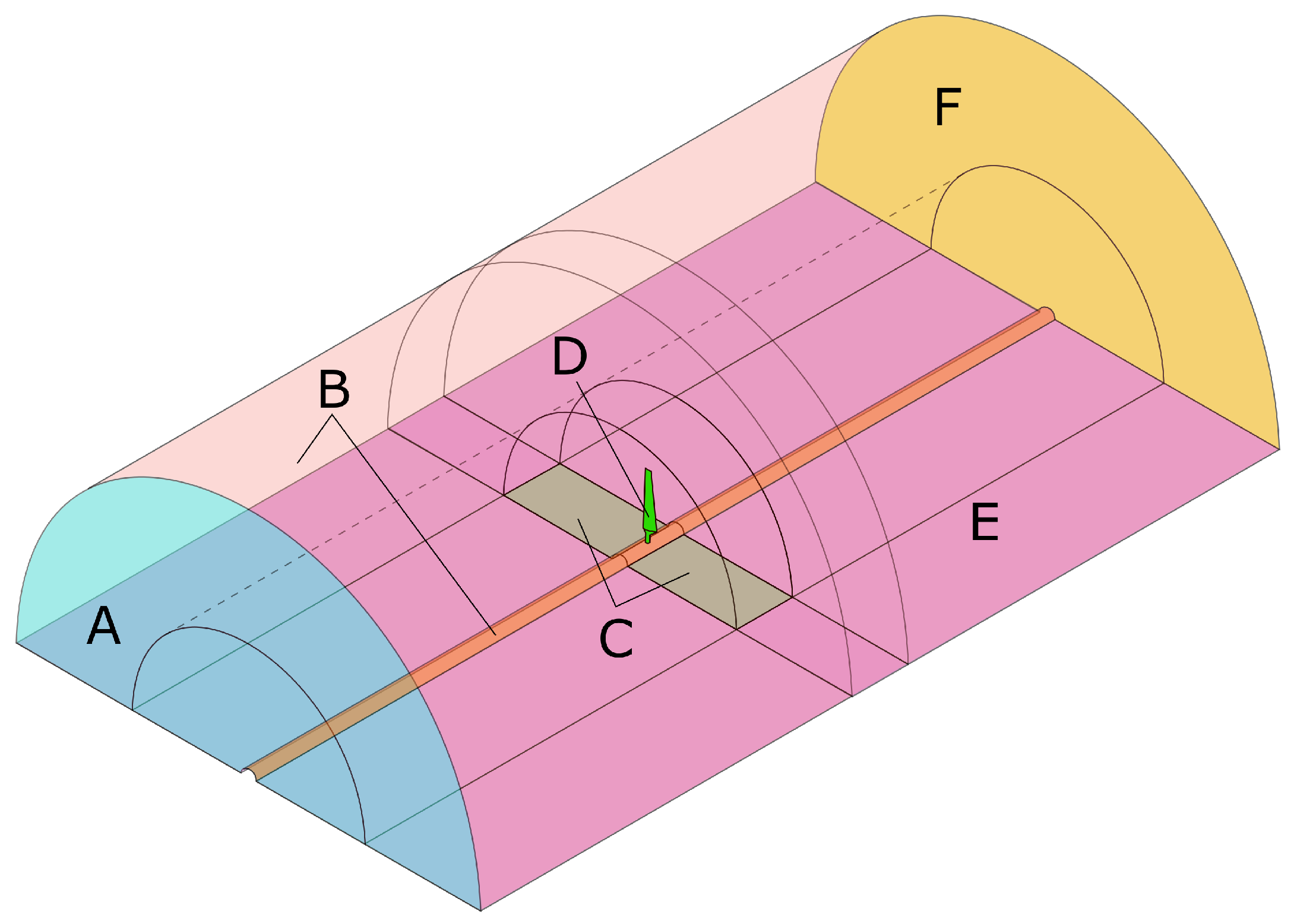
Figure 1. Fluid flow domain and boundary layout; A: velocity inlet, B: slip walls, C: periodic boundaries for sliding mesh, D: no-slip wall, E: periodic boundaries, F: pressure outlet.
Energies 16 06619 g001
Figure 2. Fluid flow domain and mesh details. (a) General mesh layout; (b) Boundary layer inflation.
Energies 16 06619 g002
Figure 3. Structural domain and mesh details. (a) NREL Phase VI blade geometry; (b) Finite-element mesh.
Energies 16 06619 g003
Figure 4. D-spar cross-sectional geometry.
Energies 16 06619 g004
Figure 5. ACC fan blade—fluid-flow domain and boundary layout; G: velocity inlet, H: no-slip blade wall, I: wind tunnel symmetry walls, K: pressure outlet.
Energies 16 06619 g005
Figure 6. Structural concept of the proposed numerical model.
Energies 16 06619 g006
Figure 7. Blade laminate groups and relative positions for one blade shell.
Energies 16 06619 g007
Figure 8. Off-axis fiber orientation for the tailored blade.
Energies 16 06619 g008
Figure 9. Workflow for the simulation plan.
Energies 16 06619 g009
Figure 10. D-spar analysis results [29]. (a) Static deflection in the vertical (flapwise) direction; (b) Longitudinal strain; (c) Twist distribution.
Energies 16 06619 g010
Figure 11. Aerodynamic force validation for the reference case. (a) Lift coefficient curve; (b) Drag coefficient curve [30,32].
Energies 16 06619 g011
Figure 12. Blade tip displacement prediction under base excitation conditions [33].
Energies 16 06619 g012
Figure 13. Structural properties for the baseline blade. (a) Cumulative mass distribution; (b) Flapwise stiffness distribution; (c) Axial stiffness distribution; (d) Torsional stiffness distribution.
Energies 16 06619 g013
Figure 14. Structural properties for the blade with coupling. (a) Cumulative mass distribution; (b) flapwise bending stiffness distribution; (c) Axial stiffness distribution; (d) Torsional stiffness distribution.
Energies 16 06619 g014
Figure 15. Structural responses for reference and coupled blade. (a) flapwise displacement for reference blade in z-axis; (b) flapwise displacement for blade with coupling in z-axis; (c) Torsional deformation for reference blade; (d) Torsional deformation for the blade with coupling.
Energies 16 06619 g015
Figure 16. Coupled simulation results for rotor torque and blade root moment. (a) Low speed shaft torque at different wind speeds; (b) flapwise bending moment at the blade root; (c) Edgewise bending moment at the blade root.
Energies 16 06619 g016
Figure 17. Thrust force and low-speed shaft torque result with blade-element momentum computations. (a) Thrust curve comparison; (b) Power curve comparison.
Energies 16 06619 g017
Figure 18. Flapwise and torsional displacement for the EWM.
Energies 16 06619 g018
Table 1. Main characteristics of relevant works.
Coupling ConceptDeclared TargetFSI InterfaceStructural ModellingStruc. Modelling ToolAerodynamic ModellingAero. Modelling ToolSource
IIncrease of AEP, power regulation.WTABFEMTRICBEMWTAero [15]
PrescribedIncrease in AEP, reduction of loads.N/AN/AN/ABEM, Surface-PanelCwind, Palisupan [16]
I, IIStructural design of blade with aeroelastic tailoring.N/AFEMNASTRANBEMDeveloped by the authors [7]
IReduction of loads.ADAMSFEMHyBladeBEM, Generalized Dynamic Wake ModelAeroDyn [17]
IIIOptimization for max AEP.HAWCStab2FEMHAWCStab2BEMHAWCStab2 [18]
PrescribedReduction of power losses.HAWCStab2FEMHAWCStab2BEMHAWCSTab2 [19]
INumerical modeling with vortex method.FASTFEMBeamDynLifting line free vortex wakeQblade [20]
I, IIAnalysis of power performance, load alleviation, and pitch actuation.DNV GL BladedMulti-body dynamics, modal representationDNV GL Bladed, PreCompBEMDNV GL Bladed [8]
IAnalysis of reduction in damage equivalent loads.PHATASFEMPHATASBEMPHATAS [21]
IOptimization of tow orientation for maximized power output.Partitioned, two-wayFEMABAQUSRANS, k- ε CRUNCH CFD [22]
I, IILoad alleviation.Partitioned, two-wayFEMABAQUSRANS, k- ω SSTSTAR–CCM+ [9]
Table 2. Boundary condition specification at the coupling interface.
Field ProblemSolution MethodBoundary Condition at InterfaceBoundary Value Source
Fluid Flow SolutionFVMNo-slip and no-through condition for velocity (Dirichlet)N/A, fixed by definition ( u , v , w = 0 m / s at the blade surface)
Structural SolutionFEMForce per unit area (von Neumann)Fluid Flow Solution
Mesh DeformationFVMMesh velocity at the boundary (Dirichlet)Structural Solution
Table 3. Simulation cases.
Case NameDescriptionWind Speed in m/sSubjectSystem
Validation cases
VA01D-Spar-D-SparComposite–Structural
VA02ACC fan blade CFD20.45ACC fan bladeFluid flow
VA03ACC fan blade FSI20.45ACC fan bladeFSI
VA04Equivalent neutral blade-Wind turbine bladeStructural
VA05Equivalent coupled blade-Wind turbine bladeStructural
VA06Tip rotation sensitivity study-Wind turbine bladeStructural
Main cases
MC062-way FSI 7N7Neutral bladeSystem Coupling
MC072-way FSI 10N10Neutral bladeSystem Coupling
MC082-way FSI 13N13Neutral bladeSystem Coupling
MC092-way FSI 20N20Neutral bladeSystem Coupling
MC102-way FSI 39N39Neutral bladeSystem Coupling
MC112-way FSI 7C7Coupled bladeSystem Coupling
MC122-way FSI 10C10Coupled bladeSystem Coupling
MC132-way FSI 13C13Coupled bladeSystem Coupling
MC142-way FSI 20C20Coupled bladeSystem Coupling
MC152-way FSI 39C39Coupled bladeSystem Coupling
Auxiliary cases
AX16BEM5 to 25Deformed bladeFluid flow
AX177N CFD7Rigid bladeFluid flow
AX1810N CFD10Rigid bladeFluid flow
AX1913N CFD13Rigid bladeFluid flow
AX2020N CFD20Rigid BladeFluid flow
Table 4. Laminate layup sequences.
Ply GroupPly CountLaminate Sequence
G18 [ 0 ° / 45 ° / 0 ° / 45 ° / 45 ° / 0 ° / 45 ° / 0 ° ]
G21 [ 0 ° / 0 ° ]
G31 [ 0 ° / 0 ° ]
G432 [ ± 45 ° / 0 ° / 90 ° / 45 ° / 0 ° / 0 ° / 45 ° / 0 ° / 90 ° / ± 45 ° / 0 ° / 0 ° ] s
G51 [ 0 ° / 0 ° ]
G61 [ 0 ° / 0 ° ]
G78 [ 0 ° / 45 ° / 0 ° / 45 ° / 45 ° / 0 ° / 45 ° / 0 ° ]
Table 5. Laminate layup sequences for a blade with bend–twist coupling.
Ply GroupPly CountLaminate Sequence
G16 [ θ / 0 ° / θ / θ / 0 ° / θ ]
G21 [ θ ]
G31 [ θ ]
G432 [ θ 2 / 0 ° / 90 ° / θ 6 / 0 ° / 90 ° / θ 4 ] s
G51 [ θ ]
G61 [ θ ]
G76 [ θ / 0 ° / θ / θ / 0 ° / θ ]
Table 6. Load analysis at the blade root.
BladeFlapwise Moment [N m]Edgewise Moment [N m]Torsional Moment [N m]Axial Force [N]Tangential Force [N]
Reference−7214.361375.69288.44−2525.57−545.92
Coupled−7235.301429.58286.52−2530.76−562.32
Disclaimer/Publisher’s Note: The statements, opinions and data contained in all publications are solely those of the individual author(s) and contributor(s) and not of MDPI and/or the editor(s). MDPI and/or the editor(s) disclaim responsibility for any injury to people or property resulting from any ideas, methods, instructions or products referred to in the content.