Robust Nonlinear Control of a Wind Turbine with a Permanent Magnet Synchronous Generator

Abstract

This paper addresses the design of a robust nonlinear dynamic controller for a wind turbine. The turbine is equipped with a permanent magnet synchronous generator. The control problem involves tracking a suitable reference value for the turbine’s angular velocity, which corresponds to the wind speed. This issue is tackled by compensating for variations in the electrical and mechanical parameters present in the mathematical model. Additionally, the problem is approached under the assumption that wind speed cannot be directly measured, a fact verified in practical scenarios. This situation is particularly relevant for real-world applications, where only nominal parameter values are accessible and accurate wind speed measurement is challenging due to disturbances caused by the turbine or other factors, despite the use of appropriate sensors. To achieve precise tracking of the angular velocity reference, effective compensation of perturbation terms arising from parameter uncertainties and errors in wind estimation becomes crucial. To address this problem, a wind velocity estimator is employed in conjunction with high-order sliding mode parameter estimators, ensuring the turbine’s operation attains a high level of performance.

1. Introduction

Wind turbine conversion systems (WTCS) have recently attracted considerable attention from the scientific community. This is due to their potential for renewable energy generation. Thus, the nonlinear control of small and large wind turbines (WTs) is the subject of many works in the literature. In particular, due to their advantages in terms of efficient and reliable operation, permanent magnet synchronous generators (PMSGs) are used as WT generators. These advantages are combined with the features of self-excitation and low speed. These features are integral to direct-drive WTCs. In fact, PMSGs have a simpler mechanical structure and can be directly coupled to the WT shaft, eliminating the need for gears, and they do not require an external excitation system, eliminating the associated copper losses.

The aim is to maximize the amount of power generated by the WT under conditions in which the wind speed is variable. This is achieved by maintaining the so-called tip–speed ratio, i.e., the ratio between the blade tip linear velocity and the wind velocity, at an optimal value. For a given wind speed, this optimum value of the tip–speed ratio corresponds to a certain angular velocity. This is taken as the reference to be tracked. Therefore, the optimal power extraction problem can be expressed as tracking the reference angular velocity corresponding to the given wind speed.

This tracking problem is here solved in the presence of some difficulties that normally arise in practical cases. The first difficulty is that the measurement of the real wind velocity value is unrealistic for industrial WTs. In fact, it is not possible to measure wind speed accurately. Even with the appropriate sensors, the wind velocity field is perturbed by the turbine itself. A second difficulty is that the parameters in the mechanical and electrical equations are usually subject to parameter variations or uncertainties. Examples are the winding resistance, air density, etc., which are subject to variations, and the PMSG rotor inertia, friction, etc., which are known with a certain uncertainty. In practice, only the nominal values of these parameters can be assumed known. In order to solve the tracking problem in the presence of these two difficulties, in this work an estimator of the wind velocity is used. Furthermore, high-order sliding mode (HOSM) estimators are used to estimate the perturbation terms arising in the dynamical equations due to the parameter uncertainties. This allows a compensation of the perturbation terms due to the parameter uncertainties and of the wind estimation error, ensuring an accurate tracking of the reference angular velocity.

Typically, wind speed sensors are mainly installed around the WT to provide wind speed data [1]. The wind speed sensor cannot fully monitor the wind speed at every part of the WT and, therefore, cannot give an accurate wind speed value, as it measures the wind speed at a single point. In addition, the WT wake effect [2] and the tower shadow effect [3] can affect the actual ability of WTs to convert wind energy, reducing the overall efficiency of the wind power system. In addition, the efficiency of the anemometer sensors usually mounted on the top of the WT nacelle, is used to measure the wind speed. Their measurements may be due to the turbulence of the wind and, therefore, may not be representative of the wind speed upstream of the rotor blades. Linear and nonlinear Kalman filter methods can be applied to estimate the effective wind speed [4], along with other methods such as those based on machine learning [5], to reconstruct a spatiotemporal field of wind speed on a regular grid from spatially irregularly distributed measurements and to transform the wind speed to wind power estimates. A widely used approach to overcome the lack of accurate wind speed measurement is the use of the maximum power point tracking (MPPT) technique [6]. This technique is also widely used in solar power systems. This technology optimizes the available wind power by maximizing the electrical output of the turbine.

Regarding parameter variations and uncertainties, the first-order sliding mode (FOSM) technique constitutes an interesting methodology that can be used to compensate for their effects. This is achieved thanks to the inherent robustness of this technique [7]. Examples of FOSM controls of WTs are given in [8,9], which present robust controllers designed for variable speed WTs with doubly fed induction generators. A FOSM control is also designed in [10] for a turbine model considering the mechanical dynamics only, along with a modified Newton–Rapshon algorithm to estimate the wind speed. Another FOSM controller, using the blade pitch as input, was designed in [11] in the presence of uncertainties to regulate the rotor speed to a fixed rated value. A FOSM control for a variable speed WT with a PMSG was considered in [12], under the assumption of measurability of the wind speed. In [13], an algorithm based on the combination of a FOSM and fractional-order sliding mode (SM) was proposed, where the latter ensures finite-time convergence to zero of the angular velocity tracking error. In [14], a novel robust FOSM control was proposed, using nonlinear perturbation observers for WTs with a doubly fed induction generator. Finally, an integral terminal FOSM controller was proposed in [15] to enhance the power quality of WTs under unbalanced voltage conditions.

FOSM control schemes may suffer from the well-known chattering problem, i.e., high-frequency oscillations due to actuator bandwidth limitations, unable to reproduce exactly the sign “function” used in a FOSM, which has clear negative consequences. In order to overcome this difficulty, and to consider SM surfaces with a relative degree greater than one [16], HOSM techniques can be used. These techniques, also called super-twisting (ST) SM techniques, have other appealing properties, since they ensure finite-time convergence to the origin and robustness with respect to perturbation acting on the system. Such techniques were developed starting from the seminal paper of [17] and successively fully developed in successive papers [18,19,20,21,22,23,24]. HOSM techniques were first used for smooth control systems and successively as finite-time differentiators. They were also applied successfully to a number of applications [16,25,26,27,28,29,30,31,32]. Recently, extensive research has been undertaken to control PMSGs for wind energy conversion applications using HOSM techniques. In [33], an efficient controller based on a HOSM was proposed and applied to a PMSG. A HOSM–based control strategy for optimizing the power output of a wind energy conversion system (WECS) with a PMSG was proposed in [34]; this controller incorporates a standalone hybrid system to achieve optimal power conversion and regulation during operational modes. In the works of [35,36], an advanced HOSM control strategy was devised for a PMSG. The proposed approach incorporates a robust aerodynamic torque observer rooted in the ST algorithm, effectively eliminating the need for wind speed measurement sensors. Additionally, a robust control mechanism for WT speed was integrated, aimed at precisely regulating rotor currents. Moreover, in [37], an adaptive sliding mode speed control algorithm was put forth, featuring an integral-operation sliding surface, for a variable speed wind energy experimental system; this controller encompasses an estimator designed to address uncertainties such as the unknown turbine torque and deviations from the mathematical system model, with the ultimate goal of attaining zero steady-state error in the control performance. An adaptive ST approach to control the wind energy conversion system of the PMSG, connected to the electrical system via grid-side and machine-side converters with a capacitor as a DC link between them, was proposed in [38]. Moreover, utilizing an adaptive second-order sliding mode control (SOSMC), in [39], an ST algorithm was examined, with the aim of achieving a robust and rapid current control for WECS based on PMSGs; the primary objective of the controller was to regulate the winding current in order to ensure that the PMSG delivers the desired power to the grid. Further, Ref. [40] presented ST algorithms with a gain adaptation algorithm based on collective/individual blade pitch control, applied to the floating WTs control problem in the above-rated region; the control goals were the regulation of the rotor speed, the reduction in the platform pitch motion, and the reduction in the fatigue load of the blades. A FOSM and a SOSM control scheme based on pulse-width modulation for the rotor-side converter and grid-side converter feeding a doubly fed induction generator (DFIG) were presented in [41,42]. It is worth noticing that all of these works do not deal with parameter uncertainties in the PMSG dynamics.

In this paper, a robust nonlinear dynamic controller is designed for a WT with a PMSG, which guarantees the maximization of the power extracted by the WT from the wind. The control objective is to track an appropriate angular velocity signal, ensuring the asymptotic stability of the closed-loop system despite variations in all the parameters present in the WT mathematical model. The original contributions of this paper are centered around solving the tracking problem in the presence of the following factors:

1.

Unknown wind velocity, which is estimated based on measurements of the produced power.

2.

Parameter variations and uncertainties in the WT model, which are estimated using HOSM estimators.

It is also worth noticing that the unavailability of wind velocity measurement is not considered in the available literature. To address this limitation and establish an angular velocity reference, we employ the MPPT technique, which finds common use in solar power systems and WTs. By optimizing operational parameters, this technique enhances the turbine’s electrical output to harness the highest attainable wind power.

The paper is organized as follows. In Section 2, the mathematical model of a WT is recalled, and the control problem is formulated. In Section 3, a robust nonlinear dynamic controller is presented. In Section 4, the proposed controller is tested via simulations. Some comments conclude the paper.

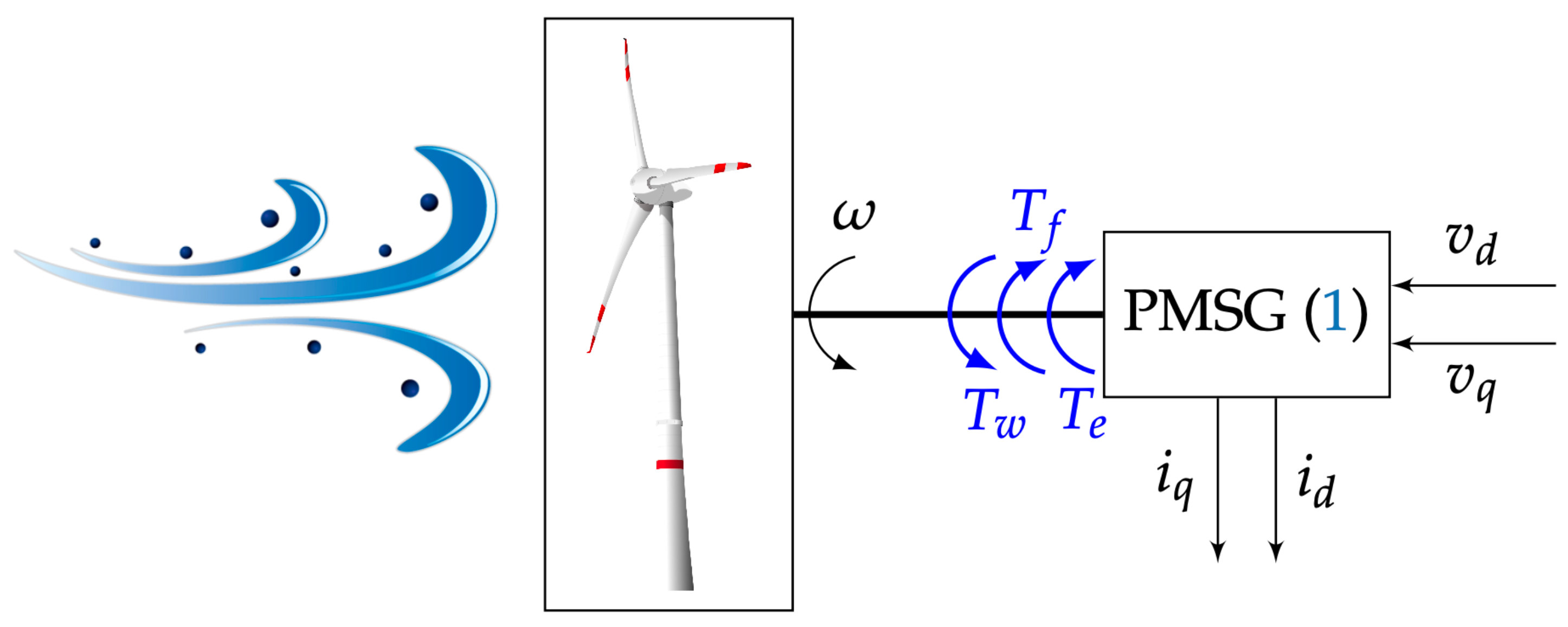
2. Mathematical Model of a WT

The power extracted by the WT from the wind is given by [43]

$$P_w=\frac{1}{2}\varrho \pi R^2{C}_p(\lambda ,\beta )v_w^3=k_w{\omega }^3,k_w=\frac{1}{2}\varrho \pi R^5\frac{C_p(\lambda ,\beta )}{{\lambda }^3}$$

where $\varrho$ is the air density, R is the WT rotor radius, $v_w$ is the wind speed, $\omega$ is the turbine shaft speed, and $\lambda =\omega R/v_w$ is the tip–speed ratio, with $\omega R$ as the tip speed of the turbine blade. Furthermore, $C_p(\lambda ,\beta )$ denotes the power coefficient, contingent upon the specific blade design. This coefficient depends on both the blade pitch angle $\beta$ and the tip–speed ratio $\lambda$, signifying the turbine’s efficacy in transforming the wind’s kinetic energy into mechanical energy. For $\beta ={\beta }^{\circ }=0$, the nonlinear dependency of the power coefficient $C_p$ on $\lambda$ can be approximated by the following experimental expression, as described in [44,45]

$$C_p(\lambda ,{\beta }^{\circ })=c_1\left(c_2\frac{1-c_3\lambda }{\lambda }-c_4\right)e^{-c_5\frac{1-c_3\lambda }{\lambda }}+c_6\lambda$$

where $c_1,\dots ,c_6$ are experimental coefficients depending on the shape of the blade and on its aerodynamic performance.

To maximize the power $P_w$ generated by the WT for a given wind velocity $v_w$, one has to maximize the power coefficient $C_p$. Since this latter depends on $\lambda$ and $\beta$, also its maximum depends on these two variables. Nevertheless, usually $\beta$ is changed occasionally, and in the following it will be considered constant and equal to a value ${\beta }^{\circ }=0$ deg. Therefore, the maximization of $P_w$ is achieved maximizing $C_p(\lambda ,{\beta }^{\circ })$, which has its maximum $C_{p,max}$ for ${\lambda }_{max}$. Obviously, the same reasoning can be followed for other values of the blade pith angle $\beta$.

The model of a PMSG in the $(d,q)$ reference frame, rotating synchronously with the generator rotor, is [45]

$$\begin{array}{cc}\hfill \frac{d{i}_d}{dt}& =-\frac{R_s}{L}{i}_d+p\omega i_q+\frac{1}{L}{v}_d\hfill \\ \hfill \frac{d{i}_q}{dt}& =-\frac{R_s}{L}{i}_q-p\omega i_d-p\frac{{\varphi }_m}{L}\omega +\frac{1}{L}{v}_q\hfill \\ \hfill \dot{\omega }& =-\frac{T_e}{J}-\frac{T_f}{J}+\frac{T_w}{J}=-\frac{k_m}{J}{i}_q-\frac{f}{J}\omega +\frac{k_w}{J}{\omega }^2\hfill \end{array}$$

(1)

where the stator currents $i_d$ and $i_q$ represent the components of the current in the stator projected along the d and q axes, respectively, while $v_d$ and $v_q$ denote the corresponding stator voltage components. Furthermore, the winding resistance and inductance are denoted by $R_s$ and $L=L_d=L_q$, respectively. The flux linkage of the permanent magnet is symbolized as ${\psi }_m$, and the electrical angular speed ${\omega }_e$ of the generator rotor is equal to $p\omega$, where p denotes the number of pole pairs. The mechanical equation is obtained considering the external torques given by the electrical torque, the viscous friction torque $T_f$, and the torque $T_w$ extracted from the wind. The electrical torque is given by $T_e=k_m{i}_q$, where $k_m=3p{\varphi }_m/2$ represents the torque constant, and the generated motor torque is proportional to the current $i_q$, grounded in the assumption of the absence of a reluctance torque in the considered PMSG. Moreover, the mechanical inertia is indicated by J, while $T_f=f\omega$ denotes the viscous friction torque, with f the viscous friction coefficient. The torque $T_w$ harnessed from the wind is determined as $P_w/\omega$ or equivalently $k_w{\omega }^2$. The parameter $k_w$ encapsulates the influence of the aerodynamic torque and is a parameter that is generally known with great inaccuracy. The scheme of a WT with a PMSG is depicted in Figure 1.

In this work, all of the parameters appearing in the electric and mechanical dynamics (1) are assumed to be subject to variation. Let $R_s^{\circ }$, $L^{\circ }$, ${\varphi }_m^{\circ }$, $k_m^{\circ }=3p{\varphi }_m^{\circ }/2$, $J^{\circ }$, $f^{\circ }$ be the nominal values of $R_s$, L, ${\varphi }_m$, $k_m$, J, f, and

$$k_w^{\circ }=\frac{1}{2}{\varrho }^{\circ }\pi {\left(R^{\circ }\right)}^5\frac{C_p^{\circ }({\lambda }^{\circ },{\beta }^{\circ })}{{\left({\lambda }^{\circ }\right)}^3}$$

the nominal value of $k_w$, where ${\varrho }^{\circ }$ is the nominal value of $\varrho$, $R^{\circ }$ is the nominal value for R, ${\lambda }^{\circ }=\omega R^{\circ }/v_w$, and $C_p^{\circ }$ is the nominal function

$$C_p^{\circ }({\lambda }^{\circ },{\beta }^{\circ })=c_1^{\circ }\left(c_2^{\circ }\frac{1-c_3^{\circ }{\lambda }^{\circ }}{{\lambda }^{\circ }}-c_4^{\circ }\right)e^{-c_5^{\circ }\frac{1-c_3^{\circ }{\lambda }^{\circ }}{{\lambda }^{\circ }}}+c_6^{\circ }{\lambda }^{\circ }$$

with $c_1^{\circ },\dots ,c_6^{\circ }$, use the nominal values of $c_1,\dots ,c_6$. Finally, the nominal value of $T_w$ is $T_w^{\circ }=k_w^{\circ }{\omega }^2$.

In what follows, it will be assumed that the parameter variations $|R_s-R_s^{\circ }|$, $|L-L^{\circ }|$, $|{\varphi }_m-{\varphi }_m^{\circ }|$, $|J-J^{\circ }|$, $|f-f^{\circ }|$, $|\varrho -{\varrho }^{\circ }|$, and $|R-R^{\circ }|$ are bounded by certain values ${∆}_{R_s}$, ${∆}_L$, ${∆}_{{\varphi }_m}$, ${∆}_J$, ${∆}_f$, ${∆}_{\varrho }$, and ${∆}_R$, respectively. This is an acceptable assumption from a physical point of view.

The control problem consists of designing a dynamic controller to track a reference angular velocity ${\omega }_{\mathrm{ref}}$, which will be determined later, in the presence of uncertainties on all the parameters appearing in the model.

Considering the maximization of $P_w$, which is obtained by imposing the value ${\lambda }_{max}$ and using the definition of the tip–speed ratio, one obtains the reference angular velocity ${\lambda }_{max}{v}_w/R$, that should be imposed. However, one observes that such a function is unknown, as ${\lambda }_{max}$ and $v_w$ are unknown. Therefore, in the following, an estimation of the wind velocity will be determined, while ${\lambda }_{max}$ will be substituted by its (known) nominal value ${\lambda }_{max}^{\circ }$.

3. Design of the Dynamic Controller for the Tracking of the Angular Velocity Reference

The initial step in designing the desired controller involves estimating the wind velocity to establish a known angular velocity reference. For this purpose, we employ the MPPT technique, commonly used in solar power systems and WTs. In the context of WTs, MPPT optimizes the turbine’s electrical output by adjusting operational parameters to capture the maximum available wind power. As wind conditions continually fluctuate in speed and direction, a WT’s power generation varies accordingly. The MPPT system constantly monitors these conditions, adapting the turbine’s electrical load and rotational speed to operate at the point of maximum wind power extraction. In this work, the MPPT technique is employed to establish the angular velocity reference [6]. Once the reference angular velocity is determined, the controller will be designed to impose such a reference.

3.1. Design of the Wind Velocity Estimator

As already commented, the measurement of the real velocity value $v_w$ is unrealistic for industrial WTs. In the following, the wind velocity $v_w$ can be estimated from the measurement of the produced power $P_m$. In fact, considering the nominal value $k_w^{\circ }$ and the function

$$f\left({\lambda }^{\circ }\right)=P_m-k_w^{\circ }{\omega }^3=P_m-\frac{1}{2}{\varrho }^{\circ }\pi {\left(R^{\circ }\right)}^5\frac{C_p^{\circ }({\lambda }^{\circ },{\beta }^{\circ })}{{\left({\lambda }^{\circ }\right)}^3}{\omega }^3$$

it is possible to determine the value of ${\lambda }^{\circ }$ by imposing $f\left({\lambda }^{\circ }\right)=0$. To this aim, among the other methods, a Newton–Raphson method can be used [6]. Hence, one can look for the solution’s $\widehat{\lambda }$ of the equation $f\left({\lambda }^{\circ }\right)=0$ considering the iterative estimations

$${\lambda }_k^{\circ }={\lambda }_{k-1}^{\circ }-\frac{f\left({\lambda }^{\circ }\right)}{f^{\prime }\left({\lambda }^{\circ }\right)}{|}_{{\lambda }^{\circ }={\lambda }_{k-1}^{\circ }},k=1,2,\dots ,N$$

for a fixed integer $N\in \mathbb{Z}$, where

$$f^{\prime }\left({\lambda }^{\circ }\right)=-\frac{1}{2}{\varrho }^{\circ }\pi {\left(R^{\circ }\right)}^5{\omega }^3\frac{d(C_p^{\circ }({\lambda }^{\circ },{\beta }^{\circ })/{\left({\lambda }^{\circ }\right)}^3)}{d{\lambda }^{\circ }}.$$

From the definition of ${\lambda }^{\circ }$, and using the estimation of $\widehat{\lambda }$, one computes the wind velocity estimation

$${\widehat{v}}_w=\frac{R^{\circ }}{\widehat{\lambda }}\omega$$

(2)

and the following reference angular velocity

$${\omega }_{\mathrm{ref}}=\frac{{\lambda }_{max}^{\circ }}{R^{\circ }}{\widehat{v}}_w=\frac{{\lambda }_{max}^{\circ }}{\widehat{\lambda }}\omega$$

(3)

can be defined, with ${\lambda }_{max}^{\circ }$ as the (known) maximum value of $C_p^{\circ }({\lambda }^{\circ },{\beta }^{\circ })$. This is the reference angular velocity that the controller has to track in the presence of parameter uncertainties.

3.2. Design of the Dynamic Controller for the Tracking of the Angular Velocity Reference

Given model (1) and considering the nominal values $R_s^{\circ }$, $L^{\circ }$, ${\varphi }_m^{\circ }$, $k_m^{\circ }$, $f^{\circ }$, $k_w^{\circ }$, one obtains the following model

$$\begin{array}{cc}\hfill \frac{d{i}_d}{dt}& =-\frac{R_s^{\circ }}{L^{\circ }}{i}_d+p\omega i_q+\frac{1}{L^{\circ }}{v}_d+{∆}_1\hfill \\ \hfill \frac{d{i}_q}{dt}& =-\frac{R_s^{\circ }}{L^{\circ }}{i}_q-p\omega i_d-p\frac{{\varphi }_m^{\circ }}{L^{\circ }}\omega +\frac{1}{L^{\circ }}{v}_q+{\delta }_2\hfill \\ \hfill \dot{\omega }& =-\frac{k_m^{\circ }}{J^{\circ }}{i}_q-\frac{f^{\circ }}{J^{\circ }}\omega +\frac{k_w^{\circ }}{J^{\circ }}{\omega }^2+{∆}_3\hfill \end{array}$$

(4)

with the perturbation terms

$$\begin{array}{cc}\hfill {∆}_1& =-\left(\frac{R_s}{L}-\frac{R_s^{\circ }}{L^{\circ }}\right)i_d+\left(\frac{1}{L}-\frac{1}{L^{\circ }}\right)v_d\hfill \\ \hfill {\delta }_2& =-\left(\frac{R_s}{L}-\frac{R_s^{\circ }}{L^{\circ }}\right)i_q-p\left(\frac{{\varphi }_m}{L}-\frac{{\varphi }_m^{\circ }}{L^{\circ }}\right)\omega +\left(\frac{1}{L}-\frac{1}{L^{\circ }}\right)v_q\hfill \\ \hfill {∆}_3& =-\left(\frac{k_m}{J}-\frac{k_m^{\circ }}{J^{\circ }}\right)i_q-\left(\frac{f}{J}-\frac{f^{\circ }}{J^{\circ }}\right)\omega +\left(\frac{k_w}{J}-\frac{k_w^{\circ }}{J^{\circ }}\right){\omega }^2.\hfill \end{array}$$

The final perturbation term ${∆}_2$ for the dynamics of $i_q$ will be given by the sum of ${\delta }_2$ and additional terms arising from the derivative of the reference imposed on $i_q$. This will become clearer in the subsequent computations.

The following result solves the posed control problem for system (4).

Theorem 1.

If the signals $i_d$, $i_q$, ω are measurable, the dynamic controller

$$\begin{array}{cc}\hfill {\dot{\xi }}_{1,1}& =-\frac{R^{\circ }}{L^{\circ }}{i}_d+p\omega i_q+\frac{1}{L^{\circ }}{v}_d-{\alpha }_{1,1}{⌊{\xi }_{1,1}-(i_d-i_{d,\mathrm{ref}})⌉}^{1/2}+{\xi }_{1,2}\hfill \\ \hfill {\dot{\xi }}_{1,2}& =-{\alpha }_{1,2}{⌊{\xi }_{1,1}-(i_d-i_{d,\mathrm{ref}})⌉}^0\hfill \\ \hfill {\dot{\xi }}_{2,1}& =-\frac{R^{\circ }}{L^{\circ }}{i}_q-p\omega i_d-p\frac{{\varphi }_m^{\circ }}{L^{\circ }}\omega +\frac{1}{L^{\circ }}{v}_q-D_{i_{q,\mathrm{ref}}}^{\circ }-{\alpha }_{2,1}{⌊{\xi }_{2,1}-(i_q-i_{q,\mathrm{ref}})⌉}^{1/2}+{\xi }_{2,2}\hfill \\ \hfill {\dot{\xi }}_{2,2}& =-{\alpha }_{2,2}{⌊{\xi }_{2,1}-(i_q-i_{q,\mathrm{ref}})⌉}^0\hfill \\ \hfill {\dot{\xi }}_{3,1}& =c\left(-\frac{k_m^{\circ }}{J^{\circ }}{i}_q-\frac{f^{\circ }}{J^{\circ }}\omega +\frac{k_w^{\circ }}{J^{\circ }}{\omega }^2\right)-{\alpha }_{3,1}{⌊{\xi }_{3,1}-(\omega -{\omega }_{\mathrm{ref}})⌉}^{1/2}+c{\xi }_{3,2}\hfill \\ \hfill {\dot{\xi }}_{3,2}& =-\frac{{\alpha }_{3,2}}{c}{⌊{\xi }_{3,1}-(\omega -{\omega }_{\mathrm{ref}})⌉}^0\hfill \\ \hfill {\dot{I}}_{e_{i_d}}& =i_d-i_{d,\mathrm{ref}}\hfill \\ \hfill {\dot{I}}_{e_{i_q}}& =i_q-i_{q,\mathrm{ref}}\hfill \\ \hfill {\dot{I}}_{e_{\omega }}& =\omega -{\omega }_{\mathrm{ref}}\hfill \\ \hfill v_d& =L^{\circ }\left(-k_{1,p}(i_d-i_{d,\mathrm{ref}})-k_{1,i}{I}_{e_{i_d}}+\frac{R_s^{\circ }}{L^{\circ }}{i}_d-p\omega i_q+\frac{d}{dt}{i}_{d,\mathrm{ref}}-{\xi }_{1,2}\right)\hfill \\ \hfill v_q& =L^{\circ }\left(-k_{2,p}(i_q-i_{q,\mathrm{ref}})-k_{2,i}{I}_{e_{i_q}}+\frac{R_s^{\circ }}{L^{\circ }}{i}_q+p\omega i_d+p\frac{{\varphi }_m^{\circ }}{L^{\circ }}\omega +D_{i_{q,\mathrm{ref}}}^{\circ }-{\xi }_{2,2}\right)\hfill \end{array}$$

(5)

where ${⌊·⌉}^{\alpha }={|·|}^{\alpha }\mathrm{sign}(·)$, with $c=1-{\lambda }_{max}^{\circ }/\widehat{\lambda }$, $k_{j,p},k_{j,i}>0$, $j=1,2,3$, and

$$\begin{array}{cccc}\hfill {\alpha }_{1,1}& >0,\hfill & \hfill {\alpha }_{1,2}& >2\frac{{\theta }_1^2}{{\alpha }_{1,1}^2}+3{\theta }_1\hfill \\ \hfill {\alpha }_{2,1}& >0,\hfill & \hfill {\alpha }_{2,2}& >2\frac{{\theta }_2^2}{{\alpha }_{2,1}^2}+3{\theta }_2\hfill \\ \hfill {\alpha }_{3,1}& >0,\hfill & \hfill {\alpha }_{3,2}& >2\frac{c^2{\theta }_3^2}{{\alpha }_{3,1}^2}+3c{\theta }_3\hfill \end{array}$$

(6)

For some finite positive reals ${\theta }_i$, $i=1,2,3$, ${\omega }_{\mathrm{ref}}$ given by (3),

$$\begin{array}{cc}\hfill i_{d,\mathrm{ref}}& =\phi \left(t\right)\hfill \\ \hfill i_{q,\mathrm{ref}}& =\frac{J^{\circ }}{k_m^{\circ }}\left(\frac{k_{3,p}}{c}(\omega -{\omega }_{\mathrm{ref}})+\frac{k_{3,i}}{c}{I}_{e_{\omega }}+{\xi }_{3,2}-\frac{f^{\circ }}{J^{\circ }}\omega +\frac{k_w^{\circ }}{J^{\circ }}{\omega }^2\right)\hfill \end{array}$$

(7)

where $\phi \left(t\right)$ is a bounded function with a bounded derivative, and

$$\begin{array}{cc}\hfill D_{i_{q,\mathrm{ref}}}^{\circ }& =\frac{J^{\circ }}{k_m^{\circ }}[\frac{k_{3,p}}{c}\left(-\frac{k_m^{\circ }}{J^{\circ }}c{e}_{i_q}-k_{3,p}{e}_{\omega }-k_{3,i}{I}_{e_{\omega }}-c{\xi }_{3,2}\right)\hfill \\ \hfill & +\frac{k_{3,i}}{c}{e}_{\omega }-\frac{{\alpha }_{3,2}}{c}{⌊e_{3,1}⌉}^0+\left(2\frac{k_w^{\circ }}{J^{\circ }}\omega -\frac{f^{\circ }}{J^{\circ }}\right)\left(-\frac{k_m^{\circ }}{J^{\circ }}{i}_q-\frac{f^{\circ }}{J^{\circ }}\omega +\frac{k_w^{\circ }}{J^{\circ }}{\omega }^2\right)]\hfill \\ \hfill D_{i_{q,\mathrm{ref}}}& =\frac{J^{\circ }}{k_m^{\circ }}\left(\frac{k_{3,p}}{c}c+2\frac{k_w^{\circ }}{J^{\circ }}\omega -\frac{f^{\circ }}{J^{\circ }}\right){∆}_3\hfill \end{array}$$

(8)

ensures that the tracking error $\omega -{\omega }_{\mathrm{ref}}$ converges to zero asymptotically. Moreover, the errors $i_d-i_{d,\mathrm{ref}}$, $i_q-i_{q,\mathrm{ref}}$ converge asymptotically to zero.

Proof. 

Let us define the angular velocity tracking error $e_{\omega }=\omega -{\omega }_{\mathrm{ref}}=c\omega$. The dynamics of $e_{\omega }$ are

$$\begin{array}{cc}\hfill {\dot{e}}_{\omega }& =c\dot{\omega }=c\left(-\frac{k_m^{\circ }}{J^{\circ }}{i}_q-\frac{f^{\circ }}{J^{\circ }}\omega +\frac{k_w^{\circ }}{J^{\circ }}{\omega }^2+{∆}_3\right)\hfill \\ \hfill & =c\left(-\frac{k_m^{\circ }}{J^{\circ }}{e}_{i_q}-\frac{k_m^{\circ }}{J^{\circ }}{i}_{q,\mathrm{ref}}-\frac{f^{\circ }}{J^{\circ }}\omega +\frac{k_w^{\circ }}{J^{\circ }}{\omega }^2+{∆}_3\right)\hfill \\ \hfill & =-\frac{k_m^{\circ }}{J^{\circ }}c{e}_{i_q}-k_{3,p}{e}_{\omega }-k_{3,i}{I}_{e_{\omega }}-e_{3,2}\hfill \end{array}$$

(9)

where $e_{i_q}=i_q-i_{q,\mathrm{ref}}$, with $i_{q,\mathrm{ref}}$ as in (7) and $e_{3,2}=c({\xi }_{3,2}-{∆}_3)$. The dynamics of $e_{i_q}$ are

$$\begin{array}{cc}\hfill {\dot{e}}_{i_q}& =-\frac{R_s}{L}{i}_q-p\omega i_d-p\frac{{\varphi }_m}{L}\omega +\frac{1}{L}{v}_q-\frac{d{i}_{q,\mathrm{ref}}}{dt}\hfill \\ & =-\frac{R_s^{\circ }}{L^{\circ }}{i}_q-p\omega i_d-p\frac{{\varphi }_m^{\circ }}{L^{\circ }}\omega +\frac{1}{L^{\circ }}{v}_q+{\delta }_2-D_{i_{q,\mathrm{ref}}}^{\circ }-D_{i_{q,\mathrm{ref}}}\hfill \\ & =-\frac{R_s^{\circ }}{L^{\circ }}{i}_q-p\omega i_d-p\frac{{\varphi }_m^{\circ }}{L^{\circ }}\omega +\frac{1}{L^{\circ }}{v}_q-D_{i_{q,\mathrm{ref}}}^{\circ }+{∆}_2\hfill \end{array}$$

with the derivative of $i_{q,\mathrm{ref}}$ given by

$$\begin{array}{cc}\hfill \frac{d}{dt}{i}_{q,\mathrm{ref}}& =\frac{J^{\circ }}{k_m^{\circ }}\left(\frac{k_{3,p}}{c}{\dot{e}}_{\omega }+\frac{k_{3,i}}{c}{e}_{\omega }+{\dot{\xi }}_{3,2}+\left(2\frac{k_w^{\circ }}{J^{\circ }}\omega -\frac{f^{\circ }}{J^{\circ }}\right)\dot{\omega }\right)=D_{i_{q,\mathrm{ref}}}^{\circ }+D_{i_{q,\mathrm{ref}}}\hfill \end{array}$$

where $D_{i_{q,\mathrm{ref}}}^{\circ }$, $D_{i_{q,\mathrm{ref}}}$ are as in (8), and with the (unknown) perturbation term ${∆}_2$ given by

$$\begin{array}{cc}\hfill {∆}_2& ={\delta }_2-D_{i_{q,\mathrm{ref}}}=-\left(\frac{R_s}{L}-\frac{R_s^{\circ }}{L^{\circ }}\right)i_q-p\left(\frac{{\varphi }_m}{L}-\frac{{\varphi }_m^{\circ }}{L^{\circ }}\right)\omega +\left(\frac{1}{L}-\frac{1}{L^{\circ }}\right)v_q\hfill \\ & +\frac{J^{\circ }}{k_m^{\circ }}\left(\frac{k_{3,p}}{c}c+2\frac{k_w^{\circ }}{J^{\circ }}\omega -\frac{f^{\circ }}{J^{\circ }}\right)\left[\left(\frac{k_m}{J}-\frac{k_m^{\circ }}{J^{\circ }}\right)i_q+\left(\frac{f}{J}-\frac{f^{\circ }}{J^{\circ }}\right)\omega -\left(\frac{k_w}{J}-\frac{k_w^{\circ }}{J^{\circ }}\right){\omega }^2\right].\hfill \end{array}$$

Using controller (5), one works out

$${\dot{e}}_{i_q}=-k_{2,p}{e}_{i_q}-k_{2,i}{I}_{e_{i_d}}-e_{2,2}$$

(10)

with $e_{2,2}={\xi }_{2,2}-{∆}_2$. Considering (9) and (10), one finally obtains the coupled dynamics

$$\begin{array}{c}\left(\begin{array}{c}{\dot{I}}_{e_{\omega }}\hfill \\ {\dot{e}}_{\omega }\hfill \end{array}\right)=\left(\begin{array}{cc}0& 1\\ -k_{3,i}& -k_{3,p}\end{array}\right)\left(\begin{array}{c}{I}_{e_{\omega }}\\ e_{\omega }\end{array}\right)-\left(\begin{array}{cc}0& 0\\ 0& \frac{k_m^{\circ }}{J^{\circ }}c\end{array}\right)\left(\begin{array}{c}{I}_{e_{i_q}}\hfill \\ e_{i_q}\hfill \end{array}\right)-\left(\begin{array}{cc}0\hfill & 0\hfill \\ 0\hfill & 1\hfill \end{array}\right)\left(\begin{array}{c}{e}_{3,1}\hfill \\ e_{3,2}\hfill \end{array}\right)\hfill \\ \left(\begin{array}{c}{\dot{I}}_{e_{i_q}}\hfill \\ {\dot{e}}_{i_q}\hfill \end{array}\right)=\left(\begin{array}{cc}0& 1\\ -k_{2,i}& -k_{2,p}\end{array}\right)\left(\begin{array}{c}{I}_{e_{i_q}}\hfill \\ e_{i_q}\hfill \end{array}\right)-\left(\begin{array}{cc}0\hfill & 0\hfill \\ 0\hfill & 1\hfill \end{array}\right)\left(\begin{array}{c}{e}_{2,1}\hfill \\ e_{2,2}\hfill \end{array}\right)\hfill \end{array}$$

(11)

where the dynamics of the errors $e_{3,1}$, $e_{3,2}$, $e_{2,1}$, $e_{2,2}$, are

$$\begin{array}{cc}\hfill {\dot{e}}_{3,1}& =-{\alpha }_{3,1}{⌊e_{3,1}⌉}^{1/2}+e_{3,2}\hfill \\ \hfill {\dot{e}}_{3,2}& =-{\alpha }_{3,2}{⌊e_{3,1}⌉}^0-c{\dot{∆}}_3\hfill \\ \hfill {\dot{e}}_{2,1}& =-{\alpha }_{2,1}{⌊e_{2,1}⌉}^{1/2}+e_{2,2}\hfill \\ \hfill {\dot{e}}_{2,2}& =-{\alpha }_{2,2}{⌊e_{2,1}⌉}^0-{\dot{∆}}_2.\hfill \end{array}$$

(12)

The errors $e_{3,1}$, $e_{3,2}$ tend to zero in finite time. The proof of the global convergence to the origin in finite time of $e_{3,1}$, $e_{3,2}$ can be demonstrated with Lyapunov arguments [46,47], considering the Lyapunov candidate

$$V_3=\frac{1}{2}{E}_3^T{P}_3{E}_3,P_3=\left(\begin{array}{cc}{\alpha }_{3,1}^2+4{\alpha }_{3,2}& -{\alpha }_{3,1}\\ -{\alpha }_{3,1}& 2\end{array}\right)=P_3^T>0,E_3=\left(\begin{array}{c}{⌊e_{3,1}⌉}^{1/2}\\ e_{3,2}\end{array}\right).$$

This candidate is continuous but not differentiable. As explained in [46], the use of the classical version of Lyapunov’s theory [48], instead of nonsmooth versions [49,50], is allowed since $V_3$ is differentiable almost everywhere, i.e., except when $e_{3,1}=0$. The fact that the trajectories of (12) may pass through $e_{3,1}=0$ for time instants constituting a set of null measures before reaching the origin from a certain finite-time instant allows for use of the classical version of Lyapunov’s theory. Therefore, considering the necessary modifications with respect to the proof given in [46]

$${\dot{V}}_3=-\frac{{\alpha }_{3,1}}{2|e_{3,1}{|}^{1/2}}{E}_3^T{Q}_{3,1}{E}_3-\frac{c{\dot{∆}}_3}{2|e_{3,1}{|}^{1/2}}{⌊e_{3,1}⌉}^0{E}_3^T{Q}_{3,0}{E}_3$$

where

$$\begin{array}{c}{Q}_{3,1}=\frac{P_3{\Lambda }_{3,1}+{\Lambda }_{3,1}^T{P}_3}{2{\alpha }_{3,1}}=\left(\begin{array}{cc}{\alpha }_{3,1}^2+2{\alpha }_{3,2}& -{\alpha }_{3,1}\\ -{\alpha }_{1,1}& 1\end{array}\right)\hfill \\ Q_{3,0}=P_3{\Lambda }_{3,0}=\left(\begin{array}{cc}-2{\alpha }_{3,1}& 2\\ 2& 0\end{array}\right).\hfill \end{array}$$

We will prove later that, with the proposed controller, ${\dot{∆}}_3$ remains bounded, with $|{\dot{∆}}_3|\le {\theta }_3$ for all time instants. To take into account the perturbation ${\dot{∆}}_3$, ${\dot{V}}_3$ can be bounded as follows

$$\begin{array}{cc}\hfill {\dot{V}}_3& \le -\frac{{\alpha }_{3,1}}{2|e_{3,1}{|}^{1/2}}{\mathcal{E}}_3^T{Q}_{3,1}{\mathcal{E}}_3-\frac{c{\theta }_3}{2|e_{3,1}{|}^{1/2}}{\mathcal{E}}_3^T{Q}_{3,0}{\mathcal{E}}_3=-\frac{{\alpha }_{3,1}}{2|e_{3,1}{|}^{1/2}}{\mathcal{E}}_3^T{Q}_3{\mathcal{E}}_3\hfill \\ & \le -\frac{{\alpha }_{3,1}}{2|e_{3,1}{|}^{1/2}}{\lambda }_{min}^{Q_3}{\parallel E_3\parallel }_2^2\le -{\gamma }_3{V}_3^{1/2},{\gamma }_3={\alpha }_{3,1}\frac{\sqrt{{\lambda }_{min}^{P_3}}}{\sqrt{2}{\lambda }_{max}^{P_3}}{\lambda }_{min}^{Q_3}\hfill \end{array}$$

$$\begin{array}{c}{\mathcal{E}}_3=\left(\begin{array}{c}{|⌊e_{3,1}⌉}^{1/2}\mid \\ \left|e_{3,2}\right|\end{array}\right),Q_3=\left(\begin{array}{cc}{\alpha }_{3,1}^2+2{\alpha }_{3,2}-2c{\theta }_3& -\left({\alpha }_{3,1}+\frac{2c{\theta }_3}{{\alpha }_{3,1}}\right)\\ -\left({\alpha }_{3,1}+\frac{2c{\theta }_3}{{\alpha }_{3,1}}\right)& 1\end{array}\right)\hfill \end{array}$$

with ${\alpha }_{3,1}>0,Q_3>0$ under the conditions of (6), and ${∥{\mathcal{E}}_3∥}_2^2={∥E_3∥}_2^2={\left|{⌊e_{3,1}⌉}^{1/2}\right|}^2+{\left|e_{3,2}\right|}^2=\left|e_{3,1}\right|+e_{3,2}^2$. Additionally, here, slight modifications with respect to the proof of [46] were necessary. This proves the finite-time convergence of $E_3$ to the origin.

With the same arguments, the errors $e_{2,1}$, $e_{2,2}$ can also be proved to tend to zero in finite time, considering the Lyapunov candidate

$$V_2=\frac{1}{2}{E}_2^T{P}_2{E}_2,P_2=\left(\begin{array}{cc}{\alpha }_{2,1}^2+4{\alpha }_{2,2}& -{\alpha }_{2,1}\\ -{\alpha }_{2,1}& 2\end{array}\right),E_2=\left(\begin{array}{c}{⌊e_{2,1}⌉}^{1/2}\\ e_{2,2}\end{array}\right).$$

(13)

Moreover, in this case it will be shown that ${\dot{∆}}_2$ remains bounded, with $|{\dot{∆}}_2|\le {\theta }_2$.

Since $e_{2,1}$, $e_{2,2}$, $e_{3,1}$, $e_{3,2}$ tend to zero in finite time, the tracking error dynamics in (11) have the origin globally asymptotically stable, i.e., $e_{\omega }$, $I_{e_{\omega }}$, $e_{i_q}$, $I_{e_{i_q}}$ tend to zero asymptotically.

Finally, considering the expression of the reference $i_{d,\mathrm{ref}}$ as in (7) and the control $v_d$ as in (5), for the error $e_{i_d}=i_d-i_{d,\mathrm{ref}}$, one obtains

$$\begin{array}{cc}\hfill {\dot{e}}_{i_d}& =-\frac{R_s}{L}{i}_d+p\omega i_q+\frac{1}{L}{v}_d-\frac{d}{dt}{i}_{d,\mathrm{ref}}\hfill \\ \hfill & =-\frac{R_s^{\circ }}{L^{\circ }}{i}_d+p\omega i_q+\frac{1}{L^{\circ }}{v}_d-\frac{d}{dt}{i}_{d,\mathrm{ref}}{+}_1\hfill \\ \hfill & =-k_{1,p}{e}_{i_d}-k_{1,i}{I}_{e_{i_d}}-e_{1,2}\hfill \end{array}$$

(14)

where

$$\begin{array}{cc}\hfill {\dot{e}}_{1,1}& =-{\alpha }_{1,1}{⌊e_{1,1}⌉}^{1/2}+e_{1,2}\hfill \\ \hfill {\dot{e}}_{1,2}& =-{\alpha }_{1,2}{⌊e_{1,1}⌉}^0-{\dot{∆}}_1.\hfill \end{array}$$

(15)

With the same arguments used before, $e_{1,1}$, $e_{1,2}$ tend to zero in finite time, since $|{\dot{∆}}_1|\le {\theta }_1$. As a consequence, the closed-loop dynamics

$$\left(\begin{array}{c}{\dot{I}}_{e_{i_d}}\\ {\dot{e}}_{i_d}\end{array}\right)=\left(\begin{array}{cc}0& 1\\ -k_{1,i}& -k_{1,p}\end{array}\right)\left(\begin{array}{c}{I}_{e_{i_d}}\\ e_{i_d}\end{array}\right)-\left(\begin{array}{cc}0\hfill & 0\hfill \\ 0\hfill & 1\hfill \end{array}\right)\left(\begin{array}{c}{e}_{1,1}\hfill \\ e_{1,2}\hfill \end{array}\right)$$

have the origin globally asymptotically stable, i.e., $e_{i_d}$, $I_{e_{i_d}}$ tend to zero asymptotically.

We can now show what was stated before, namely that ${\dot{∆}}_1,{\dot{∆}}_2,{\dot{∆}}_3$ remain bounded for all time instants. In fact, since the initial tracking errors $e_{i_d}\left(0\right)$, $e_{i_q}\left(0\right)$, $e_{\omega }\left(0\right)$ are finite, so are

$$\begin{array}{cc}\hfill {∆}_1\left(0\right)& =-\left(\frac{R_s}{L}-\frac{R_s^{\circ }}{L^{\circ }}\right)i_d\left(0\right)+\left(\frac{1}{L}-\frac{1}{L^{\circ }}\right)v_d\left(0\right)\hfill \\ \hfill {∆}_2\left(0\right)& =-\left(\frac{R_s}{L}-\frac{R_s^{\circ }}{L^{\circ }}\right)i_q\left(0\right)-p\left(\frac{{\varphi }_m}{L}-\frac{{\varphi }_m^{\circ }}{L^{\circ }}\right)\omega +\left(\frac{1}{L}-\frac{1}{L^{\circ }}\right)v_q\left(0\right)-D_{i_{q,\mathrm{ref}}}\left(0\right)\hfill \\ \hfill {∆}_3\left(0\right)& =-\left(\frac{k_m}{J}-\frac{k_m^{\circ }}{J^{\circ }}\right)i_q\left(0\right)-\left(\frac{f}{J}-\frac{f^{\circ }}{J^{\circ }}\right)\omega \left(0\right)+\left(\frac{k_w}{J}-\frac{k_w^{\circ }}{J^{\circ }}\right){\omega }^2\left(0\right)\hfill \end{array}$$

and

$$\begin{array}{cc}\hfill {\dot{∆}}_1\left(0\right)& =-\left(\frac{R_s}{L}-\frac{R_s^{\circ }}{L^{\circ }}\right)\frac{d{i}_d}{dt}{|}_{t=0}+\left(\frac{1}{L}-\frac{1}{L^{\circ }}\right){\dot{v}}_d{|}_{t=0}\hfill \\ \hfill {\dot{∆}}_2\left(0\right)& =-\left(\frac{R_s}{L}-\frac{R_s^{\circ }}{L^{\circ }}\right)\frac{d{i}_q}{dt}{|}_{t=0}-p\left(\frac{{\varphi }_m}{L}-\frac{{\varphi }_m^{\circ }}{L^{\circ }}\right)\dot{\omega }{|}_{t=0}+\left(\frac{1}{L}-\frac{1}{L^{\circ }}\right){\dot{v}}_q{|}_{t=0}-{\dot{D}}_{i_{q,\mathrm{ref}}}{|}_{t=0}\hfill \\ \hfill {\dot{∆}}_3\left(0\right)& =-\left(\frac{k_m}{J}-\frac{k_m^{\circ }}{J^{\circ }}\right)\frac{d{i}_q}{dt}{|}_{t=0}-\left(\frac{f}{J}-\frac{f^{\circ }}{J^{\circ }}\right)\dot{\omega }{|}_{t=0}+\left(\frac{k_w}{J}-\frac{k_w^{\circ }}{J^{\circ }}\right)2\omega \left(0\right)\dot{\omega }{|}_{t=0},\hfill \end{array}$$

as well as the right sides of Equation (4) for $t=0$. Since the functions involved are also locally Lipschitz, this remains true for the finite-time intervals $[0,\delta )$, $\delta >0$. This implies that dynamics (12) and (15) converge to zero for $t\in [0,\delta )$. This reasoning can be iterated so that the local Lipschitzianity implies that ${\dot{∆}}_1,{\dot{∆}}_2,{\dot{∆}}_3$ remain bounded for all time instants.

This concludes the proof. □

The schematic representation of the closed-loop system of the WT equipped with a PMSG and controlled by controller (5) is illustrated in Figure 2.

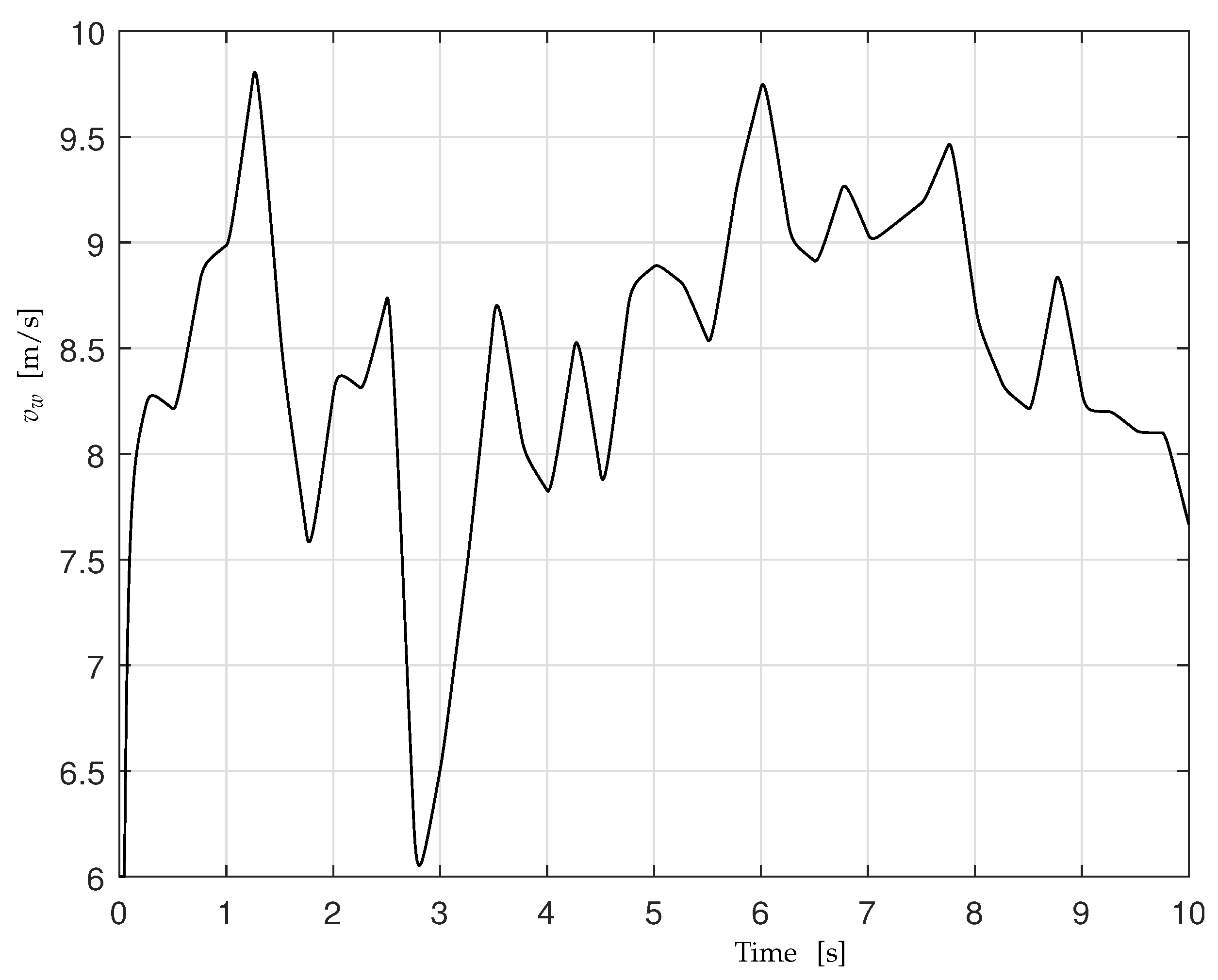
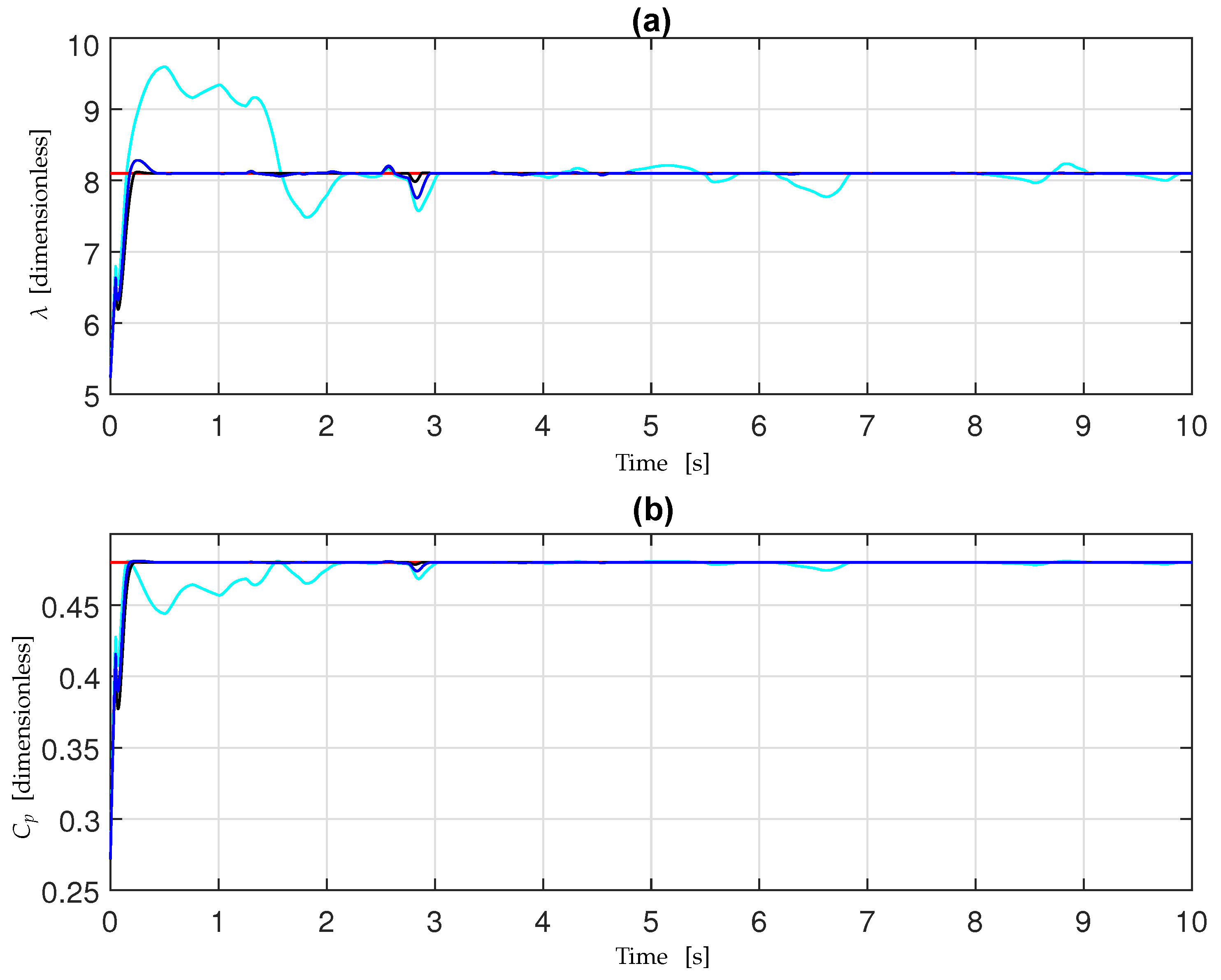
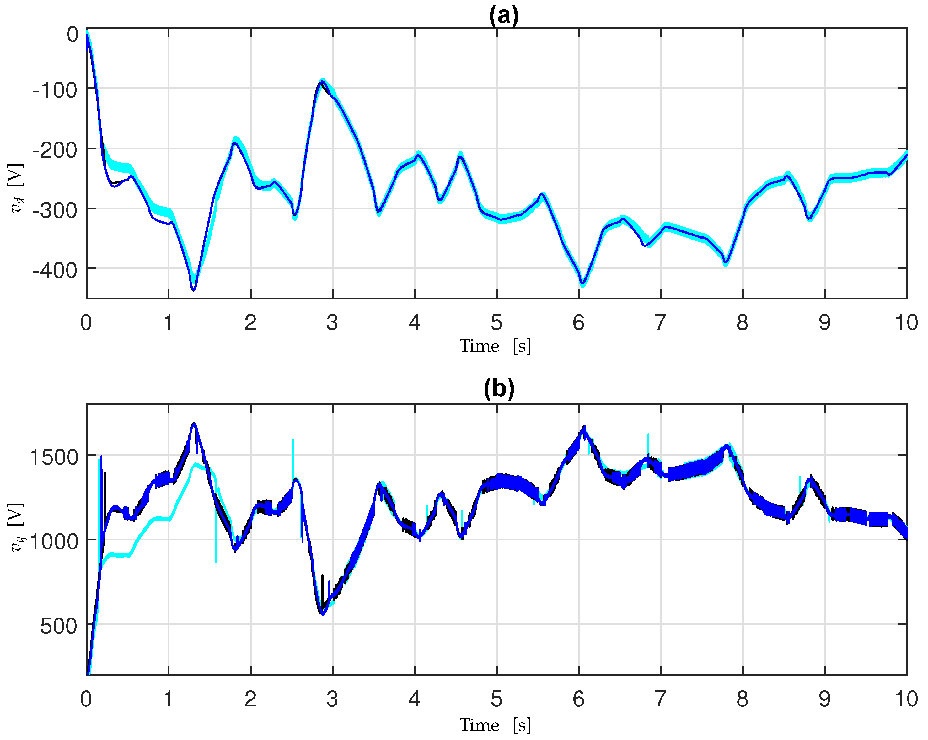
4. Simulation Results

The proposed dynamic controller (5) has been tested by numerical simulation using the mathematical model (1) of the PMSG-based WT. The simulations have been carried out in Simulink^®, which is a high-level language and interactive environment for numerical computation, visualization, and programming. It enables engineers to analyze data, develop algorithms, and create their own models and applications. Simulink^® is a toolbox included in the Matlab^® software (R2022a, The MathWorks Inc., Natick, MA, USA) for the modeling, simulation, and analysis of dynamic systems. It is a widely used tool in control engineering and signal processing for system simulation, signal processing for system simulation, and model-based design. Furthermore, the wind inflow used in the simulations consists of a data set of the turbulent wind that has been generated using the wind speed profile [51], as shown in Figure 3. Finally, the nominal values of the mechanical and electrical parameters of the considered WT are given in

Table 1. WT’s nominal parameter values.

$R^{\circ }$	Rotor radius	46.6 m
$R_s^{\circ }$	Winding resistance	0.821 $\mathsf{\Omega }$
$L^{\circ }$	Winding inductance	1.5731 $\times {10}^{-3}$ H
${\varphi }_m^{\circ }$	Flux linkage	5.8264 Wb
p	Pole number	26
$J^{\circ }$	Mechanical inertia	34.6 $\times {10}^3$ Kg m${}^2$
$f^{\circ }$	Coefficient of viscous friction	1.5 $\times {10}^{-3}$ Kg m${}^2$/s
${\rho }^{\circ }$	Normal air density	1.225 Kg/m${}^3$

, whilst, in

Table 2. WT’s actual parameter values.

$R=R^{\circ }$	$R_s=1.2R_s^{\circ }$	$L=0.95L^{\circ }$
${\varphi }_m=0.98{\varphi }_m^{\circ }$	$J=1.05J^{\circ }$	$f=0.8f^{\circ }$

, the actual parameter values are reported.

Some of the performances achieved in the simulations by the proposed controller (5), using the gains given in

Table 3. Controller gains.

${\gamma }_{1,1}=1380$	${\gamma }_{2,1}=1820$	${\gamma }_{3,1}=26$
${\gamma }_{1,2}=1320$	${\gamma }_{2,2}=1790$	${\gamma }_{3,2}=23$

and

Table 4. HOSM estimator gains.

${\alpha }_{1,1}=1200$	${\alpha }_{2,1}=5650$	${\alpha }_{3,1}=380$
${\alpha }_{1,2}=1180$	${\alpha }_{2,2}=5600$	${\alpha }_{3,2}=320$

, have been reported in Figure 4, Figure 5, Figure 6, Figure 7, Figure 8, Figure 9 and Figure 10. The considered initial conditions have been $i_{d,0}=0.5$ A, $i_{q,0}=18$ A, ${\omega }_0=10.47$ rad/s. The proposed robust nonlinear controller (5) has been compared with the same Controller (5) but without the estimation terms provided by the HOSM estimators. For further comparison, it has been compared also with the FOSM controller provided by [52]. It is crucial to note that the latter controller exhibits robustness in the face of system parameter variations. However, it is associated with the well-known chattering phenomenon, which is a notable drawback in such controllers. This particular drawback is clearly absent in the proposed controller. On the other hand, the proposed controller utilizes HOSM estimators, which confer robustness to the controller in the case of parameter variation with respect to the nominal values but, at the same time, avoid chattering phenomena (cf. [23] and reference therein).

The good performance achieved by the proposed controller in comparison with the other ones in terms of extracted energy is testified for by the simulation results. In fact, Figure 4a shows that the tip–speed ratio $\lambda$ is maintained close to its optimal value ${\lambda }_{max}^{\circ }$, and Figure 4b shows the $C_p$ coefficient, which is, most of the time, close to the optimal value $C_{p,max}^{\circ }$. On the other hand, Figure 5 shows that the proposed controller allows for extraction of the maximum wind power. Indeed, over the 10 s simulation interval, the proposed controller (5) enables the extraction of an additional 293.7783 W compared to the identical controller lacking HOSM estimators and a further 702.3711 W compared to the FOSM controller introduced in [52]. Furthermore, Figure 6 shows the behavior of the d-axis stator’s current $i_d$ and its reference $i_{d,\mathrm{ref}}=\phi \left(t\right)=0$; the q-axis stator current $i_q$ and its reference $i_{q,\mathrm{ref}}$; and the tracking error $e_{i_q}=i_q-i_{q,\mathrm{ref}}$. It is possible to observe that the proposed robust nonlinear controller exhibits improved behavior in comparison with the same controller without the HOSM estimation terms, as well as in comparison with the FOSM controller proposed in [52]. The behaviors of the angular velocity $\omega$ with respect to its reference ${\omega }_{\mathrm{ref}}$ and of the tracking error $e_{\omega }=\omega -{\omega }_{\mathrm{ref}}$ are shown in Figure 7. Once again, a better behavior of the proposed controller can be appreciated compared to the others. Figure 8 shows the stator voltages on the $d,q$-axis, i.e., $v_d$ and $v_q$. It can be observed that the proposed controller has less control effort than the other controllers considered in this analysis. The simulations demonstrate that the proposed robust nonlinear controller effectively achieves precise reference tracking. Given that the angular velocity reference was established using the MPPT technique, these performances contribute to maximizing the power extraction by the WT from the available wind resources. As already commented, the HOSM estimators, embedded in the proposed controller, provide robustness to the closed-loop system with respect to the perturbation terms. This can be appreciated in Figure 9, where the outputs of the robust differentiators embedded in the dynamic controller (5), i.e., ${\xi }_{1,1}$, ${\xi }_{2,1}$, ${\xi }_{3,1}$, are compared with the tracking errors $e_{i_d}$, $e_{i_q}$, $e_{\omega }$, respectively; furthermore, the errors ${\xi }_{1,1}-e_{i_d}$, ${\xi }_{2,1}-e_{i_q}$, ${\xi }_{3,1}-e_{\omega }$ are shown. Finally, the perturbations ${∆}_1$, ${∆}_2$, ${∆}_3$ and their estimations ${\xi }_{1,2}$, ${\xi }_{2,2}$, ${\xi }_{3,2}$, implemented in the proposed controller, are shown in Figure 10, including the estimation errors ${\xi }_{2,1}-{∆}_1$,${\xi }_{2,2}-{∆}_2$, ${\xi }_{3,2}-{∆}_3$. These results indicate that the HOSM estimators effectively estimate the perturbations, thereby ensuring accurate control performances with viable control actions.

To comprehensively assess the performance of the proposed controller, as well as the influence of the HOSM estimators on its effectiveness, performance indices have been computed in

Table 5. Performance indices for the tracking error $e_{i_d}=i_d-i_{d,\mathrm{ref}}$.

	MAE	MSE	IAE	ISE
Proposed controller (5)	$1.3\times {10}^{-3}$	$1.1000\times {10}^{-5}$	0.0132	$9.753\times {10}^{-5}$
Proposed controller (5)	$7.8\times {10}^{-3}$	$12.105\times {10}^{-5}$	0.0781	$120\times {10}^{-5}$
without the HOSM estimators
FOSM controller [52]	$4.6\times {10}^{-3}$	$4.529\times {10}^{-5}$	0.0458	$44.047\times {10}^{-5}$

,

Table 6. Performance indices for the tracking error $e_{i_q}=i_q-i_{q,\mathrm{ref}}$.

	MAE	MSE	IAE	ISE
Proposed controller (5)	0.7308	0.9520	7.3074	9.51
Proposed controller (5)	1.2428	4.7522	12.427	47.5119
without the HOSM estimators
FOSM controller [52]	7.8952	239.8277	78.9517	$2.3983\times {10}^3$

and

Table 7. Performance indices for tracking error $e_{\omega }=\omega -{\omega }_{\mathrm{ref}}$.

	MAE	MSE	IAE	ISE
Proposed controller (5)	0.0697	0.2099	0.6969	2.0978
Proposed controller (5)	0.0804	0.2441	0.80364	2.4396
without the HOSM estimators
FOSM controller [52]	0.6559	1.7382	6.5584	17.380

. These indices offer quantitative evaluations of the tracking performance, including the mean absolute error (MAE), the mean square error (MSE), the integral absolute error (IAE), and theiIntegral squared error (ISE). These metrics have also been computed for the same controller without the HOSM estimates and for the FOSM controller proposed in [52]. Once again, these indices confirm the superiority of the proposed approach in terms of performance.

5. Conclusions

In this work, a robust nonlinear dynamic controller has been designed for a WT with a PMSG. This controller ensures the maximization of the power extracted by the WT from the wind. To design the controller, a tracking problem was solved, ensuring the accurate tracking of an angular velocity reference for the WT blades. The wind velocity was assumed to be unavailable for direct measurement, and an estimator of the wind velocity was employed. Furthermore, a high-order sliding mode (HOSM) parameter estimator was utilized to compensate for the unknown perturbation terms, resulting in high-performance control of the WT. The simulations demonstrate the good performance of the controller. A comparison has been performed with the same controller but without the HOSM estimator terms, in terms of control performance and of the power extracted by the WT from the wind. Finally, the same comparison has been made with a classical FOSM controller. Future works will encompass the digital implementation of the proposed controller on a digital platform, along with the conduction of experimental tests through the utilization of hardware-in-the-loop techniques.

References

1. Chen, P.; Han, D. Effective wind speed estimation study of the wind turbine based on deep learning. Energy 2022, 247, 123491. [Google Scholar] [CrossRef]
2. Avendano-Valencia, L.D.; Abdallah, I.; Chatzi, E. Virtual fatigue diagnostics of wake-affected wind turbine via Gaussian process regression. Renew. Energy 2021, 170, 539–561. [Google Scholar] [CrossRef]
3. Mohammadi, E.; Rasoulinezhad, R.; Moschopoulos, G. Using a Supercapacitor to Mitigate Battery Microcycles Due to Wind Shear and Tower Shadow Effects in Wind-Diesel Microgrids. IEEE Trans. Smart Grid 2020, 11, 3677–3689. [Google Scholar] [CrossRef]
4. Benmahdjoub, M.A.; Mezouar, A.; Ibrahim, M.; Boumediene, L.; Saidi, Y.; Atallah, M. Accurate Estimation of Effective Wind Speed for Wind Turbine Control Using Linear and Nonlinear Kalman Filters. Arab. J. Sci. Eng. 2023, 48, 6765–6781. [Google Scholar] [CrossRef]
5. Amato, F.; Guignard, F.; Walch, A.; Mohajeri, N.; Scartezzini, J.L.; Kanevski, M. Spatio-temporal estimation of wind speed and wind power using extreme learning machines: Predictions, uncertainty and technical potential. Stoch. Environ. Res. Risk Assess. 2022, 36, 2049–2069. [Google Scholar] [CrossRef] [PubMed]
6. Bhowmik, S.; Spee, R.; Enslin, J.H.R. Performance Optimization for Doubly Fed Wind Power Generation Systems. IEEE Trans. Ind. Appl. 1999, 35, 949–958. [Google Scholar] [CrossRef]
7. Utkin, V.I. Sliding Modes in Control and Optimization; Springer: Berlin/Heidelberg, Germany, 1992. [Google Scholar]
8. Pourebrahim, R.; Shotorbani, A.M.; Márquez, F.P.G.; Tohidi, S.; Mohammadi-Ivatloo, B. Robust Control of a PMSG-Based Wind Turbine Generator Using Lyapunov Function. Energies 2021, 14, 1712. [Google Scholar] [CrossRef]
9. Mousavi, Y.; Bevan, G.; Kucukdemiral, I.B.; Fekih, A. Sliding mode control of wind energy conversion systems: Trends and applications. Renew. Sustain. Energy Rev. 2022, 167, 112734. [Google Scholar] [CrossRef]
10. Rajendran, S.; Jena, D. Backstepping Sliding Mode Control of a Variable Speed Wind Turbine for Power Optimization. J. Mod. Power Syst. Clean Energy 2015, 3, 402–410. [Google Scholar] [CrossRef]
11. Corradini, M.L.; Ippoliti, G.; Orlando, G. A Sliding Mode Pitch Controller for Wind Turbines Operating in High Wind Speeds Region. In Proceedings of the International Conference on Control, Decision and Information Technologies, Barcelona, Spain, 5–7 April 2017; pp. 1–6. [Google Scholar] [CrossRef]
12. Gajewski, P.; Pieńkowski, K. Analysis of Sliding Mode Control of Variable Speed Wind Turbine System with PMSG. In Proceedings of the International Symposium on Electrical Machines (SME), Naleczow, Poland, 18–21 June 2017; pp. 1–6. [Google Scholar] [CrossRef]
13. Ardjal, A.; Mansouri, R.; Bettayeb, M. Fractional sliding mode control of wind turbine for maximum power point tracking. Trans. Inst. Meas. Control 2018, 41, 447–457. [Google Scholar] [CrossRef]
14. Yang, B.; Yu, T.; Shu, H.; Dong, J.; Jiang, L. Robust sliding—Mode control of wind energy conversion systems for optimal power extraction via nonlinear perturbation observers. Appl. Energy 2018, 210, 711–723. [Google Scholar] [CrossRef]
15. Mohammad, J.M.; Afef, F. A Sliding Mode Approach to Enhance the Power Quality of Wind Turbines Under Unbalanced Voltage Conditions. IEEE/CAA J. Autom. Sin. 2019, 2, 566–574. [Google Scholar] [CrossRef]
16. Fridman, L.; Moreno, J.; Iriarte, R. Sliding Modes after the first Decade of the 21st Century: State of the Art. Lect. Notes Control Inf. Sci. 2011, 412, 113–149. [Google Scholar]
17. Emelyanov, S.V.; Korovin, S.K.; Levantovsky, L.V. Higher Order Sliding Regimes in the Binary Control Systems. Sov. Phys. 1986, 31, 291–293. [Google Scholar]
18. Edwards, C.; Spurgeon, S.K. Sliding Mode Control: Theory and Application; Taylor and Francis Ltd.: London, UK, 1999. [Google Scholar]
19. Bartolini, G.; Pisano, A.; Usai, E. First and Second Derivative Estimation by Sliding Mode Technique. J. Signal Process. 2000, 4, 167–176. [Google Scholar]
20. Fridman, L.; Levant, A. Higher Order Sliding Modes, Sliding Mode Control in Engineering; Marcel Dekker: New York, NY, USA, 2002; pp. 53–101. [Google Scholar]
21. Floquet, T.; Barbot, J.P. Super Twisting Algorithm based Step–by–Step Sliding Mode Observers for Nonlinear Systems with Unknown Inputs. Int. J. Syst. Sci. 2007, 10, 803–815. [Google Scholar] [CrossRef]
22. Levant, A. Higher–Order Sliding Modes, Differentiation and Output Feedback Control. Int. J. Control 2003, 76, 924–941. [Google Scholar] [CrossRef]
23. Fridman, L.; Shtessel, Y.; Edwards, C.; Yan, X.G. Higher–Order Sliding–Mode Observer for State Estimation and Input Reconstruction in Nonlinear Systems. Int. J. Robust Nonlinear Control 2008, 18, 399–413. [Google Scholar] [CrossRef]
24. Levant, A. Homogeneity Approach to High–Order Sliding Mode Design. Automatica 2005, 41, 823–830. [Google Scholar] [CrossRef]
25. Basin, M.V.; Yu, P.; Shtessel, Y.B. Hypersonic Missile Adaptive Sliding Mode Control Using Finite-and Fixed-Time Observers. IEEE Trans. Ind. Electron. 2018, 65, 930–941. [Google Scholar] [CrossRef]
26. Deng, H.; Li, Q.; Chen, W.; Zhang, G. High–Order Sliding Mode Observer Based OER Control for PEM Fuel Cell Air–Feed System. IEEE Trans. Energy Convers. 2018, 33, 232–244. [Google Scholar] [CrossRef]
27. Kommuri, S.K.; Lee, S.B.; Veluvolu, K.C. Robust Sensors–Fault–Tolerance With Sliding Mode Estimation and Control for PMSM Drives. IEEE/ASME Trans. Mechatronics 2018, 23, 17–28. [Google Scholar] [CrossRef]
28. Pan, Y.; Yang, C.; Pan, L.; Yu, H. Integral Sliding Mode Control: Performance, Modification, and Improvement. IEEE Trans. Ind. Inform. 2018, 14, 3087–3096. [Google Scholar] [CrossRef]
29. Panathula, C.B.; Rosales, A.; Shtessel, Y.B.; Fridman, L.M. Closing Gaps for Aircraft Attitude Higher Order Sliding Mode Control Certification via Practical Stability Margins Identification. IEEE Trans. Control. Syst. Technol. 2018, 26, 2020–2034. [Google Scholar] [CrossRef]
30. Liu, J.; Gao, Y.; Su, X.; Wack, M.; Wu, L. Disturbance Observer Based Control for Air Management of PEM Fuel Cell Systems via Sliding Mode Technique. IEEE Trans. Control Syst. Technol. 2018, 27, 1129–1138. [Google Scholar] [CrossRef]
31. Gao, Y.; Liu, J.; Sun, G.; Liu, M.; Wu, L. Fault Deviation Estimation and Integral Sliding Mode Control Design for Lipschitz Nonlinear Systems. Syst. Control Lett. 2019, 123, 8–15. [Google Scholar] [CrossRef]
32. Van, M. An Enhanced Tracking Control of Marine Surface Vessels Based on Adaptive Integral Sliding Mode Control and Disturbance Observer. ISA Trans. 2019, in press. [CrossRef]
33. Karim, B.; Sami, B.S.; Adnane, C. Higher Order Sliding mode control For PMSG in Wind power Conversion System. In Proceedings of the 2016 4th International Conference on Control Engineering & Information Technology (CEIT), Hammamet, Tunisia, 16–18 December 2016; pp. 1–6. [Google Scholar]
34. Valenciaga, F.; Puleston, P.F. High-Order Sliding Control for a Wind Energy Conversion System Based on a Permanent Magnet Synchronous Generator. IEEE Trans. Energy Convers. 2008, 23, 860–867. [Google Scholar] [CrossRef]
35. Barambones, O.; Gonzalez de Durana, J.M. Adaptive sliding mode control strategy for a wind turbine systems using a HOSM wind torque observer. In Proceedings of the IEEE International Energy Conference (ENERGYCON), Leuven, Belgium, 4–8 April 2016; pp. 1–610. [Google Scholar] [CrossRef]
36. Barambones, O.; González de Durana, J.M. Second Order Sliding Mode Controller and Observer for a Wind Turbine System. In Proceedings of the 2017 IEEE International Conference on Environment and Electrical Engineering and 2017 IEEE Industrial and Commercial Power Systems Europe (EEEIC/I CPS Europe), Milan, Italy, 6–9 June 2017; pp. 1–6. [Google Scholar]
37. Merabet, A. Adaptive Sliding Mode Speed Control for Wind Energy Experimental System. Energies 2018, 11, 2238. [Google Scholar] [CrossRef]
38. Zine Laabidine, N.; Bossoufi, B.; El Kafazi, I.; El Bekkali, C.; El Ouanjli, N. Robust Adaptive Super Twisting Algorithm Sliding Mode Control of a Wind System Based on the PMSG Generator. Sustainability 2023, 15, 10792. [Google Scholar] [CrossRef]
39. Matraji, I.; Al-Durra, A.; Errouissi, R. Design and experimental validation of enhanced adaptive second-order SMC for PMSG-based wind energy conversion system. Int. J. Electr. Power Energy Syst. 2018, 103, 21–30. [Google Scholar] [CrossRef]
40. Zhang, C.; Plestan, F. Individual/collective blade pitch control of floating wind turbine based on adaptive second order sliding mode. Ocean Eng. 2021, 228, 108897. [Google Scholar] [CrossRef]
41. Fdaili, M.; Essadki, A.; Kharchouf, I.; Nasser, T. An overall modeling of wind turbine systems based on DFIG using conventional sliding mode and second-order sliding mode controllers. In Proceedings of the 2019 International Conference on Wireless Technologies, Embedded and Intelligent Systems (WITS), Fez, Morocco, 3–4 April 2019; pp. 1–6. [Google Scholar] [CrossRef]
42. Zargham, F.; Mazinan, A.H. Super-twisting sliding mode control approach with its application to wind turbine systems. Energy Syst. 2019, 10, 211–229. [Google Scholar] [CrossRef]
43. Bianchi, F.D.; Battista, H.N.D.; Mantz, R.J. Wind Turbine Control Systems: Principles, Modelling and Gain Scheduling Design; Springer: Berlin/Heidelberg, Germany, 2007. [Google Scholar]
44. Siegfried, H. Grid Integration of Wind Energy Conversion Systems; Wiley: New York, NY, USA, 1998. [Google Scholar]
45. Zaragoza, J.; Pou, J.; Arias, A.; Spiteri, C.; Robles, E.; Ceballos, S. Study and Experimental Verification of Control Tuning Strategies in a Variable Speed Wind Energy Conversion System. Renew. Energy 2011, 36, 1421–1430. [Google Scholar] [CrossRef]
46. Moreno, J.A.; Osorio, M. A Lyapunov Approach to Second–Order Sliding Mode Controllers and Observers. In Proceedings of the 2008 47th IEEE Conference on Decision and Control, Cancun, Mexico, 9–11 December 2008; pp. 2856–2861. [Google Scholar]
47. Moreno, J.A. Lyapunov Approach for Analysis and Design of Second Order Sliding Mode Algorithms. In Sliding Modes after the First Decade of the 21st Century: State of the Art; Lecture Notes in Control and Information Sciences; Thoma, M., Allgöwer, F., Morari, M., Eds.; Springer: Berlin/Heidelberg Germany, 2011. [Google Scholar]
48. Khalil, H.K. Nonlinear Systems, 3rd ed.; Prentice–Hall: Englewood Cliffs, NJ, USA, 2002. [Google Scholar]
49. Clarke, F.H.; Ledyaev, Y.; Stern, R.J.; Wolenski, P.R. Nonsmooth Analysis and Control Theory; Springer: New York, NY, USA, 1998. [Google Scholar]
50. Cortés, J. Discontinuous Dynamical Systems: A Tutorial on Solutions, Nonsmooth Analysis, and Stability. IEEE Control Syst. Mag. 2008, 28, 36–73. [Google Scholar]
51. Introduction to Wind Speed Monitoring for Wind Turbines. 2021. Available online: https://www.windlogger.com/blogs/news/5116392-introduction-to-wind-speed-monitoring-for-wind-turbines (accessed on 30 July 2023).
52. Corradini, M.L.; Ippoliti, G.; Orlando, G. Robust Control of Variable-Speed Wind Turbines Based on an Aerodynamic Torque Observer. IEEE Trans. Control Syst. Technol. 2013, 21, 1199–1206. [Google Scholar] [CrossRef]
Figure 1. Scheme of a WT with a PMSG.
Energies 16 06649 g001
Figure 2. Scheme of the closed-loop system of the WT equipped with a PMSG and controlled by controller (5).
Energies 16 06649 g002
Figure 3. Wind velocity profile v w .
Energies 16 06649 g003
Figure 4. (a) Tip–speed ratio λ : proposed method (5) (black), proposed method (5) without the HOSM estimators (blue), FOSM (cyan), and λ max (red); (b) power coefficient C p : proposed method (5) (black), proposed method (5) without the HOSM estimators (blue), FOSM (cyan), and C p , max (red).
Energies 16 06649 g004
Figure 5. Power extracted by the WT: proposed method (5) (black), proposed method (5) without the HOSM estimators (magenta), FOSM (cyan).
Energies 16 06649 g005
Figure 6. (a) Stator current i d : Proposed method (5) (black), proposed method (5) without the HOSM estimators (blue), FOSM (cyan), and reference i d , ref = 0 ; (b) stator current i q : proposed method (5) (black), proposed method (5) without the HOSM estimators (blue), FOSM (cyan), and reference i q , ref (red); (c) tracking error e i d : proposed method (5) (black), proposed method (5) without the HOSM estimators (blue), and FOSM (cyan); (d) tracking error e i q : proposed method (5) (black), proposed method (5) without the HOSM estimators (blue), and FOSM (cyan).
Energies 16 06649 g006
Figure 7. (a) Angular velocity ω : proposed method (5) (black), proposed method (5) without the HOSM estimators (blue), FOSM (cyan), and reference ω ref (red); (b) tracking error e ω : proposed method (5) (black), proposed method (5) without the HOSM estimators (blue), and FOSM (cyan).
Energies 16 06649 g007
Figure 8. (a) Stator voltage v d : proposed method (5) (black), proposed method (5) without the HOSM estimators (blue), and FOSM (cyan); (b) stator voltage v q : proposed method (5) (black), proposed method (5) without the HOSM estimators (blue), and FOSM (cyan).
Energies 16 06649 g008
Figure 9. Error estimations: (a) ξ 1 , 1 (red) and tracking error e i d (black); (b) ξ 2 , 1 (red) and tracking error e i q (black); (c) ξ 3 , 1 (red) and tracking error e ω (black); (d) ξ 1 , 1 e i d ; (e) ξ 2 , 1 e i q ; (f) ξ 3 , 1 e ω .
Energies 16 06649 g009
Figure 10. Velocity error estimations: (a) ξ 1 , 2 (red) and 1 (black); (b) ξ 2 , 2 (red) and 2 (black); (c) ξ 3 , 1 (red) and 3 (black); (d) ξ 2 , 1 1 ; (e) ξ 2 , 2 2 ; (f) ξ 3 , 2 3 .
Energies 16 06649 g010