Abstract
The subject of electric vehicles (EVs) is constantly relevant from the perspective of climate change and sustainability. Multi-Criteria Decision Analysis (MCDA) methods can be successfully used to evaluate models of such vehicles. In many cases, the MCDA methods are modified to account for uncertainty in the data. There are many ways to express uncertainty, including more advanced ones, such as fuzzy sets, for example, but expressing attributes in terms of interval numbers remains a popular method because it is an easy-to-implement and easy-to-understand technique. This study focuses on interval extensions of the TOPSIS (Technique for Order Preference by Similarity to Ideal Solution) method. It aims to compare the most popular extension proposed by Jahanshahloo and the proposed new modification, which returns the result in an interval form. Certain inconsistencies of the Jahanshahloo extension are discussed, and it is explained how the new extension avoids them. Both extensions are applied to an EV evaluation problem taken from the literature as an example for sustainable assessment. The results are then analyzed, and the question of whether the input data of the interval should receive an evaluation in the form of interval results is addressed.
1. Introduction
MCDA (Multi-Criteria Decision Analysis) methods are a useful and expanding tool to assist in the decision-making process in various disciplines [1], such as health care [2], environmental sciences [3], energy and environmental modeling [4], natural resource management [5], or finances [6]. In MCDA problems, a given set of alternatives is present and subject to evaluation. These alternatives are described by multiple criteria that often conflict with each other [7]. The requirement for sustainable solutions, particularly in the realm of electric vehicles, is increasing, making it necessary to have reliable and adjustable decision-making tools such as TOPSIS with interval numbers.
An example of such a problem is the evaluation of electric vehicles (EVs). The topic of EVs is important and relevant as it relates to environmental protection and sustainability [8,9,10]. EVs are mentioned as a technology that offers the opportunity to reduce CO2 emissions and noise [11]. In the literature, there are examples of applications of MCDA methods to EV evaluation and selection problems [10,12,13]. Although studies also occur for other types of vehicles, such as electric cargo bikes [14] and aircraft [15], electric cars remain the most popular subject. Frequently mentioned metrics when evaluating EVs are driving range, price, and charging speed [9,16,17]. Battery-related concerns also arise, which is an important factor not only from the consumer’s point of view [18], but also an influential variable from a development point of view [19,20]. Electric vehicles can also be examined from the angle of energy consumption. However, research suggests that this characteristic is influenced by various factors and there are ways to optimize it [21,22,23]. Some of the EV features can easily be used as criteria for the application of MCDA methods [24]. Quantitative criteria often discussed in relation to EVs, in addition to those mentioned, include maximum power [17,25], cargo volume [26], top speed [13,17,27], and acceleration [17,28]. There are also qualitative attributes, such as reliability [9], safety [29], comfort [20], or prestige [29]. The use of these, however, might bring uncertainty into the problem as they often cannot be straightforwardly expressed in numerical units.
One of the most popular MCDA methods is TOPSIS (Technique for Order Preference by Similarity to Ideal Solution) proposed in 1981 by Hwang and Yoon [30]. At the basis of the TOPSIS method is the identification of what are called ideal solutions; namely, a positive ideal solution (PIS) and a negative ideal solution (NIS). The alternatives are evaluated based on their distance from the aforementioned ideal solutions. Essentially, they obtain a better score the shorter their distance from PIS and the greater their distance from NIS. The TOPSIS method has many advantages that contribute to its popularity. Among the most apparent are its simplicity and efficiency [31], ability to be adapted to deal with both quantitative and qualitative data [32], and the fact that no advanced tools or knowledge are required to implement it [33].
The popularity of the TOPSIS method is reflected in its large presence in the literature. Behzadian et al. [34] created a well-known literature review in which they described and categorized 266 papers from 2000 to 2012 that employ the TOPSIS method. TOPSIS is also commonly used in the present day [35]. Areas of its application include sustainability [36,37,38,39], finances [40,41,42], energy planning and management [43,44,45], and transportation [46,47,48]. Among the applications listed, not only the original TOPSIS method is used, but also combinations with other methodologies and different extensions adapted to the addressed issue.
An important advantage of the TOPSIS method is its susceptibility to creating extensions. Many extensions of the TOPSIS method are based on fuzzy numbers [49] or interval numbers [50]. However, new types of uncertainty data, such as basic uncertain information and others, are still being developed [51]. Such approaches are associated with uncertainty in the data, as in some problems, the attribute values of alternatives to criteria cannot be unambiguously determined. This is a common concern in MCDA methods in general [52,53]. Many other MCDA methods have also been adapted to deal with uncertain data; for example, PROMETHEE (Preference Ranking Organization Method of Enrichment Evaluation) [54], VIKOR (VlseKriterijumska Optimizacija I Kompromisno Resenje) [55], and COMET (Characteristic Objects METhod) [56]. Moreover, Jin et al. introduce in [57] two novel concepts in handling uncertainty: interval extensions of cognitive interval information and cognitive uncertain information, which replace real-numbered values with intervals. These extensions exhibit enhanced algorithmic versatility and applicability, particularly in group decision-making scenarios. This provides the opportunity to employ the interval-valued operator as a means of combining interval-valued functions [58].
An overview of the applications of fuzzy TOPSIS variants is provided by Palczewski and Sałabun [59]. This study focuses on extensions of the TOPSIS method that operate on interval numbers. There are many extensions of this kind that approach the use of intervals in different ways [60,61,62,63]. A popular extension is the interval TOPSIS proposed by Jahanshahloo [60], in which the PIS and NIS, as well as the final evaluation of alternatives, are crisp numbers. Another existing extension is the direct interval extension by Dymova [63]. Here, PIS and NIS are expressed in interval form, but the evaluation of alternatives is a crisp number. It is noticeable that in such cases some nuances are disregarded. Since the alternatives are given in the form of interval values, it seems logical that a crisp result could result in a loss of accuracy.
This paper aims to investigate a comprehensive analysis of the comparative performance between two innovative extensions of the TOPSIS method, which are tailored to operate specifically within the domain of intervals. The conventional interval TOPSIS approach, as proposed by Jahanshahloo, derives preference values for alternatives as precise real numbers [60]. On the contrary, the novel methodology introduced in this study generates preference values as intervals [64]. Through this investigation, our primary objective is to evaluate the robustness and consistency of the results produced by these two distinct approaches and, furthermore, to elucidate how such a fundamental difference in methodology can potentially impact the decision-making process. To enable a meaningful comparison between these two methods, we propose a simple approach to represent the intervals obtained in our extension as crisp values (left bound, right bound, or midpoint). It is important to highlight that in our extension, each preference is explicitly expressed as an interval with defined minimum and maximum possible values. The use of midpoints is primarily for the purpose of comparison with the Jahanshahloo approach, where preference values are presented as single, noninterval numbers. In the Jahanshahloo approach, the use of single crisp values may impose limitations in capturing the inherent variability and uncertainty inherent in the decision-making process.
The rest of the paper is structured as follows. Section 2 provides a detailed description of how the TOPSIS method and its discussed interval extensions operate. Section 3 contains a numerical example involving data on EVs. Section 4 contains the analysis of the results and discussion. Finally, Section 5 provides a summary and direction for further research.
2. Materials and Methods
This section presents the algorithms of TOPSIS and its considered extensions. Next, the coefficients used to determine the similarity of the rankings are presented. Finally, the method for obtaining interval numbers used in this study is explained.
2.1. The TOPSIS Method
In the classic TOPSIS method, the problem is given in the form of a decision matrix M with m alternatives and n criteria, as well as a vector of weights [65].
In the decision matrix, is the attribute of the j-th alternative () to the i-th criterion (). The vector is a vector of weights associated with each criterion—one weight is assigned to every criterion .
- Step 1.
- Normalize the decision matrix, where is the normalized attribute of the alternative against the criterion :
- Step 2.
- Calculate the weighted normalized decision matrix, where is the weighted normalized attribute of the alternative against the criterion :
- Step 3.
- Determine the positive ideal solution PIS () and the negative ideal solution NIS ():where I stands for profit-type criteria, and J stands for cost-type criteria.
- Step 4.
- Calculate the separation (as Euclidean distance) of each alternative from the positive ideal solution and from the negative ideal solution , respectively:
- Step 5.
- Determine the relative closeness of each alternative to the positive ideal solution :
- Step 6.
- Rank each alternative by the values of their obtained relative closeness . The higher the relative closeness , the better the position of alternative in the final ranking.
2.2. The Interval TOPSIS Method
In 2006, Jahanshahloo proposed an extension to the TOPSIS method that operates on interval numbers [60]. It provides a way to incorporate uncertain data into the decision-making process. In this approach, the algorithm is similar to the classic approach, but some operations have been adapted for the purpose of applying interval numbers. The problem is given in a similar form:
In the decision matrix, instead of crisp values, intervals [] are given. The value stands for the lower limit of the interval, whereas stands for the upper limit of the interval. To distinguish between the approaches, some of the symbols concerning the interval TOPSIS method feature a bar (e.g., as opposed to ).
In the interval TOPSIS method proposed by Jahanshahloo, the procedure is as follows.
- Step 1.
- Normalize the decision matrix, where i are, respectively, the lower and upper limit of the normalized interval attribute of the alternative to the criterion :
- Step 2.
- Calculate the weighted normalized decision matrix, where and are, respectively, the lower and upper limit of the weighted normalized interval attribute of the alternative to the criterion :
- Step 3.
- Determine the positive ideal solution PIS () and the negative ideal solution NIS ():where I stands for profit-type criteria, whereas J stands for cost-type criteria.
- Step 4.
- Calculate the separation of each alternative from the positive ideal solution and from the negative ideal solution , respectively:
- Step 5.
- Determine the relative closeness of each alternative to the positive ideal solution :
- Step 6.
- Rank each alternative as in the classical approach.
2.3. The New Approach
A significant difference between the interval TOPSIS and the new approach is the way the score is evaluated since in the new approach, the assessment of alternatives is given as an interval [64].
In the new approach, the first steps (1–3) are identical to those in the interval TOPSIS method. The decision matrix and the vector of weights are given in the same format. The positive and negative ideal solutions also remain the same. However, the method of determining the evaluation of each alternative is different. For each alternative (), the following steps are required:
- Step 4.1.
- Generate an auxiliary decision matrix , for which the classical TOPSIS method can be used. The individual alternatives are expressed as follows:where stands for the j-th of the m considered alternatives. Then, the generation of the auxiliary decision matrix for this alternative involves determining the Cartesian product of the lower and upper limits of the value of each criterion:The auxiliary decision matrix is then expressed as:where () is the j-th of the auxiliary alternatives.
- Step 4.2.
- Apply the classic TOPSIS method to the generated auxiliary decision matrix. Substitute the and determined in step 3 for PIS and NIS. Then calculate:
- Step 4.3.
- The result for alternative is an interval:
2.4. Correlation Coefficients
Correlation coefficients and similarity coefficients are used to provide a numerical expression of the similarity of two rankings. In this study, two coefficients described below were chosen to evaluate the rankings obtained from extensions of the TOPSIS method.
2.4.1. Weighted Spearman’s Rank Correlation Coefficient
In this approach, it is not only the occurrence of differences that affects the result, but also at which ranking position they occur. Differences in the top ranking positions are more significant than those in the bottom ranking positions [65,66]. This coefficient is defined as (19):
where N is the size sample, are the rank values of the first ranking, and are the rank values of the second ranking.
2.4.2. Rank Similarity Coefficient
This coefficient is asymmetric, with the first ranking being the reference ranking. The score is closely related to the ranking positions on which differences occur, with the top ranking positions being the most significant [65,66]. The coefficient is defined as (20):
where N is the size sample, are the rank values of the first ranking, and are the rank values of the second ranking.
2.5. Extending Crisp Numbers to Interval Numbers
In order to compare the performance of the extensions in question, it is necessary to provide data in interval form. In this paper, we propose the following method of extending crisp data to interval form (21):
where is an arbitrarily selected factor.
3. Study Case
The data in the example come from Dviwedi and Sharma [67], in which a comparison of 15 models of EVs is conducted. The authors take into consideration the following criteria:
- —total power, expressed in horsepower (hp);
- —electric range, expressed in kilometers (km);
- —battery capacity, expressed in kilowatt-hours (kWh);
- —top speed, expressed in kilometers per hour (km/h);
- —cargo volume, expressed in liters (l);
- —acceleration as the acceleration time from 0 to 100 km/h, expressed in seconds (s);
- —base price, expressed in British pound sterling (£);
- —fast charge time as the time of charging from to , expressed in minutes (min);
- —full charge time, expressed in hours (h);
- —unladen weight, expressed in kilograms (kg).
The data in the original paper are crisp data. For the purposes of this paper, they have been converted to interval data using Formula (21) with . This means that from each value an interval is derived with the lower limit reduced and the upper limit increased by of that value.
The original data can be found in Table 1. In addition to the attribute values for each criterion, the names of the EV models being evaluated are also included. The vector of weights is taken from the original paper without changes.

Table 1.
The crisp decision matrix.
The derived interval decision matrix can be found in Table 2. For criterion , the alternatives take values in the range , with an average of . For criterion , the range of values is and the mean is , for criterion there is a range of values of and a mean of , the range of values for criterion is and the mean is , and criterion has a range of values of and a mean of . The lowest mean value occurs for criterion ; it is with a range of values . Meanwhile, the highest average value occurs for criterion ; it is 83,334.67 whereas the range of values is [38,380.5, 153,208]. For the other criteria, the values are as follows: range and mean for , range and mean for , and range and mean for . Thus, it can be seen that the values within the criteria vary, and this indicates the need for normalization.
Table 2.
The interval decision matrix.
The normalized interval decision matrix can be found in Table 3. All values are scaled to interval . The results of the next stage of the calculation, which is weighting, can be found in Table 4. The ideal solutions identified are in Table 5. At this point, the common part of the calculations for interval TOPSIS and the new approach ends.
Table 3.
The normalized interval decision matrix.
Table 4.
The weighted normalized interval decision matrix.
Table 5.
Positive and negative ideal solutions.
The results obtained by applying the interval TOPSIS method are shown in Table 6. The best three alternatives suggested by this extension are (Tesla Model S Plaid), (Lucid Air Touring), and (Porsche Taycan Turbo) with relative closeness of , , and , respectively. In comparison, (Mercedes EQV 300) with relative closeness of was identified to be the least attractive alternative.
Table 6.
Results obtained by the interval TOPSIS method.
The results obtained from the application of the new approach can be found in Table 7. Since, with 10 criteria, the auxiliary decision matrices mentioned in Section 2.3 have rows, they are not presented here.
Table 7.
Results obtained by the new interval TOPSIS method.
For readability, the following designations of the final rankings are used in the remainder of the paper:
- —ranking obtained from interval TOPSIS;
- —ranking obtained from only the lower limits of the intervals resulting from the new approach;
- —ranking obtained from the mean of the interval limits resulting from the new approach;
- —ranking obtained from only the upper limits of the intervals resulting from the new approach.
Not all of the aforementioned rankings are consistent with each other. Most of the alternatives (–, –) are ranked the same in each case. This is particularly important regarding alternative , which holds the most significant first position in the ranking. However, there are differences for the remaining alternatives. Figure 1 provides a visual summary of all the rankings in question in the form of a bar chart.
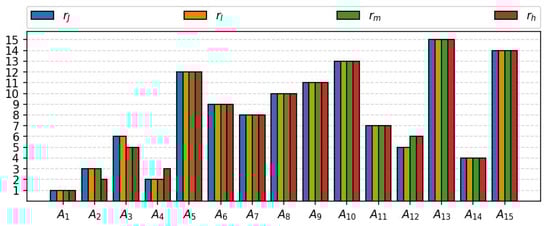
Figure 1.
A summary of the rankings , , , and in the form of a bar chart.
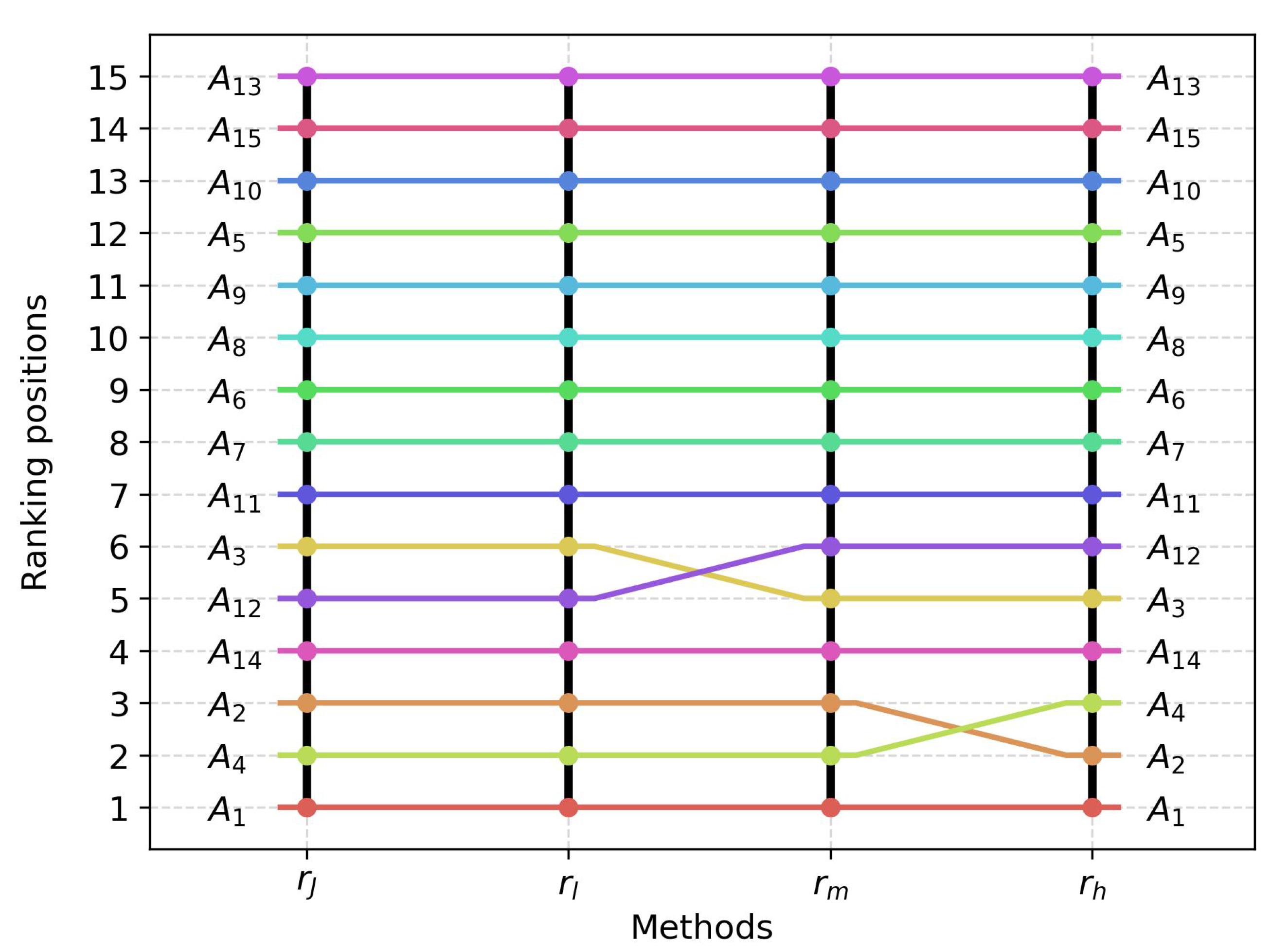
Figure 2 shows the differences between the ranking obtained from the interval TOPSIS and the individual rankings obtained from the new approach. The rankings of and appear first. In this case, both rankings turned out to be identical.
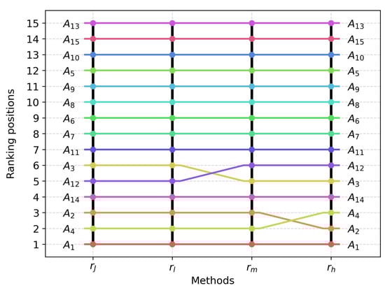
Figure 2.
Ranking flows featuring rankings , , , and .
The two rankings and agree on most positions. Only the alternatives and are interchanged with each other in these rankings. The interchange occurs in the 5th and 6th positions in the ranking, so the difference is not as significant as it would be if there were differences in the upper ranking positions.
The most differences occur between the rankings of and . They are also the most significant. In addition to the same interchange in ranking positions 5 and 6 as in comparison of and , there is also an interchange in positions 2 and 3 (alternatives and ). These are among the top-ranked positions, so they play a greater role in, for example, calculating selected correlation coefficients.
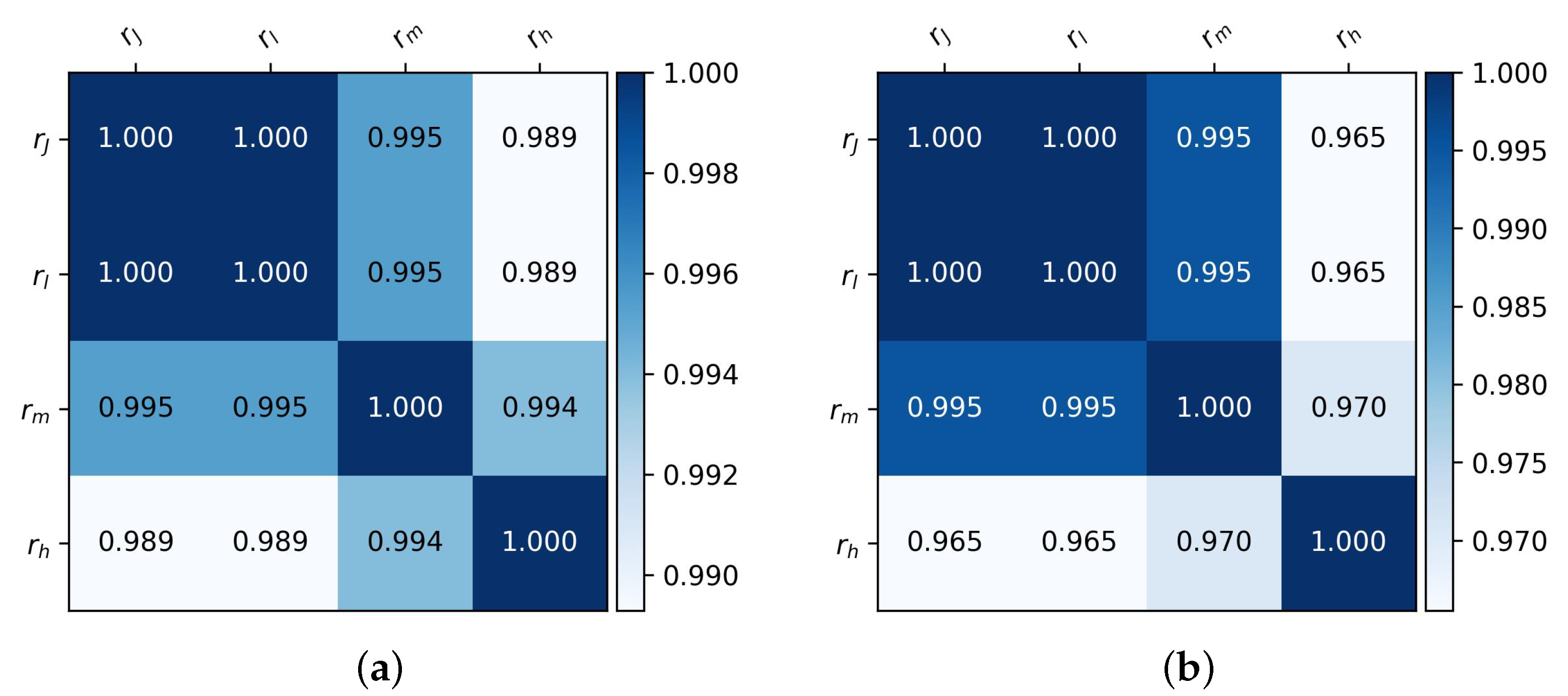
The calculated correlation coefficients between the rankings in the form of a correlation matrix can be found in Figure 3. As could be deduced from previous visualizations, the rankings and are the least similar to each other, scoring for the coefficient and for the coefficient. Even though this is the lowest of the results obtained, it still indicates that the two rankings are similar. Better results ( for both and ) are achieved by the and rankings, as differences in them occur less frequently and further down the ranking.

Figure 3.
Correlation matrices. (a) Weighted Spearman’s Rank Correlation Coefficient. (b) Rank similarity coefficient.
It is worth noting the similarity between the rankings of and . In Table 7 and Figure 2, one can see that they differ at positions 2 and 3. With this insight, it is possible to observe that it is indeed not only the occurrence of differences in rankings itself that matters, but also the position at which the differences occur. The results of for and for are worse than for the rankings of and , where there was also only one interchange, but at positions 5 and 6.
The rankings and are identical, so the value of both coefficients and for them equals 1.
4. Discussion
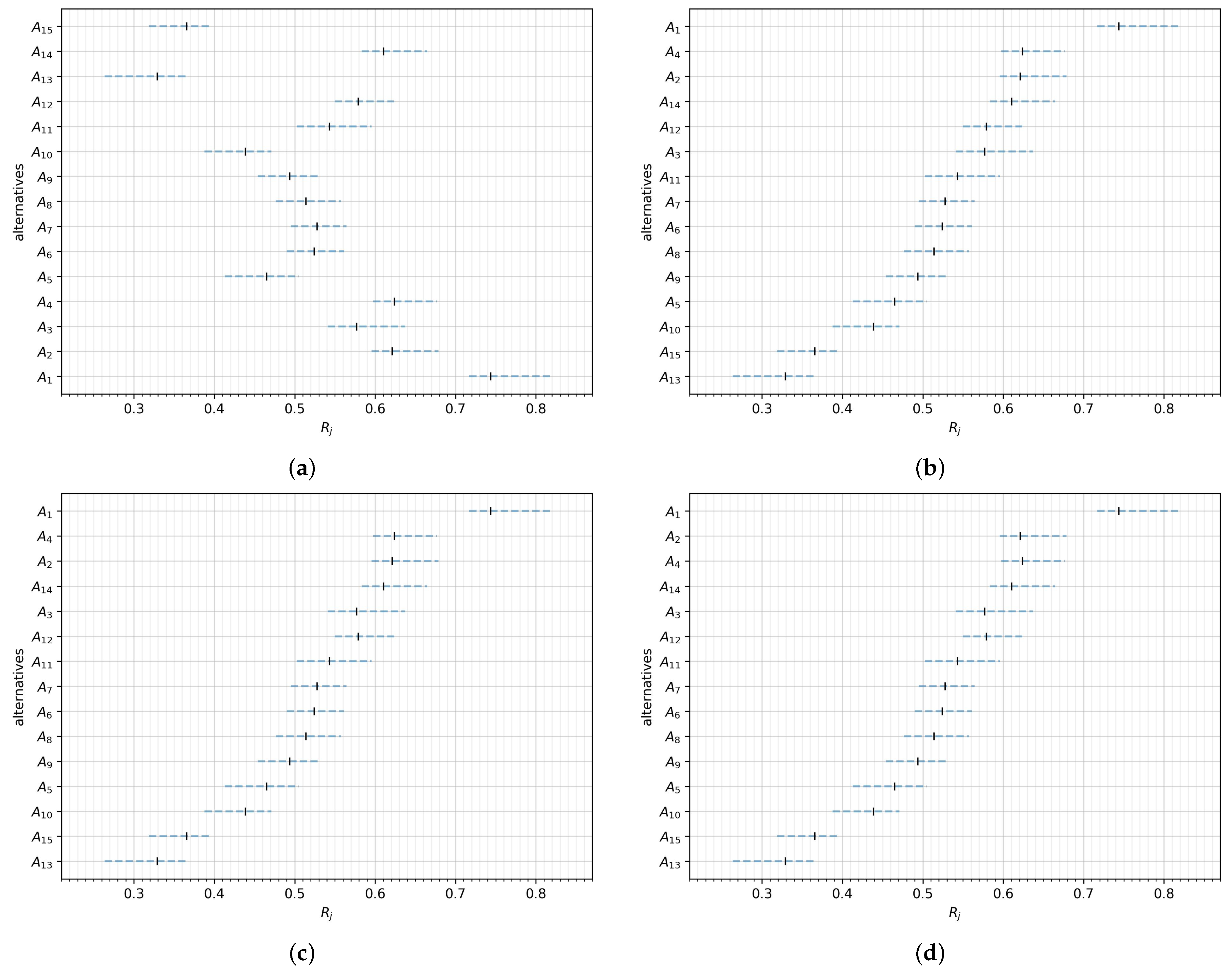
The results obtained from all the considered approaches consistently display a high degree of reliability and conformity. This is vividly depicted in Figure 4, where we visualize the relative closeness achieved through the new approach (depicted as intervals in blue) in comparison to the results obtained using the interval TOPSIS method (represented as points in black within the intervals). Two specific cases within the visualization warrant special attention.
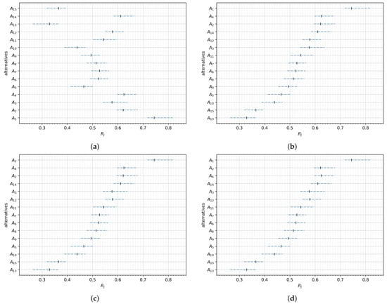
Figure 4.
Relative closeness values for alternatives. (a) Not sorted. (b) Sorted by the lower limit of . (c) Sorted by the mean of the lower and upper limit of . (d) Sorted by the upper limit of .
Firstly, the relative closeness of the interval attributed to the alternative stands out as it does not overlap with any other interval. Consequently, there is unequivocal certainty regarding its ranking position, with no room for dispute or contention with other alternatives.
Secondly, the pairs of alternatives, namely and , along with and , merit a close examination. Here, the relative closeness of the interval for alternative is fully encompassed within the interval of alternative . An analogous situation occurs with the alternatives and . Such pairs of alternatives are the only ones in which there have been changes within the rankings available using the new approach.
It is also worth noting that although each value was symmetrically expanded by the same value, the results in comparison to the interval TOPSIS method are not symmetrical. With some alternatives, for example and generally the highest-rated alternatives, crisp relative closeness is closer to the lower limit of interval relative closeness. In contrast, with the lowest-rated alternatives, such as , the value moves closer to the upper limit.
Based on the results, it can be concluded that the new approach substantially matches the interval TOPSIS. Relative closeness obtained from the interval TOPSIS never, in fact, exceeds the intervals established by the new approach. Therefore, the use of the new approach is not expected to cause inconsistencies in the results. Instead, it presents other opportunities and brings into discussion the adequacy of the original interval extension.
The results returned as intervals are in a form consistent with the input data. This provides an alternative, more relevant way to model uncertainty. It also leaves more possibilities for interpretation for the decision-maker. For example, for the data used, most alternatives are unambiguously evaluated, such as the first ranking being the same regardless of which interval limit is considered. In some other cases, the decision-maker can decide how to interpret overlapping intervals of relative closeness in the decision-making process. Thus, if the TOPSIS method is chosen to deal with interval data, the new approach may provide additional insight into the results compared to the interval TOPSIS proposed by Jahanshahloo.
5. Conclusions
Through this investigation, our primary objective is to evaluate the robustness and consistency of the results produced by these two distinct approaches and, furthermore, to elucidate how such a fundamental difference in methodology can potentially impact the decision-making process. To enable a meaningful comparison between these two methods, we propose a simple approach to represent the intervals obtained in our extension as crisp values (left bound, right bound, or midpoint). It is important to note that in our extension, each preference is explicitly expressed as an interval with defined minimum and maximum possible values. The use of crisp values is primarily for the purpose of comparison with the Jahanshahloo approach, where preference values are presented as single, noninterval numbers. In the Jahanshahloo approach, the use of single crisp values may impose limitations in capturing the inherent variability and uncertainty inherent in the decision-making process.
The paper compares two interval-based extensions of the TOPSIS method. An electric vehicle evaluation challenge was used as an example due to the relevance of the topic and possible straightforward adaptation to an MCDA problem. The two approaches are found to have high mutual compatibility. The most popular approach proposed by Jahanshahloo returns results that fall within the limits defined by the results obtained from the new approach. This suggests that the new approach could be used interchangeably with the original interval extension. However, it does not neglect the uncertain nature of the problem. In Jahanshahloo’s extension, evaluating an alternative with interval attributes by a crisp number poses the risk of eliminating other potential evaluations for that alternative. In the new approach, there is no such risk, because the interval evaluation of an alternative by definition represents the range of all possible evaluations for that alternative.
Further research directions could be to continue investigating the adequacy of the results returned by the new approach, to examine how the new approach performs on data from other domains, and to study the behavior of the new approach under different levels of uncertainty.
Author Contributions
Conceptualization, W.S.; methodology, W.S.; software, A.K.; validation, A.K., P.S., J.W., and W.S.; formal analysis, A.K., P.S., J.W., and W.S.; investigation, A.K., P.S., J.W., and W.S.; resources, A.K., P.S., J.W., and W.S.; data curation, A.K.; writing—original draft preparation, A.K. and W.S.; writing—review and editing, A.K., P.S., J.W., and W.S.; visualization, A.K. and W.S.; supervision, W.S.; project administration, A.K., P.S., J.W., and W.S.; funding acquisition, A.K., P.S., J.W., and W.S. All authors have read and agreed to the published version of the manuscript.
Funding
This research was supported by ZUT Highfliers School (Szkoła Orłów ZUT) project, co-ordinated by Dr. Piotr Sulikowski, within the framework of the program of the Minister of Education and Science (Grant No. MNiSW/2019/391/DIR/KH, POWR.03.01.00-00-P015/18), co-financed by the European Social Fund, the amount of financing PLN 2.634.975,00 and by the National Science Centre, Decision number UMO-2021/41/B/HS4/01296.
Data Availability Statement
The data presented in this study are available in article.
Acknowledgments
The authors would like to thank the editor and the anonymous reviewers, whose insightful comments and constructive suggestions helped us to significantly improve the quality of this paper.
Conflicts of Interest
The authors declare no conflict of interest.
Abbreviations
The following abbreviations are used in this manuscript:
| COMET | Characteristic Objects METhod |
| EV | Electric vehicle |
| MCDA | Multi-Criteria Decision Analysis |
| PROMETHEE | Preference Ranking Organization Method of Enrichment Evaluation |
| TOPSIS | Technique for Order Preference by Similarity to Ideal Solution |
| VIKOR | VlseKriterijumska Optimizacija I Kompromisno Resenje |
References
- Wątróbski, J.; Jankowski, J.; Ziemba, P.; Karczmarczyk, A.; Zioło, M. Generalised framework for multi-criteria method selection. Omega 2019, 86, 107–124. [Google Scholar] [CrossRef]
- Diaby, V.; Campbell, K.; Goeree, R. Multi-criteria decision analysis (MCDA) in health care: A bibliometric analysis. Oper. Res. Health Care 2013, 2, 20–24. [Google Scholar] [CrossRef]
- Huang, I.B.; Keisler, J.; Linkov, I. Multi-criteria decision analysis in environmental sciences: Ten years of applications and trends. Sci. Total Environ. 2011, 409, 3578–3594. [Google Scholar] [CrossRef] [PubMed]
- Zhou, P.; Ang, B.; Poh, K. Decision analysis in energy and environmental modeling: An update. Energy 2006, 31, 2604–2622. [Google Scholar] [CrossRef]
- Mendoza, G.A.; Martins, H. Multi-criteria decision analysis in natural resource management: A critical review of methods and new modelling paradigms. For. Ecol. Manag. 2006, 230, 1–22. [Google Scholar] [CrossRef]
- Zopounidis, C.; Doumpos, M. Multi-criteria decision aid in financial decision making: Methodologies and literature review. J. Multi-Criteria Decis. Anal. 2002, 11, 167–186. [Google Scholar] [CrossRef]
- Triantaphyllou, E. Multi-Criteria Decision Making Methods; Springer: Berlin/Heidelberg, Germany, 2000. [Google Scholar]
- Kumar, R.R.; Alok, K. Adoption of electric vehicle: A literature review and prospects for sustainability. J. Clean. Prod. 2020, 253, 119911. [Google Scholar] [CrossRef]
- Sanguesa, J.A.; Torres-Sanz, V.; Garrido, P.; Martinez, F.J.; Marquez-Barja, J.M. A review on electric vehicles: Technologies and challenges. Smart Cities 2021, 4, 372–404. [Google Scholar] [CrossRef]
- Ziemba, P. Selection of electric vehicles for the needs of sustainable transport under conditions of uncertainty—A comparative study on fuzzy MCDA methods. Energies 2021, 14, 7786. [Google Scholar] [CrossRef]
- Poullikkas, A. Sustainable options for electric vehicle technologies. Renew. Sustain. Energy Rev. 2015, 41, 1277–1287. [Google Scholar] [CrossRef]
- Wątróbski, J.; Małecki, K.; Kijewska, K.; Iwan, S.; Karczmarczyk, A.; Thompson, R.G. Multi-criteria analysis of electric vans for city logistics. Sustainability 2017, 9, 1453. [Google Scholar] [CrossRef]
- Ziemba, P. Multi-criteria stochastic selection of electric vehicles for the sustainable development of local government and state administration units in Poland. Energies 2020, 13, 6299. [Google Scholar] [CrossRef]
- Aiello, G.; Quaranta, S.; Certa, A.; Inguanta, R. Optimization of urban delivery systems based on electric assisted cargo bikes with modular battery size, taking into account the service requirements and the specific operational context. Energies 2021, 14, 4672. [Google Scholar] [CrossRef]
- Yang, X.G.; Liu, T.; Ge, S.; Rountree, E.; Wang, C.Y. Challenges and key requirements of batteries for electric vertical takeoff and landing aircraft. Joule 2021, 5, 1644–1659. [Google Scholar] [CrossRef]
- Biswas, T.K.; Das, M.C. Selection of commercially available electric vehicle using fuzzy AHP-MABAC. J. Inst. Eng. (India) Ser. C 2019, 100, 531–537. [Google Scholar] [CrossRef]
- Ecer, F. A consolidated MCDM framework for performance assessment of battery electric vehicles based on ranking strategies. Renew. Sustain. Energy Rev. 2021, 143, 110916. [Google Scholar] [CrossRef]
- Kim, S.; Choi, J.; Yi, Y.; Kim, H. Analysis of Influencing Factors in Purchasing Electric Vehicles Using a Structural Equation Model: Focused on Suwon City. Sustainability 2022, 14, 4744. [Google Scholar] [CrossRef]
- Peng, H.; Qin, D.; Hu, J.; Fu, C. Synthesis and analysis method for powertrain configuration of single motor hybrid electric vehicle. Mech. Mach. Theory 2020, 146, 103731. [Google Scholar] [CrossRef]
- Zhang, B.; Zhang, J.; Shen, T. Optimal control design for comfortable-driving of hybrid electric vehicles in acceleration mode. Appl. Energy 2022, 305, 117885. [Google Scholar] [CrossRef]
- Huda, N.; Kaleg, S.; Hapid, A.; Kurnia, M.R.; Budiman, A.C. The influence of the regenerative braking on the overall energy consumption of a converted electric vehicle. SN Appl. Sci. 2020, 2, 606. [Google Scholar] [CrossRef]
- Holmberg, K.; Erdemir, A. The impact of tribology on energy use and CO2 emission globally and in combustion engine and electric cars. Tribol. Int. 2019, 135, 389–396. [Google Scholar] [CrossRef]
- Zhang, C.; Yang, F.; Ke, X.; Liu, Z.; Yuan, C. Predictive modeling of energy consumption and greenhouse gas emissions from autonomous electric vehicle operations. Appl. Energy 2019, 254, 113597. [Google Scholar] [CrossRef]
- Liang, X.; Wu, X.; Liao, H. A gained and lost dominance score II method for modelling group uncertainty: Case study of site selection of electric vehicle charging stations. J. Clean. Prod. 2020, 262, 121239. [Google Scholar] [CrossRef]
- Sun, Z.; Wen, Z.; Zhao, X.; Yang, Y.; Li, S. Real-world driving cycles adaptability of electric vehicles. World Electr. Veh. J. 2020, 11, 19. [Google Scholar] [CrossRef]
- Ziemba, P. Monte Carlo simulated data for multi-criteria selection of city and compact electric vehicles in Poland. Data Brief 2021, 36, 107118. [Google Scholar] [CrossRef]
- Bączkiewicz, A.; Wątróbski, J. Crispyn—A Python library for determining criteria significance with objective weighting methods. SoftwareX 2022, 19, 101166. [Google Scholar] [CrossRef]
- Josijević, M.; Živković, D.; Gordić, D.; Končalović, D.; Vukašinović, V. The analysis of commercially available electric cars. Mobil. Veh. Mech. 2022, 48, 19–36. [Google Scholar] [CrossRef]
- Danielis, R.; Rotaris, L.; Giansoldati, M.; Scorrano, M. Drivers’ preferences for electric cars in Italy. Evidence from a country with limited but growing electric car uptake. Transp. Res. Part A Policy Pract. 2020, 137, 79–94. [Google Scholar] [CrossRef]
- Liu, Q. TOPSIS Model for evaluating the corporate environmental performance under intuitionistic fuzzy environment. Int. J. Knowl.-Based Intell. Eng. Syst. 2022, 26, 149–157. [Google Scholar] [CrossRef]
- Yeh, C.H. The selection of multiattribute decision making methods for scholarship student selection. Int. J. Sel. Assess. 2003, 11, 289–296. [Google Scholar] [CrossRef]
- Ashrafzadeh, M.; Rafiei, F.M.; Isfahani, N.M.; Zare, Z. Application of fuzzy TOPSIS method for the selection of Warehouse Location: A Case Study. Interdiscip. J. Contemp. Res. Bus. 2012, 3, 655–671. [Google Scholar]
- Shih, H.S.; Shyur, H.J.; Lee, E.S. An extension of TOPSIS for group decision making. Math. Comput. Model. 2007, 45, 801–813. [Google Scholar] [CrossRef]
- Behzadian, M.; Otaghsara, S.K.; Yazdani, M.; Ignatius, J. A state-of the-art survey of TOPSIS applications. Expert Syst. Appl. 2012, 39, 13051–13069. [Google Scholar] [CrossRef]
- Li, Y.; Cai, Q.; Wei, G. PT-TOPSIS methods for multi-attribute group decision making under single-valued neutrosophic sets. Int. J. Knowl.-Based Intell. Eng. Syst. 2023, 27, 1–18. [Google Scholar] [CrossRef]
- Ding, L.; Shao, Z.; Zhang, H.; Xu, C.; Wu, D. A comprehensive evaluation of urban sustainable development in China based on the TOPSIS-entropy method. Sustainability 2016, 8, 746. [Google Scholar] [CrossRef]
- Guo, S.; Zhao, H. Optimal site selection of electric vehicle charging station by using fuzzy TOPSIS based on sustainability perspective. Appl. Energy 2015, 158, 390–402. [Google Scholar] [CrossRef]
- Memari, A.; Dargi, A.; Jokar, M.R.A.; Ahmad, R.; Rahim, A.R.A. Sustainable supplier selection: A multi-criteria intuitionistic fuzzy TOPSIS method. J. Manuf. Syst. 2019, 50, 9–24. [Google Scholar] [CrossRef]
- Wątróbski, J.; Bączkiewicz, A.; Ziemba, E.; Sałabun, W. Sustainable cities and communities assessment using the DARIA-TOPSIS method. Sustain. Cities Soc. 2022, 83, 103926. [Google Scholar] [CrossRef]
- Dinçer, H.; Yüksel, S. Financial sector-based analysis of the G20 economies using the integrated decision-making approach with DEMATEL and TOPSIS. In Proceedings of the Emerging Trends in Banking and Finance: 3rd International Conference on Banking and Finance Perspectives, North Cyprus, Turkey, 25–27 April 2018; Springer: Berlin/Heidelberg, Germany, 2018; pp. 210–223. [Google Scholar]
- Perçin, S.; Aldalou, E. Financial performance evaluation of Turkish airline companies using integrated fuzzy AHP fuzzy TOPSIS model. Uluslararası İktis. İdari İncel. Derg. 2018, 583–598. [Google Scholar] [CrossRef]
- ÜNVAN, Y.A. Financial performance analysis of banks with TOPSIS and fuzzy TOPSIS approaches. Gazi Univ. J. Sci. 2020, 33, 904–923. [Google Scholar] [CrossRef]
- Ervural, B.C.; Zaim, S.; Demirel, O.F.; Aydin, Z.; Delen, D. An ANP and fuzzy TOPSIS-based SWOT analysis for Turkey’s energy planning. Renew. Sustain. Energy Rev. 2018, 82, 1538–1550. [Google Scholar] [CrossRef]
- Musbah, H.; Ali, G.; Aly, H.H.; Little, T.A. Energy management using multi-criteria decision making and machine learning classification algorithms for intelligent system. Electr. Power Syst. Res. 2022, 203, 107645. [Google Scholar] [CrossRef]
- Solangi, Y.A.; Tan, Q.; Mirjat, N.H.; Ali, S. Evaluating the strategies for sustainable energy planning in Pakistan: An integrated SWOT-AHP and Fuzzy-TOPSIS approach. J. Clean. Prod. 2019, 236, 117655. [Google Scholar] [CrossRef]
- Celik, E.; Akyuz, E. An interval type-2 fuzzy AHP and TOPSIS methods for decision-making problems in maritime transportation engineering: The case of ship loader. Ocean Eng. 2018, 155, 371–381. [Google Scholar] [CrossRef]
- Kaewfak, K.; Huynh, V.N.; Ammarapala, V.; Charoensiriwath, C. A fuzzy AHP-TOPSIS approach for selecting the multimodal freight transportation routes. In Proceedings of the Knowledge and Systems Sciences: 20th International Symposium, KSS 2019, Da Nang, Vietnam, 29 November–1 December 2019; Proceedings 20. Springer: Berlin/Heidelberg, Germany, 2019; pp. 28–46. [Google Scholar]
- Wu, X.; Zhang, C.; Yang, L. Evaluation and selection of transportation service provider by TOPSIS method with entropy weight. Therm. Sci. 2021, 25, 1483–1488. [Google Scholar] [CrossRef]
- Sun, F.; Lu, F.; Bi, H.; Yu, C. FAHP based evaluation of IT Outsourcing risk. In Proceeding of the 11th World Congress on Intelligent Control and Automation, Shenyang, China, 29 June–4 July 2014; IEEE: Piscataway, NJ, USA, 2014; pp. 602–604. [Google Scholar]
- Zhao, M.; Qin, S.-s.; Li, Q.-w.; Lu, F.-q.; Shen, Z. The likelihood ranking methods for interval type-2 fuzzy sets considering risk preferences. Math. Probl. Eng. 2015, 2015, 680635. [Google Scholar] [CrossRef]
- Jin, L.; Yager, R.R.; Chen, Z.S.; Špirková, J.; Mesiar, R. Interval and BUI type basic uncertain information in multi-sources evaluation and rules based decision making. Int. J. Gen. Syst. 2023, 52, 443–454. [Google Scholar] [CrossRef]
- Groothuis-Oudshoorn, C.G.; Broekhuizen, H.; van Til, J. Dealing with uncertainty in the analysis and reporting of MCDA. In Multi-Criteria Decision Analysis to Support Healthcare Decisions; Springer: Cham, Switzerland, 2017; pp. 67–85. [Google Scholar]
- Stewart, T. Dealing with uncertainties in MCDA. In Multiple Criteria Decision Analysis: State of the Art Surveys; Springer: New York, NY, USA, 2005; pp. 445–466. [Google Scholar]
- Hyde, K.; Maier, H.R.; Colby, C. Incorporating uncertainty in the PROMETHEE MCDA method. J. Multi-Criteria Decis. Anal. 2003, 12, 245–259. [Google Scholar] [CrossRef]
- Chen, T.Y. A novel VIKOR method with an application to multiple criteria decision analysis for hospital-based post-acute care within a highly complex uncertain environment. Neural Comput. Appl. 2019, 31, 3969–3999. [Google Scholar] [CrossRef]
- Sałabun, W.; Karczmarczyk, A.; Wątróbski, J.; Jankowski, J. Handling data uncertainty in decision making with COMET. In Proceedings of the 2018 IEEE Symposium Series on Computational Intelligence (SSCI), Bengaluru, India, 18–21 November 2018; IEEE: Piscataway, NJ, USA, 2018; pp. 1478–1484. [Google Scholar]
- Jin, L.S.; Chen, Z.S.; Yager, R.R.; Langari, R. Interval Type Interval and Cognitive Uncertain Information in Information Fusion and Decision Making. Int. J. Comput. Intell. Syst. 2023, 16, 60. [Google Scholar] [CrossRef]
- Boczek, M.; Jin, L.; Kaluszka, M. The interval-valued Choquet-Sugeno-like operator as a tool for aggregation of interval-valued functions. Fuzzy Sets Syst. 2022, 448, 35–48. [Google Scholar] [CrossRef]
- Palczewski, K.; Sałabun, W. The fuzzy TOPSIS applications in the last decade. Procedia Comput. Sci. 2019, 159, 2294–2303. [Google Scholar] [CrossRef]
- Jahanshahloo, G.R.; Lotfi, F.H.; Izadikhah, M. An algorithmic method to extend TOPSIS for decision-making problems with interval data. Appl. Math. Comput. 2006, 175, 1375–1384. [Google Scholar] [CrossRef]
- Jahanshahloo, G.R.; Lotfi, F.H.; Davoodi, A. Extension of TOPSIS for decision-making problems with interval data: Interval efficiency. Math. Comput. Model. 2009, 49, 1137–1142. [Google Scholar] [CrossRef]
- Jahanshahloo, G.R.; Khodabakhshi, M.; Lotfi, F.H.; Goudarzi, M.M. A cross-efficiency model based on super-efficiency for ranking units through the TOPSIS approach and its extension to the interval case. Math. Comput. Model. 2011, 53, 1946–1955. [Google Scholar] [CrossRef]
- Dymova, L.; Sevastjanov, P.; Tikhonenko, A. A direct interval extension of TOPSIS method. Expert Syst. Appl. 2013, 40, 4841–4847. [Google Scholar] [CrossRef]
- Kaczyńska, A.; Gandotra, N.; Sałabun, W. A new approach to dealing with interval data in the TOPSIS method. Procedia Comput. Sci. 2022, 207, 4545–4555. [Google Scholar] [CrossRef]
- Sałabun, W.; Wątróbski, J.; Shekhovtsov, A. Are MCDA methods benchmarkable? A comparative study of TOPSIS, VIKOR, COPRAS, and PROMETHEE II methods. Symmetry 2020, 12, 1549. [Google Scholar] [CrossRef]
- Sałabun, W.; Urbaniak, K. A new coefficient of rankings similarity in decision-making problems. In Proceedings of the Computational Science–ICCS 2020: 20th International Conference, Amsterdam, The Netherlands, 3–5 June 2020; Proceedings, Part II 20. Springer: Berlin/Heidelberg, Germany, 2020; pp. 632–645. [Google Scholar]
- Dwivedi, P.P.; Sharma, D.K. Evaluation and ranking of battery electric vehicles by Shannon’s entropy and TOPSIS methods. Math. Comput. Simul. 2023, 212, 457–474. [Google Scholar] [CrossRef]

Disclaimer/Publisher’s Note: The statements, opinions and data contained in all publications are solely those of the individual author(s) and contributor(s) and not of MDPI and/or the editor(s). MDPI and/or the editor(s) disclaim responsibility for any injury to people or property resulting from any ideas, methods, instructions or products referred to in the content. |
© 2023 by the authors. Licensee MDPI, Basel, Switzerland. This article is an open access article distributed under the terms and conditions of the Creative Commons Attribution (CC BY) license (https://creativecommons.org/licenses/by/4.0/).