
Multi-Objective Decision Approach for Optimal Real-Time Switching Sequence of Network Reconfiguration Realizing Maximum Load Capacity


Abstract
:1. Introduction
- The first contribution is to find the optimal distribution network reconfiguration (DNR) simultaneously with optimal distributed generation location and sizing (DG-LS), which achieves the maximum active and reactive load capacities of the distribution network (DN) in planning mode. Most of the existing literature has focused on finding the minimum power loss.
- The unique contribution of this paper is to present an efficient methodology to find the optimal real-time switching sequence order (SSO), which allows the network to change its topography from the initial configuration to the optimal configuration without violating the constraints on operation mode. This is achieved based on the optimal solution obtained from the first contribution. Most of the existing literature has focused on finding the optimal configuration of the network in planning mode.
2. Mathematical Formulation and Constraints
- Power Constraints
- The power injection constraint.
- The power balance constraint.
- 2.
- DG Constraintswhere and are the DG the acceptable upper and lower limits, respectively.
- 3.
- Voltage Constraintswhere Vbus is the voltage bus, and VMin and VMax are the voltage minimum (Min) and maximum (Max) values, respectively. Any bus voltage must be between 0.95 p.u and 1.05 p.u (±5% of rated value) [48].VMin ≤ Vbus ≤ Vmax
- 4.
- Distribution Topology Form Constraints
- 5.
- Load Constraint
- 6.
- Maximum Load Capacity Factor Constraints
3. Proposed Approach
3.1. Simultaneous Optimal DNR with DG Location and Sizing for MLC
3.1.1. Analytic Hierarchy Process (AHP)
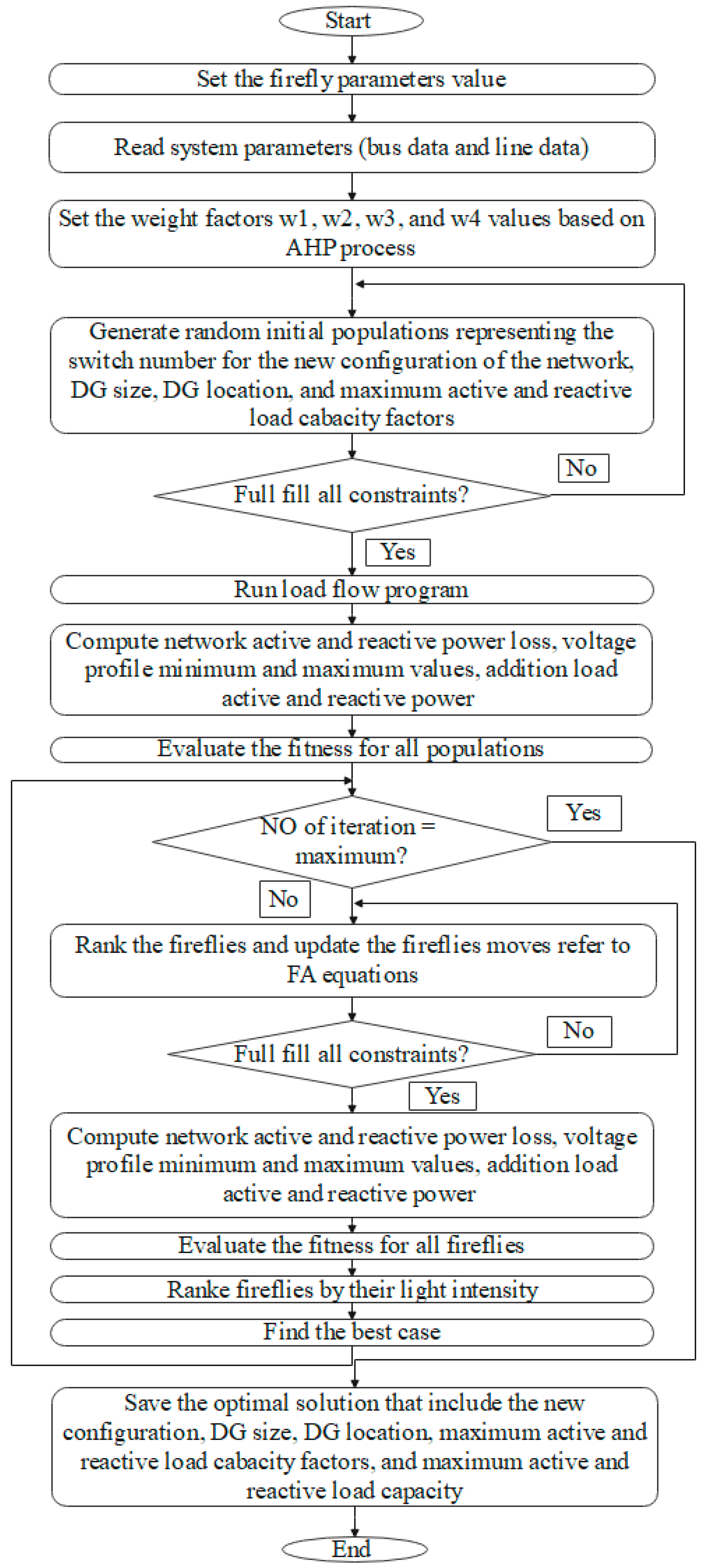
3.1.2. Firefly (FA)
- Determine the FA parameters, iteration number, and initial population size.
- Set the network parameters like PL and QL load of the buses, resistance, reactance values of the lines, and initial values of the bus’s voltages.
- Mark the fitness weight factors based on the AHP approach.
- Generate simultaneous random network initial populations (X) which fulfill all constraints and limitations. X indicates the network tie switches number (S) for the new configuration, DG location (DGL), DG sizing (DGS), and MLC factors (λ).where n is the tie switch number; q is the DG number; and m is the initial population size.
- Run the load flow code which is based on the Newton–Raphson method. Then, evaluate the Ploss and Qloss values, maximum PL and QL values of each bus, and Max and Min values of the bus’s voltages for the entire network. Then, calculate the fitness.
- Sort the populations from low to high fitness. Save the best light intensity which represents the fitness minimum value.
- Start the mutation iteration loop by evaluating the fitness value for each population generated on matrix X related to Equation (1).
- Sort the populations from low to high fitness based on their light intensity. Save the best light intensity which represents the fitness minimum value.
- Update the elements of matrix X based on the FA optimization considering all limitations and constraints based on the following equations:where is the attractiveness when ; is the two FAs’ space; and is the coefficient of the light absorption.where is the cartesian space between the and FAs, which represents the matrix rows; is the parameter’s optimized number; and and represent a component of the cartesian coordinates and of the FAs and , respectively.where the initial term is the movement of FAs, where is attracted to the brighter ; the next term is affected by the attraction; the final term represents the random parameter related to .
- Rank the updated movement from low to high fitness.
- Repeat the above steps from 5 to 9 until reaching the maximum iteration.
- Stop the approach and output the final optimum solution, which represents the network’s new configuration, the DG’s locations, the DG’s sizing, the MLC factors, the fitness value, IVD, the maximum PL and QL load for all buses, and the minimum Ploss and Qloss of the network.
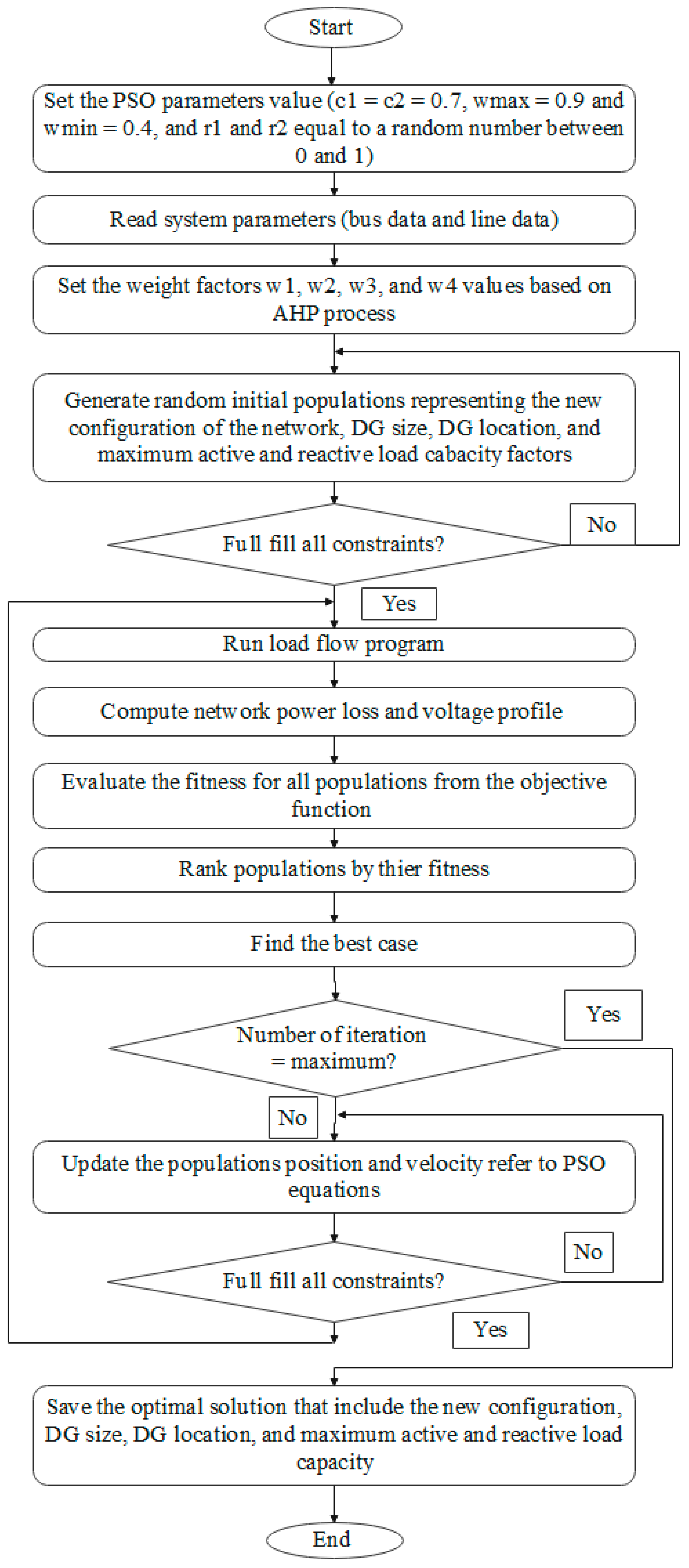
3.1.3. Particle Swarm Optimization (PSO)
- Determine the PSO parameters, iteration number, and initialization population size.
- The population stage is the same as in the FA approach (step 2 to step 6).
- Start the mutation iteration loop by evaluating the fitness value for each population generated on matrix X related to Equation (1).
- Sort the populations from low to high fitness based on their light intensity. Save the best light intensity, which represents the fitness minimum value.
- Update the particle position and velocity of matrix X related to its own searching experience and other particle experience , considering all limitations and constraints. The update of the particles’ velocity and position is conducted based on the following equations:where and are the particle current position at iteration and , respectively; and are particle ’s current velocity at iteration and , respectively; and are the PSO weighting factors; and are a random number; and are the initial Max and Min weight, respectively; and and are the current and maximum iteration number, respectively.
- Rank the updated movement from low to high fitness.
- Repeat the above steps, from 4 to 6, until reaching the maximum iteration.
- Stop the approach and output the final optimum solution, which represents the network’s new configuration, DG-LS, the MLC factors, the fitness value, IVD, the maximum PL and QL load for all buses, and the minimum Ploss and Qloss of the network.
3.2. Optimal Switching Sequence Order (SSO)
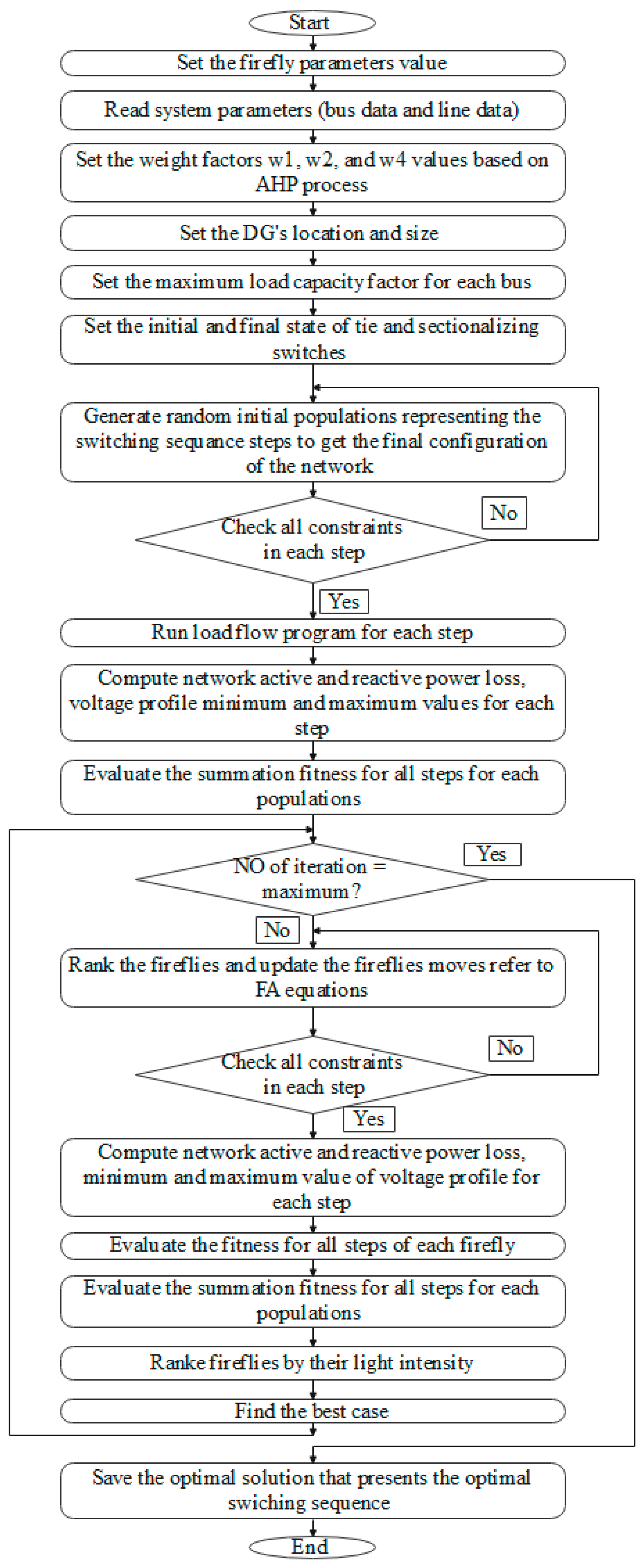
3.2.1. Firefly
- Determine the FA parameters, iteration number, and initial population size.
- Set the network parameters like active and reactive power load of the buses, resistance, reactance values of the lines, and initial values of the bus’s voltages.
- Mark the fitness weight factors based on the AHP approach.
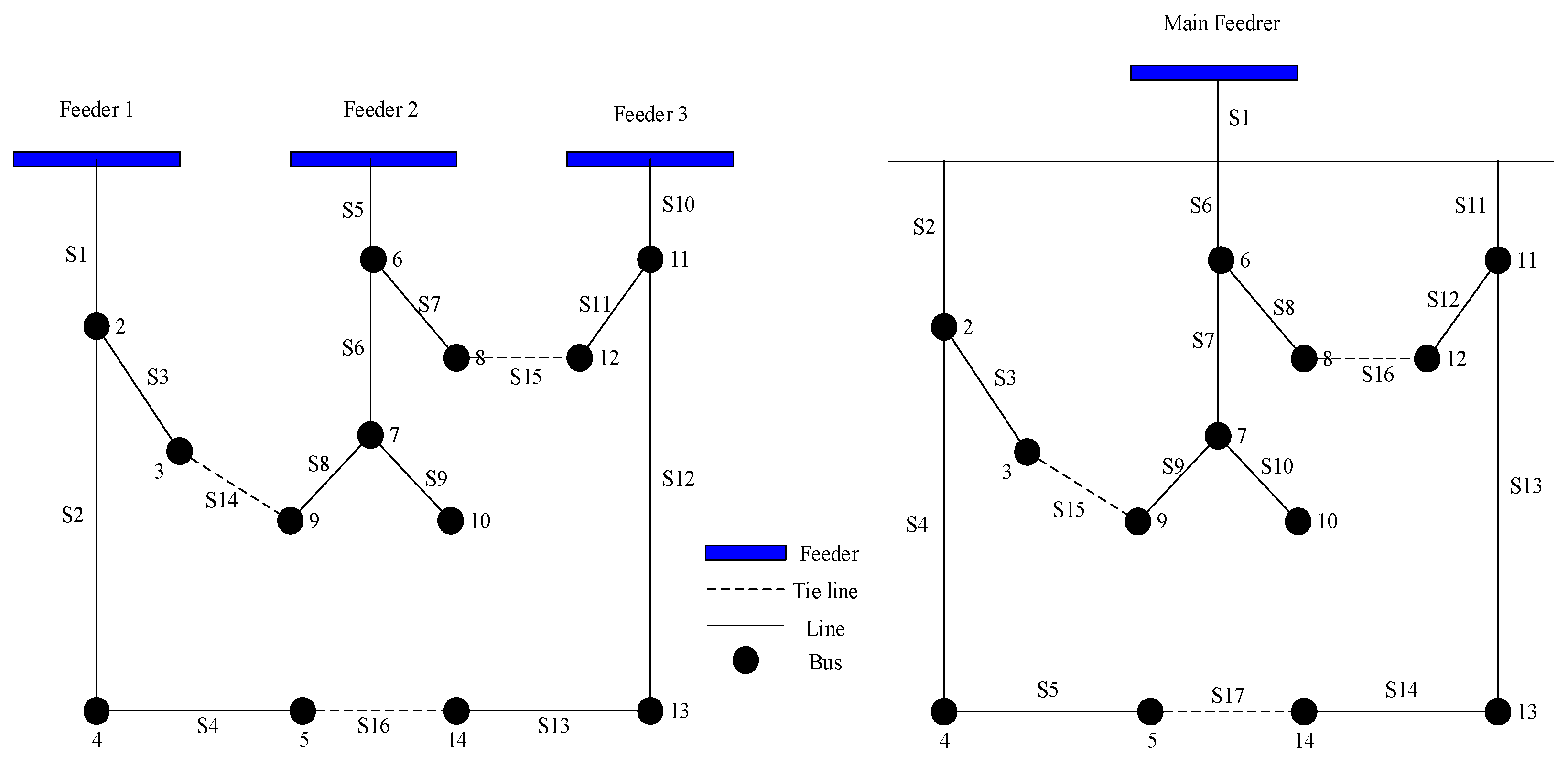
- Set the initial (original) configuration of the distribution network.
- Identify the final (optimal) configuration of the distribution network, the location and size of the DGs, and the MLC factors obtained from the reconfiguration process (presented in Section 3.1 (B)).
- Generate random network initial populations (x). x indicates the switching sequence order (SSO) which transfers the network from the initial configuration to the optimal configuration without violating the constraints of the voltage.where and are the switches to be closed and open during the SSO process, respectively, and z is the number of steps needed to change the form of the network from initial to optimal.
- Evaluate the Ploss and Qloss and the IVD for each step during the SSO process for each population.
- Calculate the fitness value for each step during the SSO process for each population.
- Sum the total fitness for all steps for each population in matrix x.
- Sort the populations from low to high fitness. Save the best light intensity, which represents the total fitness minimum value.
- Start the mutation iteration loop by evaluating the total fitness value for each population in matrix x.
- Update the elements of matrix x based on the FA optimization, considering all limitations and constraints based on Equations (17)–(19).
- Rank the updated movement from low to high total fitness.
- Repeat the above steps, from 12 to 14, until reaching the maximum iteration.
- Stop the approach and output the final optimum solution that represents the optimal switching sequence order (SSO), which transfers the network from the initial configuration to the optimal configuration, minimum Ploss and Qloss of the network, and best IVD. The function of FA is illustrated in Figure 5 in a simple flowchart for solving the proposed strategy of the SSO process.
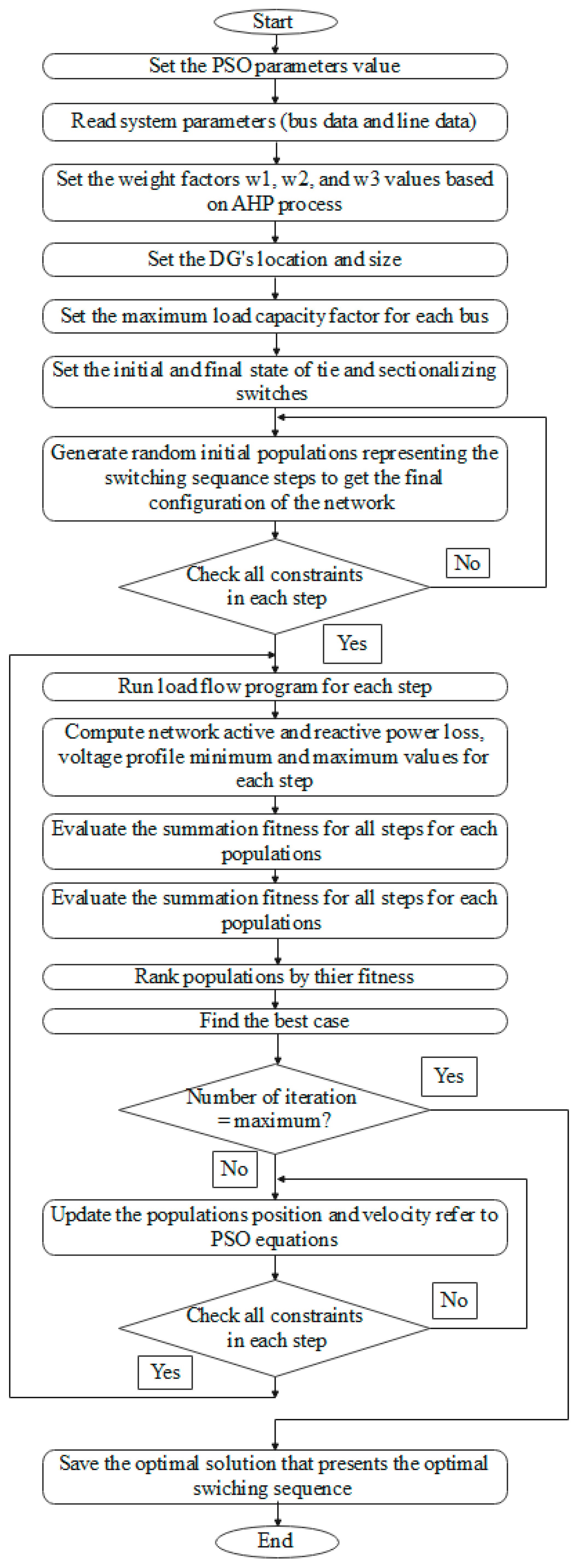
3.2.2. PSO
- Determine the PSO parameters, iteration number, and initial population size.
- Repeat steps 2 to 4 as in FA.
- Identify the final (optimal) configuration of the distribution network, the location and size of the DGs, and the MLC factors obtained from the reconfiguration process (presented in Section 3.1 (C)).
- The population stage is the same as that in the FA approach (steps 6 to 10).
- Start the mutation iteration loop by evaluating the total fitness value for each population in matrix x.
- Update the elements of matrix x based on the PSO optimization considering all limitations and constraints based on Equations (20)–(22).
- Rank the updated movement from low to high total fitness.
- Repeat the above steps, from 5 to 7, until reaching the maximum iteration.
- Stop the approach and output the final optimum solution that represents the optimal switching sequence order (SSO), which transfers the network from the initial configuration to the optimal configuration, minimum Ploss and Qloss of the network, and best IVD. The function of PSO is illustrated in Figure 6 in a simple flowchart for solving the proposed strategy of the SSO process.
4. Results and Discussion
4.1. Influence of DNR and DG-LS on Network Performance
4.1.1. Impact of DNR and DG-LS on Power Loss
4.1.2. Impact of DNR and DG-LS on Power Load
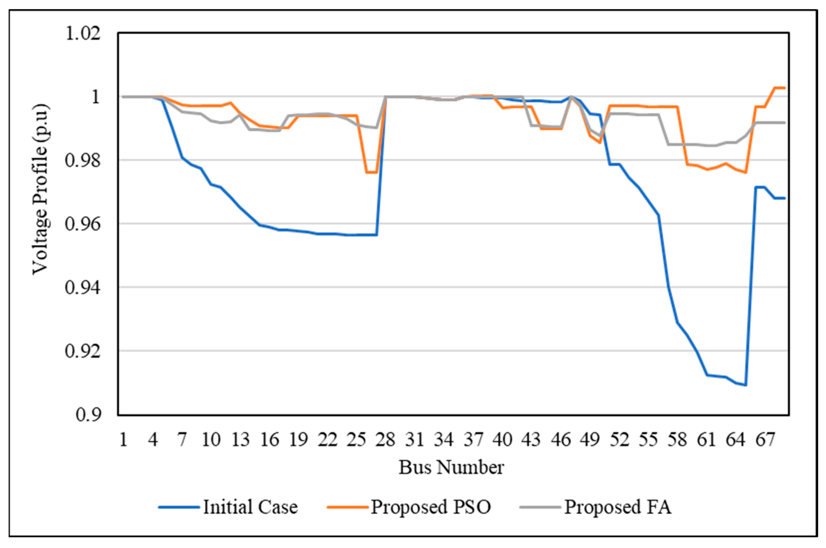
4.1.3. Impact of DNR and DG-LS on Voltage Profile
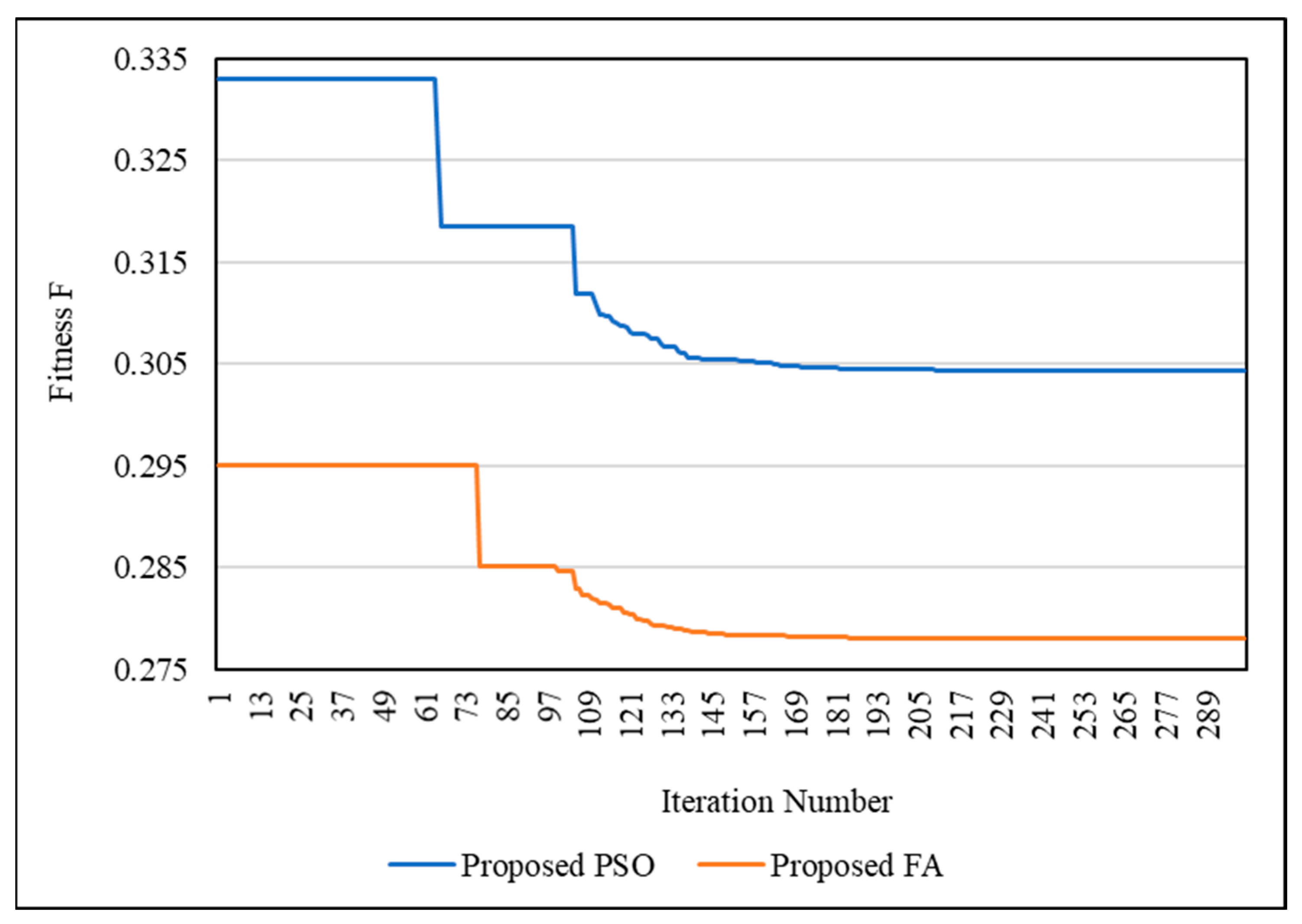
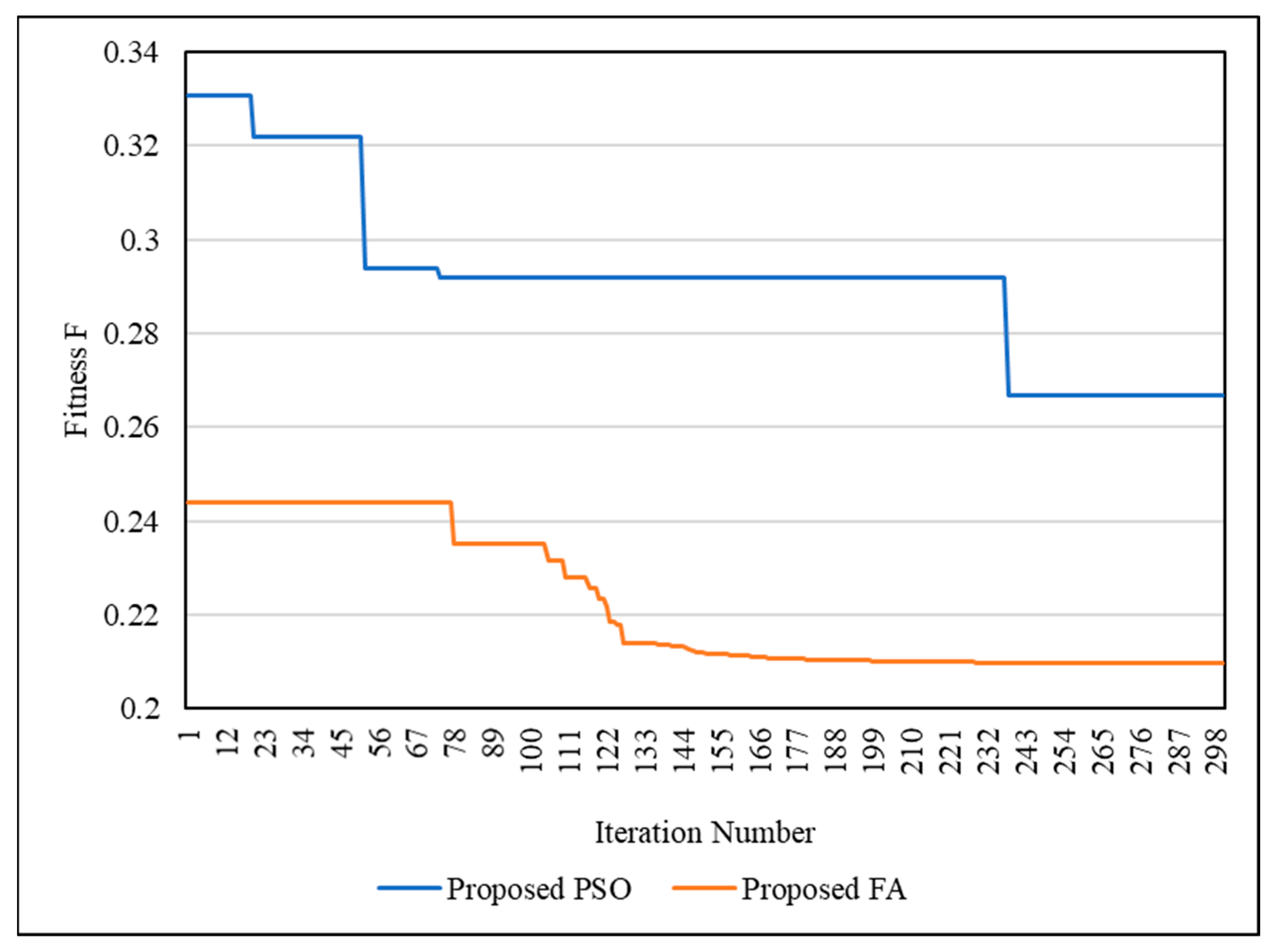
4.1.4. Impact of DNR and DG-LS on Optimization Performance
4.2. Influence of SSO on Network Performance
4.2.1. Impact of SSO on Power Loss
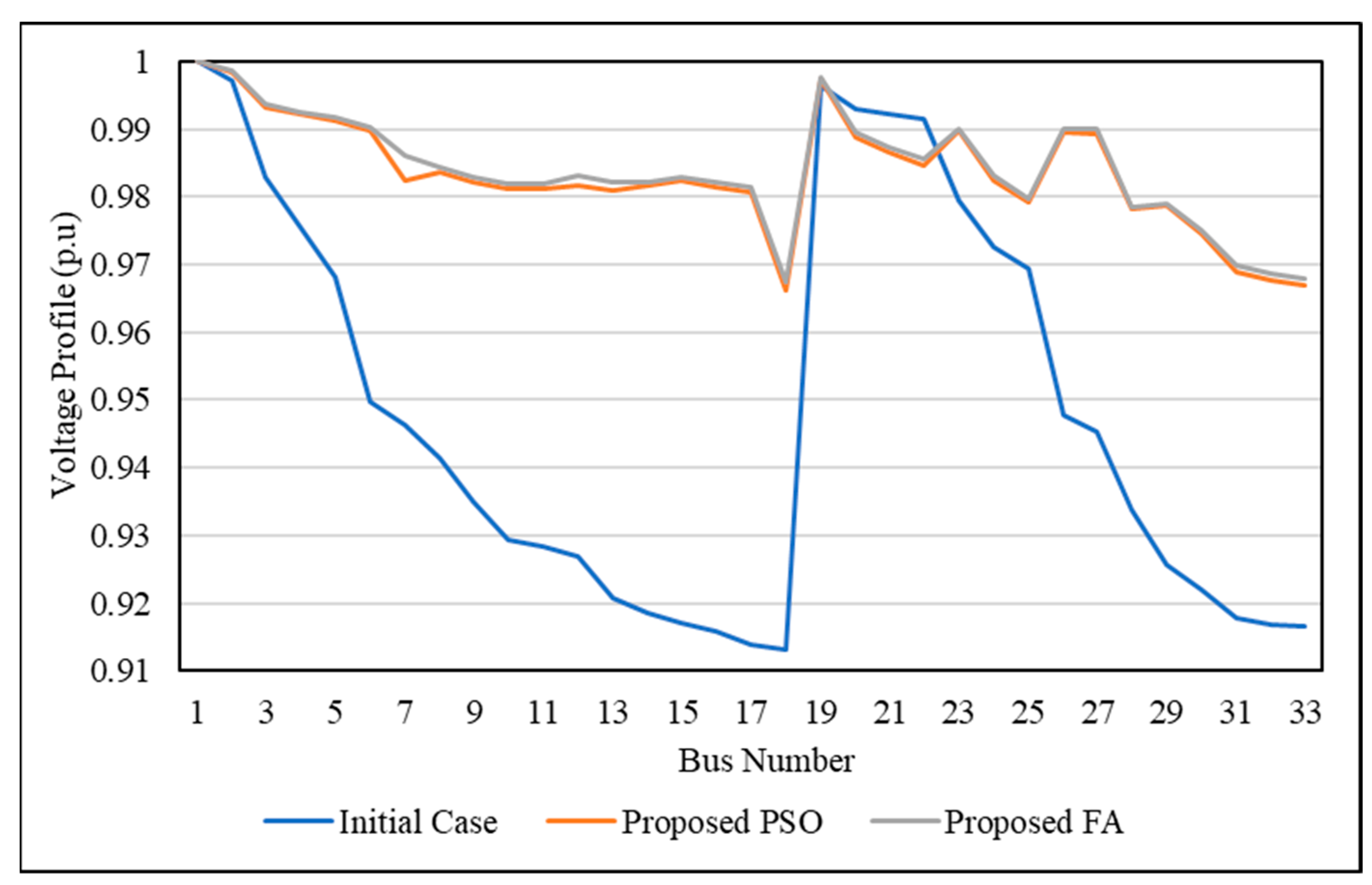
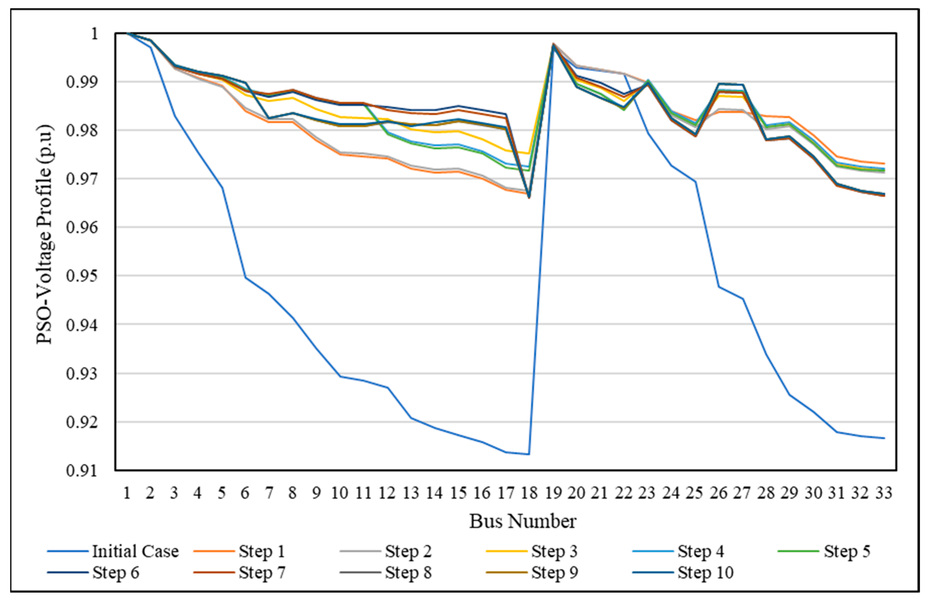
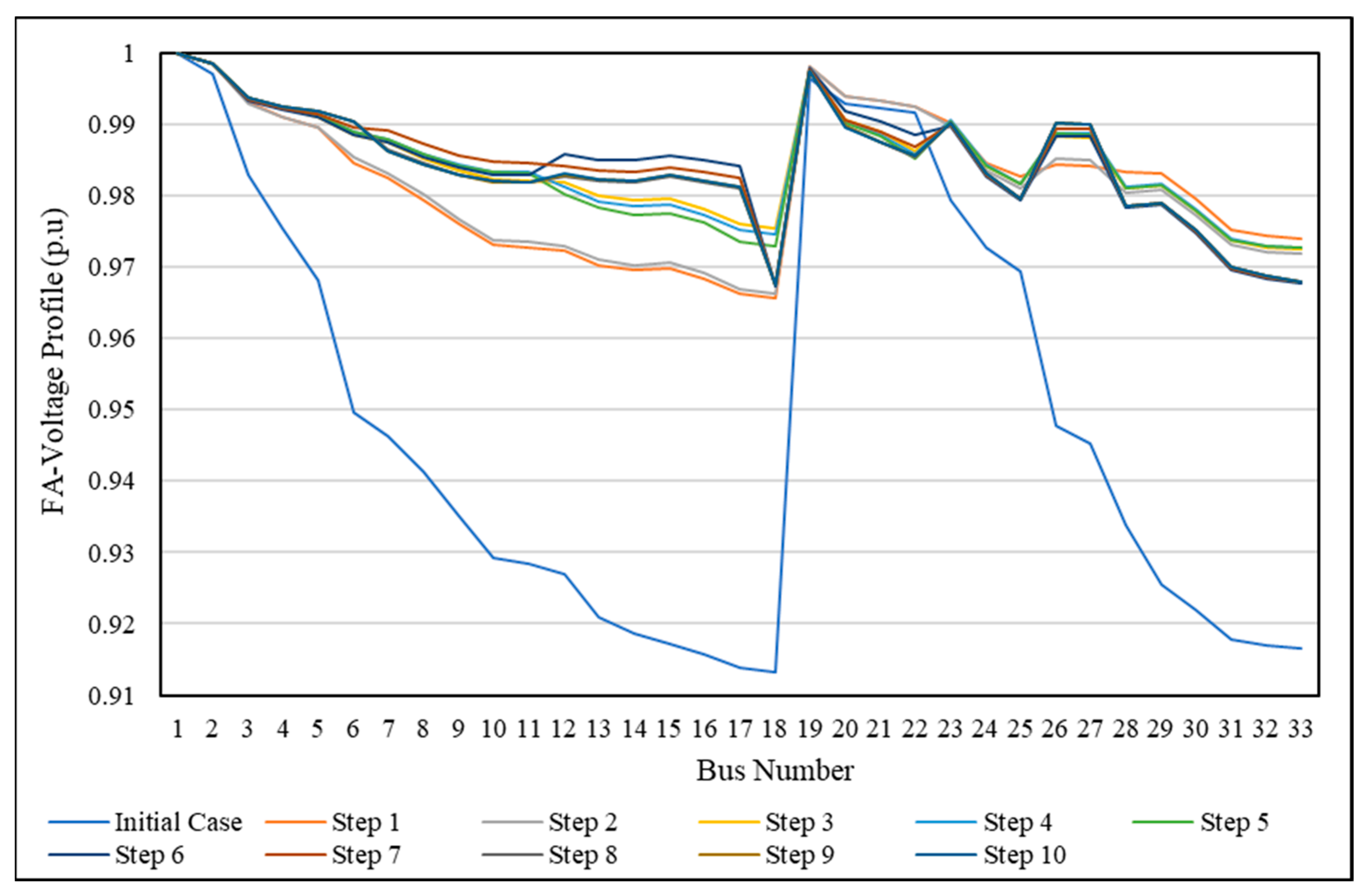
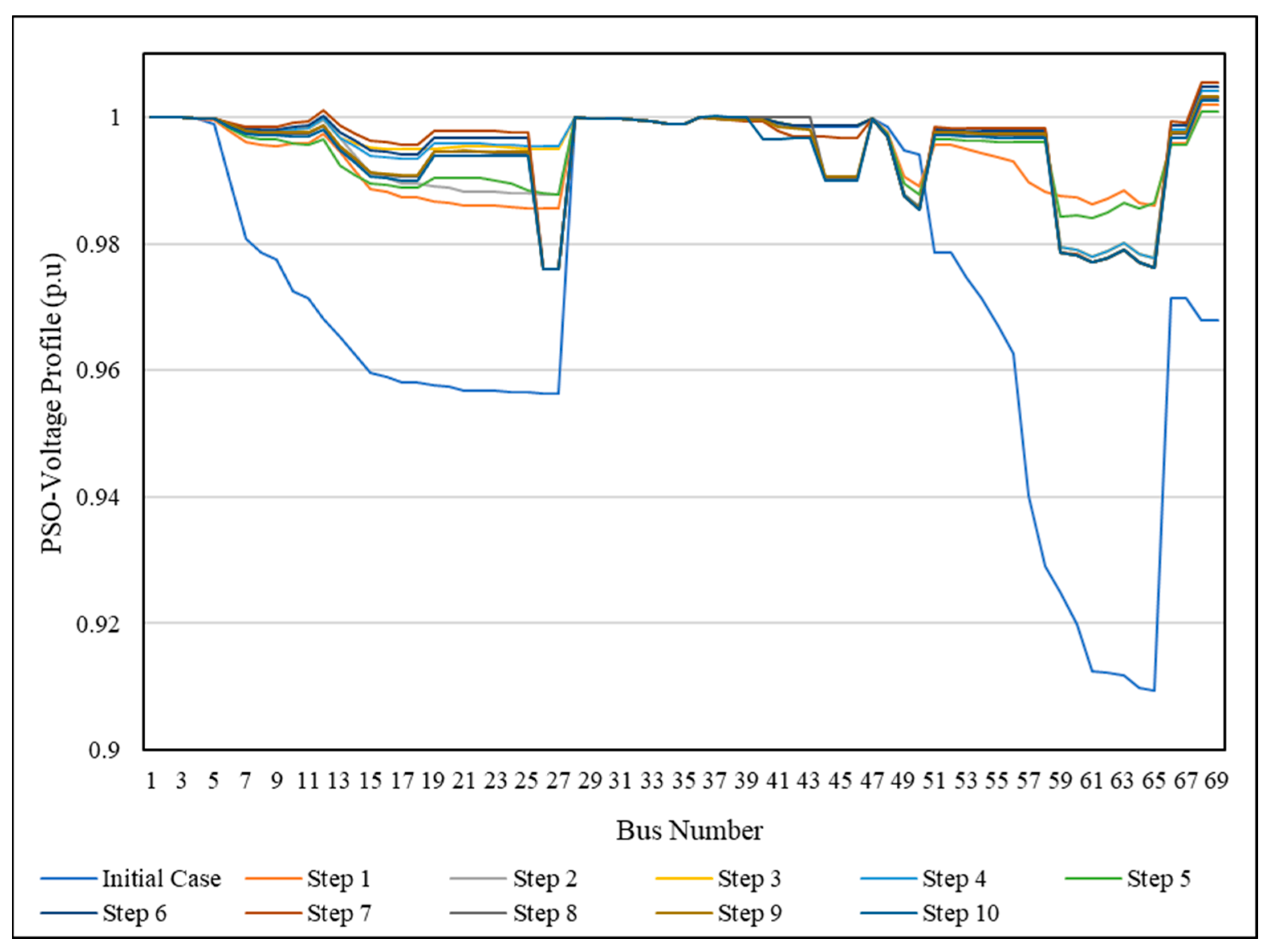
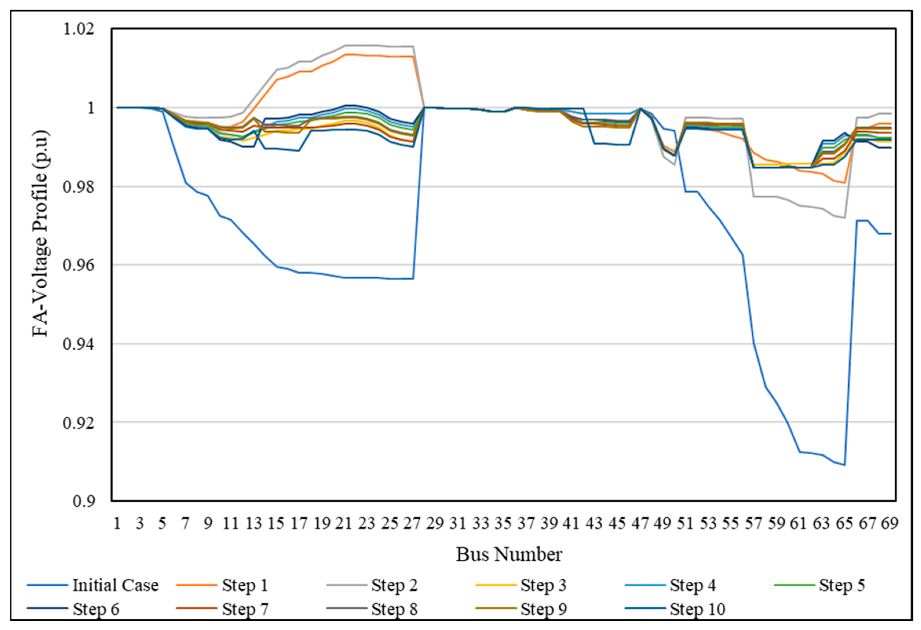
4.2.2. Impact of SSO on Voltage Profile
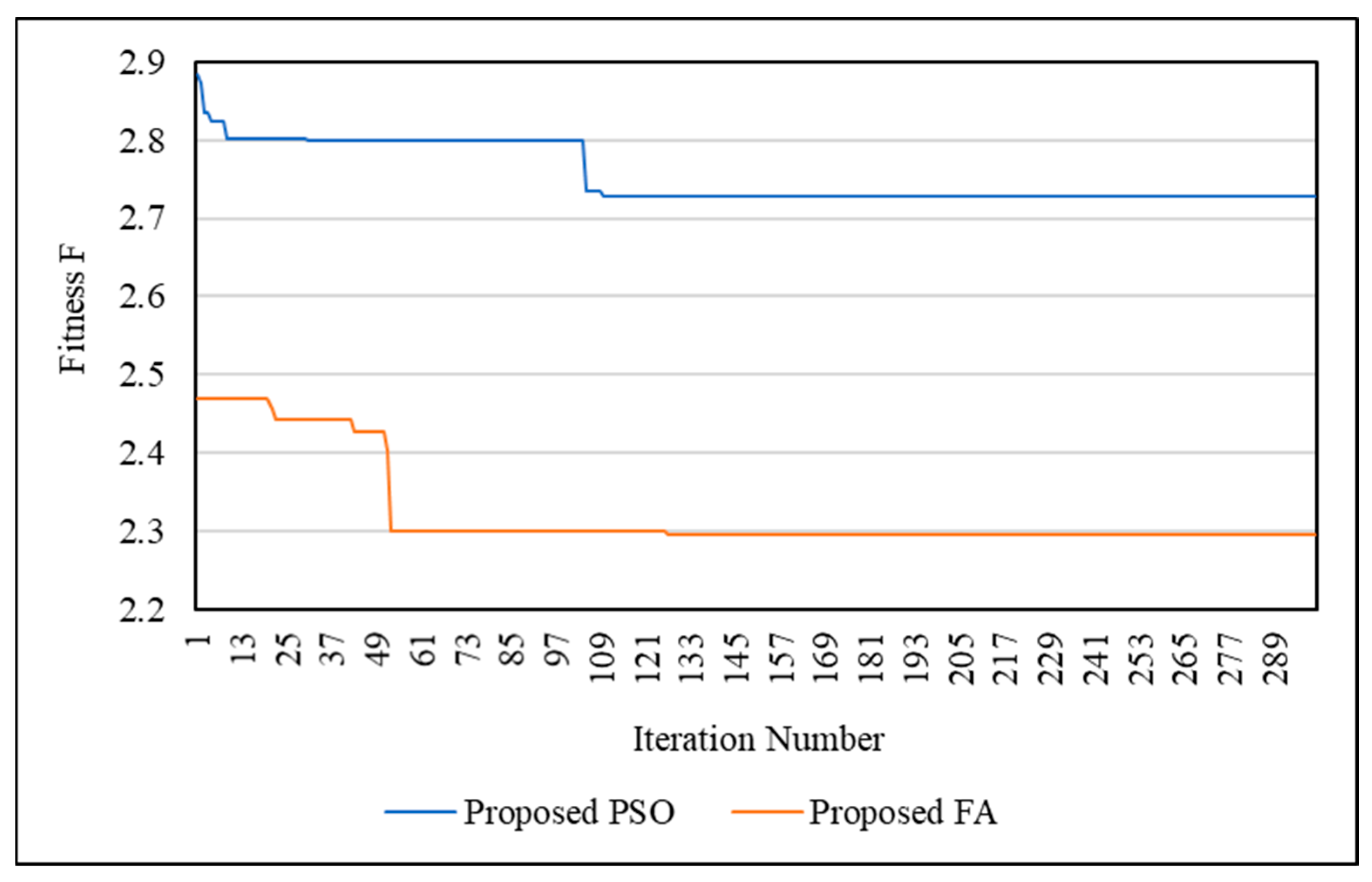
4.2.3. Impact of SSO on Optimization Performance
5. Conclusions
Author Contributions
Funding
Data Availability Statement
Acknowledgments
Conflicts of Interest
References
- Shayeghi, H.; Mahdavi, M. Studying the effect of losses coefficient on transmission expansion planning using decimal codification based GA. Planning 2009, 5, 6. [Google Scholar]
- Macedo, L.H.; Franco, J.F.; Mahdavi, M.; Romero, R. A contribution to the optimization of the reconfiguration problem in radial distribution systems. J. Control Autom. Electr. Syst. 2018, 29, 756–768. [Google Scholar] [CrossRef]
- Hosseini, H.; Jalilzadeh, S.; Nabaei, V.; Govar, G.Z.; Mahdavi, M. Enhancing deregulated distribution network reliability for minimizing penalty cost based on reconfiguration using BPSO. In Proceedings of the 2008 IEEE 2nd International Power and Energy Conference, Johor Bahru, Malaysia, 1–3 December 2008; IEEE: New York, NY, USA, 2008; pp. 983–987. [Google Scholar]
- Zheng, W.; Huang, W.; Hill, D.J.; Hou, Y. An adaptive distributionally robust model for three-phase distribution network reconfiguration. IEEE Trans. Smart Grid 2020, 12, 1224–1237. [Google Scholar] [CrossRef]
- Mahdavi, M.; Alhelou, H.H.; Hatziargyriou, N.D.; Al-Hinai, A. An efficient mathematical model for distribution system reconfiguration using AMPL. IEEE Access 2021, 9, 79961–79993. [Google Scholar] [CrossRef]
- Baran, M.E.; Wu, F.F. Network reconfiguration in distribution systems for loss reduction and load balancing. IEEE Trans. Power Deliv. 1989, 4, 1401–1407. [Google Scholar] [CrossRef]
- Gupta, N.; Swarnkar, A.; Niazi, K. Distribution network reconfiguration for power quality and reliability improvement using Genetic Algorithms. Int. J. Electr. Power Energy Syst. 2014, 54, 664–671. [Google Scholar] [CrossRef]
- Swarnkar, A.; Gupta, N.; Niazi, K.R. Adapted ant colony optimization for efficient reconfiguration of balanced and unbalanced distribution systems for loss minimization. Swarm Evol. Comput. 2011, 1, 129–137. [Google Scholar] [CrossRef]
- Hu, W.; Chen, Z.; Bak-Jensen, B.; Hu, Y. Fuzzy adaptive particle swarm optimisation for power loss minimisation in distribution systems using optimal load response. IET Gener. Transm. Distrib. 2014, 8, 1–10. [Google Scholar] [CrossRef]
- Tang, J.; Liu, G.; Pan, Q. A review on representative swarm intelligence algorithms for solving optimization problems: Applications and trends. IEEE/CAA J. Autom. Sin. 2021, 8, 1627–1643. [Google Scholar] [CrossRef]
- Goswami, S.K.; Basu, S.K. A new algorithm for the reconfiguration of distribution feeders for loss minimization. IEEE Trans. Power Deliv. 1992, 7, 1484–1491. [Google Scholar] [CrossRef]
- Gomes, F.V.; Carneiro, S.; Pereira, J.L.R.; Vinagre, M.P.; Garcia, P.A.N.; De Araujo, L.R. A new distribution system reconfiguration approach using optimum power flow and sensitivity analysis for loss reduction. IEEE Trans. Power Syst. 2006, 21, 1616–1623. [Google Scholar] [CrossRef]
- Duan, D.-L.; Ling, X.-D.; Wu, X.-Y.; Zhong, B. Reconfiguration of distribution network for loss reduction and reliability improvement based on an enhanced genetic algorithm. Int. J. Electr. Power Energy Syst. 2015, 64, 88–95. [Google Scholar] [CrossRef]
- Narimani, M.R.; Azizi Vahed, A.; Azizipanah-Abarghooee, R.; Javidsharifi, M. Enhanced gravitational search algorithm for multi-objective distribution feeder reconfiguration considering reliability, loss and operational cost. IET Gener. Transm. Distrib. 2014, 8, 55–69. [Google Scholar] [CrossRef]
- Shen, X.; Shahidehpour, M.; Zhu, S.; Han, Y.; Zheng, J. Multi-stage planning of active distribution networks considering the co-optimization of operation strategies. IEEE Trans. Smart Grid 2016, 9, 1425–1433. [Google Scholar] [CrossRef]
- Azizivahed, A.; Arefi, A.; Ghavidel, S.; Shafie-Khah, M.; Li, L.; Zhang, J.; Catalão, J.P. Energy management strategy in dynamic distribution network reconfiguration considering renewable energy resources and storage. IEEE Trans. Sustain. Energy 2019, 11, 662–673. [Google Scholar] [CrossRef]
- Wang, B.; Zhu, H.; Xu, H.; Bao, Y.; Di, H. Distribution network reconfiguration based on NoisyNet deep Q-learning network. IEEE Access 2021, 9, 90358–90365. [Google Scholar] [CrossRef]
- Fu, X.; Guo, Q.; Sun, H. Statistical machine learning model for stochastic optimal planning of distribution networks considering a dynamic correlation and dimension reduction. IEEE Trans. Smart Grid 2020, 11, 2904–2917. [Google Scholar] [CrossRef]
- Islam, M.R.; Lu, H.; Hossain, M.; Li, L. Mitigating unbalance using distributed network reconfiguration techniques in distributed power generation grids with services for electric vehicles: A review. J. Clean. Prod. 2019, 239, 117932. [Google Scholar] [CrossRef]
- Sultana, B.; Mustafa, M.; Sultana, U.; Bhatti, A.R. Review on reliability improvement and power loss reduction in distribution system via network reconfiguration. Renew. Sustain. Energy Rev. 2016, 66, 297–310. [Google Scholar] [CrossRef]
- Muhammad, M.A.; Mokhlis, H.; Naidu, K.; Amin, A.; Franco, J.F.; Othman, M. Distribution network planning enhancement via network reconfiguration and DG integration using dataset approach and water cycle algorithm. J. Mod. Power Syst. Clean Energy 2019, 8, 86–93. [Google Scholar] [CrossRef]
- Pujari, H.K.; Rudramoorthy, M. Grey wolf optimisation algorithm for solving distribution network reconfiguration considering distributed generators simultaneously. Int. J. Sustain. Energy 2022, 41, 2121–2149. [Google Scholar] [CrossRef]
- Hamida, I.B.; Salah, S.B.; Msahli, F.; Mimouni, M.F. Optimal network reconfiguration and renewable DG integration considering time sequence variation in load and DGs. Renew. Energy 2018, 121, 66–80. [Google Scholar] [CrossRef]
- Essallah, S.; Khedher, A. Optimization of distribution system operation by network reconfiguration and DG integration using MPSO algorithm. Renew. Energy Focus 2020, 34, 37–46. [Google Scholar] [CrossRef]
- Abd El-salam, M.F.; Beshr, E.; Eteiba, M.B. A new hybrid technique for minimizing power losses in a distribution system by optimal sizing and siting of distributed generators with network reconfiguration. Energies 2018, 11, 3351. [Google Scholar] [CrossRef]
- Rahim, M.N.A.; Mokhlis, H.; Bakar, A.H.A.; Rahman, M.T.; Badran, O.; Mansor, N.N. Protection coordination toward optimal network reconfiguration and DG sizing. IEEE Access 2019, 7, 163700–163718. [Google Scholar] [CrossRef]
- Fathi, R.; Tousi, B.; Galvani, S. Allocation of renewable resources with radial distribution network reconfiguration using improved salp swarm algorithm. Appl. Soft Comput. 2023, 132, 109828. [Google Scholar] [CrossRef]
- Swaminathan, D.; Rajagopalan, A. Optimized Network Reconfiguration with Integrated Generation Using Tangent Golden Flower Algorithm. Energies 2022, 15, 8158. [Google Scholar] [CrossRef]
- Sayed, M.M.; Mahdy, M.Y.; Abdel Aleem, S.H.; Youssef, H.K.; Boghdady, T.A. Simultaneous Distribution Network Reconfiguration and Optimal Allocation of Renewable-Based Distributed Generators and Shunt Capacitors under Uncertain Conditions. Energies 2022, 15, 2299. [Google Scholar] [CrossRef]
- Tang, J.; Chen, X.; Zhu, X.; Zhu, F. Dynamic reallocation model of multiple unmanned aerial vehicle tasks in emergent adjustment scenarios. IEEE Trans. Aerosp. Electron. Syst. 2022, 59, 1139–1155. [Google Scholar] [CrossRef]
- Liu, Y.; Gu, X. Skeleton-network reconfiguration based on topological characteristics of scale-free networks and discrete particle swarm optimization. IEEE Trans. Power Syst. 2007, 22, 1267–1274. [Google Scholar] [CrossRef]
- Zhang, X.; Fu, X.; Xue, Y.; Chang, X.; Bai, X. A review on basic theory and technology of agricultural energy internet. IET Renew. Power Gener. 2023. [Google Scholar] [CrossRef]
- Fu, X.; Zhou, Y. Collaborative optimization of PV greenhouses and clean energy systems in rural areas. IEEE Trans. Sustain. Energy 2022, 14, 642–656. [Google Scholar] [CrossRef]
- Zin, A.A.M.; Ferdavani, A.K.; Khairuddin, A.B.; Naeini, M.M. Reconfiguration of radial electrical distribution network through minimum-current circular-updating-mechanism method. IEEE Trans. Power Syst. 2011, 27, 968–974. [Google Scholar]
- Venkatesh, B.; Ranjan, R.; Gooi, H. Optimal reconfiguration of radial distribution systems to maximize loadability. IEEE Trans. Power Syst. 2004, 19, 260–266. [Google Scholar] [CrossRef]
- Tyagi, A.; Verma, A.; Bijwe, P. Reconfiguration for loadability limit enhancement of distribution systems. IET Gener. Transm. Distrib. 2018, 12, 88–93. [Google Scholar] [CrossRef]
- Aman, M.M.; Jasmon, G.B.; Bakar, A.H.A.; Mokhlis, H. Optimum network reconfiguration based on maximization of system loadability using continuation power flow theorem. Int. J. Electr. Power Energy Syst. 2014, 54, 123–133. [Google Scholar] [CrossRef]
- Aman, M.M.; Jasmon, G.B.; Bakar, A.H.A.; Mokhlis, H. A new approach for optimum simultaneous multi-DG distributed generation Units placement and sizing based on maximization of system loadability using HPSO (hybrid particle swarm optimization) algorithm. Energy 2014, 66, 202–215. [Google Scholar] [CrossRef]
- Latreche, Y.; Bouchekara, H.; Javaid, M.; Aman, M.; Mokhlis, H.; Kerrour, F. Optimal incorporation of multiple distributed generation units based on a new system maximum loadability computation approach and vortex searching algorithm. Int. J. Appl. Power Eng. (IJAPE) 2019, 8, 186–208. [Google Scholar] [CrossRef]
- Raut, U.; Mishra, S. An improved Elitist–Jaya algorithm for simultaneous network reconfiguration and DG allocation in power distribution systems. Renew. Energy Focus 2019, 30, 92–106. [Google Scholar] [CrossRef]
- Quadri, I.A.; Bhowmick, S.; Joshi, D. Multi-objective approach to maximise loadability of distribution networks by simultaneous reconfiguration and allocation of distributed energy resources. IET Gener. Transm. Distrib. 2018, 12, 5700–5712. [Google Scholar] [CrossRef]
- Hemmatpour, M.H.; Mohammadian, M.; Gharaveisi, A.A. Optimum islanded microgrid reconfiguration based on maximization of system loadability and minimization of power losses. Int. J. Electr. Power Energy Syst. 2016, 78, 343–355. [Google Scholar] [CrossRef]
- Abbasi, M. Simultaneous Power Network Reconfiguration and DG Allocation Using Improved Jaya Algorithm for Maximum Loadability Improvement and Power Loss Reduction. Comput. Res. Prog. Appl. Sci. Eng. 2021, 7, 2310. [Google Scholar]
- Bernardon, D.; Mello, A.; Pfitscher, L.; Canha, L.; Abaide, A.; Ferreira, A. Real-time reconfiguration of distribution network with distributed generation. Electr. Power Syst. Res. 2014, 107, 59–67. [Google Scholar] [CrossRef]
- Koutsoukis, N.C.; Siagkas, D.O.; Georgilakis, P.S.; Hatziargyriou, N.D. Online reconfiguration of active distribution networks for maximum integration of distributed generation. IEEE Trans. Autom. Sci. Eng. 2016, 14, 437–448. [Google Scholar] [CrossRef]
- Yin, Z.; Ji, X.; Zhang, Y.; Liu, Q.; Bai, X. Data-driven approach for real-time distribution network reconfiguration. IET Gener. Transm. Distrib. 2020, 14, 2450–2463. [Google Scholar] [CrossRef]
- Masteri, K.; Venkatesh, B. Real-time smart distribution system reconfiguration using complementarity. Electr. Power Syst. Res. 2016, 134, 97–104. [Google Scholar] [CrossRef]
- Shukla, J.; Das, B.; Pant, V. Consideration of small signal stability in multi-objective DS reconfiguration in the presence of distributed generation. IET Gener. Transm. Distrib. 2017, 11, 236–245. [Google Scholar] [CrossRef]
- Fetouh, T.; Elsayed, A.M. Optimal control and operation of fully automated distribution networks using improved tunicate swarm intelligent algorithm. IEEE Access 2020, 8, 129689–129708. [Google Scholar] [CrossRef]
- Xing, H.; Hong, S. Ordinal optimisation approach for complex distribution network reconfiguration. J. Eng. 2019, 2019, 5055–5058. [Google Scholar] [CrossRef]
- Venkaiah, C.; Jain, R.V. Multi-objective JAYA algorithm based optimal location and sizing of distributed generation in a radial distribution system. In Proceedings of the 2017 IEEE PES Asia-Pacific Power and Energy Engineering Conference (APPEEC), Bangalore, India, 8–10 November 2017; IEEE: New York, NY, USA, 2017; pp. 1–6. [Google Scholar]
- Saaty, R.W. The analytic hierarchy process—What it is and how it is used. Math. Model. 1987, 9, 161–176. [Google Scholar] [CrossRef]
- Wilson, B.M.R.; Khazaei, B.; Hirsch, L. Cloud adoption decision support for SMEs using Analytical Hierarchy Process (AHP). In Proceedings of the 2016 IEEE 4th Workshop on Advances in Information, Electronic and Electrical Engineering (AIEEE), Vilnius, Lithuania, 10–12 November 2016; IEEE: New York, NY, USA, 2016; pp. 1–4. [Google Scholar]
- Gandomi, A.H.; Yang, X.-S.; Alavi, A.H. Mixed variable structural optimization using firefly algorithm. Comput. Struct. 2011, 89, 2325–2336. [Google Scholar] [CrossRef]
- Yang, X. Nature-Inspired Metaheuristic Algorithms. 2010. Firefly Algorithm; Luniver Press: Bristol, UK, 2011; pp. 79–90. [Google Scholar]
- Liang, R.-H.; Wang, J.-C.; Chen, Y.-T.; Tseng, W.-T. An enhanced firefly algorithm to multi-objective optimal active/reactive power dispatch with uncertainties consideration. Int. J. Electr. Power Energy Syst. 2015, 64, 1088–1097. [Google Scholar] [CrossRef]
- Yang, X.-S. Firefly Algorithms for Multimodal Optimization, International Symposium on Stochastic Algorithms, 2009; Springer: Berlin/Heidelberg, Germany, 2009; pp. 169–178. [Google Scholar]
- Eberhart, R.; Kennedy, J. In A new optimizer using particle swarm theory, MHS’95. In Proceedings of the Sixth International Symposium on Micro Machine and Human Science, Nagoya, Japan, 4–6 October 1995; IEEE: New York, NY, USA, 1995; pp. 39–43. [Google Scholar]
- Balakrishna, G.; Babu, C.S. Particle swarm optimization based network reconfiguration in distribution system with distributed generation and capacitor placement. Int. J. Eng. Sci. 2014, 3, 55–60. [Google Scholar]
- Badran, O.; Mekhilef, S.; Mokhlis, H.; Dahalan, W. Optimal reconfiguration of distribution system connected with distributed generations: A review of different methodologies. Renew. Sustain. Energy Rev. 2017, 73, 854–867. [Google Scholar] [CrossRef]
- Bouchekara, H. Comprehensive Review of Radial Distribution Test Systems; Authorea: Hoboken, NJ, USA, 2020. [Google Scholar]
- Savier, J.; Das, D. Impact of network reconfiguration on loss allocation of radial distribution systems. IEEE Trans. Power Deliv. 2007, 22, 2473–2480. [Google Scholar] [CrossRef]
- Rao, R.S.; Ravindra, K.; Satish, K.; Narasimham, S. Power loss minimization in distribution system using network reconfiguration in the presence of distributed generation. IEEE Trans. Power Syst. 2012, 28, 317–325. [Google Scholar] [CrossRef]
- Imran, A.M.; Kowsalya, M.; Kothari, D. A novel integration technique for optimal network reconfiguration and distributed generation placement in power distribution networks. Int. J. Electr. Power Energy Syst. 2014, 63, 461–472. [Google Scholar] [CrossRef]
- Badran, O.; Mokhlis, H.; Mekhilef, S.; Dahalan, W. Multi-Objective network reconfiguration with optimal DG output using meta-heuristic search algorithms. Arab. J. Sci. Eng. 2018, 43, 2673–2686. [Google Scholar] [CrossRef]
- Haider, W.; Hassan, S.J.U.; Mehdi, A.; Hussain, A.; Adjayeng, G.O.M.; Kim, C.-H. Voltage profile enhancement and loss minimization using optimal placement and sizing of distributed generation in reconfigured network. Machines 2021, 9, 20. [Google Scholar] [CrossRef]
- Raut, U.; Mishra, S. An improved sine–cosine algorithm for simultaneous network reconfiguration and DG allocation in power distribution systems. Appl. Soft Comput. 2020, 92, 106293. [Google Scholar] [CrossRef]


| Criteria | Numeric Rating | Reciprocal (Decimal) |
|---|---|---|
| Equal importance | 1 | 1 |
| Moderate importance | 3 | 0.33333 |
| Strong importance | 5 | 0.2 |
| Very strong importance | 7 | 0.142857 |
| Criteria | Ploss | Qloss | MLC | IVD | Totals = ∑Each Row | Weight = Totals/Sum |
|---|---|---|---|---|---|---|
| Ploss | 1 | 3 | 5 | 7 | 16 | 0.493537634 |
| Qloss | 0.3333 | 1 | 3 | 5 | 9.3333 | 0.287895925 |
| MLC | 0.2 | 0.6 | 1 | 3 | 4.8 | 0.14806129 |
| IVD | 0.142857 | 0.42857 | 0.71428 | 1 | 2.285707 | 0.070505151 |
| Sum | 11.333 | 1 | ||||
| Optimization Technique | Initial Form | Proposed PSO | Proposed FA |
|---|---|---|---|
| Tie Switch | 33, 34, 35, 36, 37 | 27, 17, 6, 11, 13 | 27, 17, 6, 11, 13 |
| DG Location | ------- | 15, 8, 29 | 15, 7, 29 |
| DG Sizing (MW) | NO DG | 0.47608 | 0.44495 |
| 0.72063 | 0.66420 | ||
| 1.86442 | 1.73274 | ||
| Fitness | ------- | 0.3043 | 0.27798 |
| Load Active Power P (kW) | 3715 | 4264.2 | 3984.8 |
| Load Reactive Power Q (kVAR) | 2300 | 2553.5 | 2424.3 |
| Load Active Power Addition (%) | ------- | 14.78 | 7.26 |
| Load Reactive Power Addition (%) | ------- | 11.02 | 5.4 |
| Active Power Loss (kW) | 202.4 | 73.3 | 67.02 |
| Reactive Power Loss (kVAR) | 135 | 55.0 | 49.78 |
| Active Power Reduction (%) | ------- | 63.78 | 66.89 |
| Reactive Power Reduction (%) | ------- | 59.26 | 63.13 |
| Minimum Bus Voltage | 0.913 | 0.9663 | 0.9675 |
| Maximum Bus Voltage | 1 | 1 | 1 |
| Optimization Technique | Initial Form | Proposed PSO | Proposed FA |
|---|---|---|---|
| Tie Switch | 69, 70, 71, 72, 73 | 58, 39, 25, 18, 43 | 17, 42, 62, 56, 13 |
| DG Location | ------- | 63, 68, 37 | 3, 61, 21 |
| DG Sizing (MW) | NO DG | 1.806623 | 1.43198 |
| 1.049059 | 1.64518 | ||
| 0.576134 | 1.00133 | ||
| Fitness | ------- | 0.26666 | 0.20972 |
| Load Active Power P (kW) | 3801.89 | 3866.91 | 3849.42 |
| Load Reactive Power Q (kVAR) | 2694.1 | 2739.77 | 2727.53 |
| Load Active Power Addition (%) | ------- | 1.71 | 1.25 |
| Load Reactive Power Addition (%) | ------- | 1.695 | 1.24 |
| Active Power Loss (kW) | 224.557 | 57.88 | 46.093 |
| Reactive Power Loss (kVAR) | 102 | 47.348 | 36.553 |
| Active Power Reduction (%) | ------- | 74.22 | 79.47 |
| Reactive Power Reduction (%) | ------- | 53.58 | 64.16 |
| Minimum Bus Voltage | 0.9093 | 0.976022 | 0.984597 |
| Maximum Bus Voltage | 1 | 1.0026 | 1 |
| MLC Factor | Proposed PSO | Proposed FA | MLC Factor | Proposed PSO | Proposed FA |
|---|---|---|---|---|---|
| λ-1 | 1 | 1 | λ-18 | 1.26345 | 1.12366 |
| λ-2 | 1.11492 | 1.06474 | λ-19 | 1.26851 | 1.13568 |
| λ-3 | 1.28074 | 1.14458 | λ-20 | 1.26968 | 1.12472 |
| λ-4 | 1.03133 | 1.02749 | λ-21 | 1.22302 | 1.10562 |
| λ-5 | 1.05679 | 1.02962 | λ-22 | 1.25494 | 1.1231 |
| λ-6 | 1.15976 | 1.07315 | λ-23 | 1.11083 | 1.06036 |
| λ-7 | 1.06558 | 1.04158 | λ-24 | 1.16919 | 1.0942 |
| λ-8 | 1.21678 | 1.09916 | λ-25 | 1.09225 | 1.02418 |
| λ-9 | 1.25074 | 1.12805 | λ-26 | 1.26249 | 1.12886 |
| λ-10 | 1.21829 | 1.10385 | λ-27 | 1.32157 | 1.14432 |
| λ-11 | 1.01628 | 1.01871 | λ-28 | 1.15529 | 1.07592 |
| λ-12 | 1.28572 | 1.1169 | λ-29 | 1.10417 | 1.03353 |
| λ-13 | 1.09237 | 1.05092 | λ-30 | 1.00002 | 1.00001 |
| λ-14 | 1.0198 | 1.0103 | λ-31 | 1.18132 | 1.09869 |
| λ-15 | 1.23565 | 1.13678 | λ-32 | 1.10245 | 1.05436 |
| λ-16 | 1.04101 | 1.03011 | λ-33 | 1.2751 | 1.14309 |
| λ-17 | 1.19403 | 1.10891 |
| Bus Number | Initial Load | Proposed PSO | Proposed FA | Bus Number | Initial Load | Proposed PSO | Proposed FA |
|---|---|---|---|---|---|---|---|
| 1 | 0 | 0 | 0 | 18 | 90 | 113.71 | 101.13 |
| 2 | 100 | 111.49 | 106.47 | 19 | 90 | 114.17 | 102.21 |
| 3 | 90 | 115.27 | 103.01 | 20 | 90 | 114.27 | 101.22 |
| 4 | 120 | 123.76 | 123.3 | 21 | 90 | 110.07 | 99.51 |
| 5 | 60 | 63.41 | 61.78 | 22 | 90 | 112.94 | 101.08 |
| 6 | 60 | 69.59 | 64.39 | 23 | 90 | 99.97 | 95.43 |
| 7 | 200 | 213.12 | 208.32 | 24 | 420 | 491.06 | 459.56 |
| 8 | 200 | 243.36 | 219.83 | 25 | 420 | 458.75 | 430.16 |
| 9 | 60 | 75.04 | 67.68 | 26 | 60 | 75.75 | 67.73 |
| 10 | 60 | 73.1 | 66.23 | 27 | 60 | 79.29 | 68.66 |
| 11 | 45 | 45.73 | 45.84 | 28 | 60 | 69.32 | 64.56 |
| 12 | 60 | 77.14 | 67.01 | 29 | 120 | 132.5 | 124.02 |
| 13 | 60 | 65.54 | 63.06 | 30 | 200 | 200 | 200 |
| 14 | 120 | 122.38 | 121.24 | 31 | 150 | 177.2 | 164.8 |
| 15 | 60 | 74.14 | 68.21 | 32 | 210 | 231.51 | 221.42 |
| 16 | 60 | 62.46 | 61.81 | 33 | 60 | 76.51 | 68.59 |
| 17 | 60 | 71.64 | 66.53 |
| Bus Number | Initial Load | Proposed PSO | Proposed FA | Bus Number | Initial Load | Proposed PSO | Proposed FA |
|---|---|---|---|---|---|---|---|
| 1 | 0 | 0 | 0 | 18 | 40 | 50.54 | 44.95 |
| 2 | 60 | 66.9 | 63.88 | 19 | 40 | 50.74 | 45.43 |
| 3 | 40 | 51.23 | 45.78 | 20 | 40 | 50.79 | 44.99 |
| 4 | 80 | 82.51 | 82.2 | 21 | 40 | 48.92 | 44.22 |
| 5 | 30 | 31.7 | 30.89 | 22 | 40 | 50.2 | 44.92 |
| 6 | 20 | 23.2 | 21.46 | 23 | 50 | 55.54 | 53.02 |
| 7 | 100 | 106.56 | 104.16 | 24 | 200 | 233.84 | 218.84 |
| 8 | 100 | 121.68 | 109.92 | 25 | 200 | 218.45 | 204.84 |
| 9 | 20 | 25.01 | 22.56 | 26 | 25 | 31.56 | 28.22 |
| 10 | 20 | 24.37 | 22.08 | 27 | 25 | 33.04 | 28.61 |
| 11 | 30 | 30.49 | 30.56 | 28 | 20 | 23.11 | 21.52 |
| 12 | 35 | 45 | 39.09 | 29 | 70 | 77.29 | 72.35 |
| 13 | 35 | 38.23 | 36.78 | 30 | 600 | 600.01 | 600.01 |
| 14 | 80 | 81.58 | 80.82 | 31 | 70 | 82.69 | 76.91 |
| 15 | 10 | 12.36 | 11.37 | 32 | 100 | 110.25 | 105.44 |
| 16 | 20 | 20.82 | 20.6 | 33 | 40 | 51 | 45.72 |
| 17 | 20 | 23.88 | 22.18 |
| Maximum Load Capacity Factor | Proposed PSO | Proposed FA | Maximum Load Capacity Factor | Proposed PSO | Proposed FA |
|---|---|---|---|---|---|
| λ-1 | 1 | 1 | λ-36 | 1.025778 | 1.01425 |
| λ-2 | 1 | 1 | λ-37 | 1.038855 | 1.01915 |
| λ-3 | 1 | 1 | λ-38 | 1 | 1 |
| λ-4 | 1 | 1 | λ-39 | 1.022803 | 1.03341 |
| λ-5 | 1 | 1 | λ-40 | 1.026894 | 1.01272 |
| λ-6 | 1.005305 | 1.01705 | λ-41 | 1.019443 | 1.02073 |
| λ-7 | 1.03952 | 1.0494 | λ-42 | 1 | 1 |
| λ-8 | 1.028485 | 1.0289 | λ-43 | 1.001089 | 1.00514 |
| λ-9 | 1.032341 | 1.00456 | λ-44 | 1 | 1 |
| λ-10 | 1.003023 | 1.04573 | λ-45 | 1.042301 | 1.01149 |
| λ-11 | 1.030453 | 1.01513 | λ-46 | 1.007325 | 1.02505 |
| λ-12 | 1.031857 | 1.03553 | λ-47 | 1 | 1 |
| λ-13 | 1.0371 | 1.0382 | λ-48 | 1.027221 | 1.01893 |
| λ-14 | 1.030453 | 1.01902 | λ-49 | 1.005623 | 1.01091 |
| λ-15 | 1 | 1 | λ-50 | 1.01474 | 1.0022 |
| λ-16 | 1.047649 | 1.01935 | λ-51 | 1.04548 | 1.01761 |
| λ-17 | 1.034622 | 1.03188 | λ-52 | 1.049495 | 1.01915 |
| λ-18 | 1.044751 | 1.02186 | λ-53 | 1.03668 | 1.02785 |
| λ-19 | 1 | 1 | λ-54 | 1.037489 | 1.03834 |
| λ-20 | 1.022179 | 1.04649 | λ-55 | 1.016188 | 1.04728 |
| λ-21 | 1.032805 | 1.04264 | λ-56 | 1 | 1 |
| λ-22 | 1.018165 | 1.02273 | λ-57 | 1 | 1 |
| λ-23 | 1 | 1 | λ-58 | 1 | 1 |
| λ-24 | 1.000589 | 1.04537 | λ-59 | 1.011154 | 1.01558 |
| λ-25 | 1 | 1 | λ-60 | 1 | 1 |
| λ-26 | 1.024762 | 1.03636 | λ-61 | 1.005182 | 1.00089 |
| λ-27 | 1.022704 | 1.02011 | λ-62 | 1.031962 | 1.00698 |
| λ-28 | 1.035366 | 1.03257 | λ-63 | 1 | 1 |
| λ-29 | 1.002183 | 1.00179 | λ-64 | 1.026842 | 1.00715 |
| λ-30 | 1 | 1 | λ-65 | 1.026854 | 1.02157 |
| λ-31 | 1 | 1 | λ-66 | 1.02008 | 1.00831 |
| λ-32 | 1 | 1 | λ-67 | 1.027917 | 1.01231 |
| λ-33 | 1.029619 | 1.04497 | λ-68 | 1.007607 | 1.04584 |
| λ-34 | 1.029734 | 1.02319 | λ-69 | 1.046024 | 1.00753 |
| λ-35 | 1.028754 | 1.04176 |
| Bus Number | Initial Load | Proposed PSO | Proposed FA | Bus Number | Initial Load | Proposed PSO | Proposed FA |
|---|---|---|---|---|---|---|---|
| 1 | 0 | 0 | 0 | 36 | 26 | 26.67 | 26.37 |
| 2 | 0 | 0 | 0 | 37 | 26 | 27.01 | 26.5 |
| 3 | 0 | 0 | 0 | 38 | 0 | 0 | 0 |
| 4 | 0 | 0 | 0 | 39 | 24 | 24.55 | 24.8 |
| 5 | 0 | 0 | 0 | 40 | 24 | 24.65 | 24.31 |
| 6 | 2.6 | 2.61 | 2.64 | 41 | 1.2 | 1.22 | 1.22 |
| 7 | 40.4 | 42 | 42.4 | 42 | 0 | 0 | 0 |
| 8 | 75 | 77.14 | 77.17 | 43 | 6 | 6.01 | 6.03 |
| 9 | 30 | 30.97 | 30.14 | 44 | 0 | 0 | 0 |
| 10 | 28 | 28.08 | 29.28 | 45 | 39.22 | 40.88 | 39.67 |
| 11 | 145 | 149.42 | 147.19 | 46 | 39.22 | 39.51 | 40.2 |
| 12 | 145 | 149.62 | 150.15 | 47 | 0 | 0 | 0 |
| 13 | 8 | 8.3 | 8.31 | 48 | 79 | 81.15 | 80.5 |
| 14 | 8 | 8.24 | 8.15 | 49 | 384.7 | 386.86 | 388.9 |
| 15 | 0 | 0 | 0 | 50 | 384.7 | 390.37 | 385.55 |
| 16 | 45.5 | 47.67 | 46.38 | 51 | 40.5 | 42.34 | 41.21 |
| 17 | 60 | 62.08 | 61.91 | 52 | 3.6 | 3.78 | 3.67 |
| 18 | 60 | 62.69 | 61.31 | 53 | 4.35 | 4.51 | 4.47 |
| 19 | 0 | 0 | 0 | 54 | 26.4 | 27.39 | 27.41 |
| 20 | 1 | 1.02 | 1.05 | 55 | 24 | 24.39 | 25.13 |
| 21 | 114 | 117.74 | 118.86 | 56 | 0 | 0 | 0 |
| 22 | 5 | 5.09 | 5.11 | 57 | 0 | 0 | 0 |
| 23 | 0 | 0 | 0 | 58 | 0 | 0 | 0 |
| 24 | 28 | 28.02 | 29.27 | 59 | 100 | 101.12 | 101.56 |
| 25 | 0 | 0 | 0 | 60 | 0 | 0 | 0 |
| 26 | 14 | 14.35 | 14.51 | 61 | 1244 | 1250.45 | 1245.11 |
| 27 | 14 | 14.32 | 14.28 | 62 | 32 | 33.02 | 32.22 |
| 28 | 26 | 26.92 | 26.85 | 63 | 0 | 0 | 0 |
| 29 | 26 | 26.06 | 26.05 | 64 | 227 | 233.09 | 228.62 |
| 30 | 0 | 0 | 0 | 65 | 59 | 60.58 | 60.27 |
| 31 | 0 | 0 | 0 | 66 | 18 | 18.36 | 18.15 |
| 32 | 0 | 0 | 0 | 67 | 18 | 18.5 | 18.22 |
| 33 | 14 | 14.41 | 14.63 | 68 | 28 | 28.21 | 29.28 |
| 34 | 19.5 | 20.08 | 19.95 | 69 | 28 | 29.29 | 28.21 |
| 35 | 6 | 6.17 | 6.25 |
| Bus Number | Initial Load | Proposed PSO | Proposed FA | Bus Number | Initial Load | Proposed PSO | Proposed FA |
|---|---|---|---|---|---|---|---|
| 1 | 0 | 0 | 0 | 36 | 18.55 | 19.03 | 18.81 |
| 2 | 0 | 0 | 0 | 37 | 18.55 | 19.27 | 18.91 |
| 3 | 0 | 0 | 0 | 38 | 0 | 0 | 0 |
| 4 | 0 | 0 | 0 | 39 | 17 | 17.39 | 17.57 |
| 5 | 0 | 0 | 0 | 40 | 17 | 17.46 | 17.22 |
| 6 | 2.2 | 2.21 | 2.24 | 41 | 1 | 1.02 | 1.02 |
| 7 | 30 | 31.19 | 31.48 | 42 | 0 | 0 | 0 |
| 8 | 54 | 55.54 | 55.56 | 43 | 4.3 | 4.3 | 4.32 |
| 9 | 22 | 22.71 | 22.1 | 44 | 0 | 0 | 0 |
| 10 | 19 | 19.06 | 19.87 | 45 | 26.3 | 27.41 | 26.6 |
| 11 | 104 | 107.17 | 105.57 | 46 | 26.3 | 26.49 | 26.96 |
| 12 | 104 | 107.31 | 107.7 | 47 | 0 | 0 | 0 |
| 13 | 5 | 5.19 | 5.19 | 48 | 56.4 | 57.94 | 57.47 |
| 14 | 5.5 | 5.67 | 5.6 | 49 | 274.5 | 276.04 | 277.49 |
| 15 | 0 | 0 | 0 | 50 | 274.5 | 278.55 | 275.1 |
| 16 | 30 | 31.43 | 30.58 | 51 | 28.3 | 29.59 | 28.8 |
| 17 | 35 | 36.21 | 36.12 | 52 | 2.7 | 2.83 | 2.75 |
| 18 | 35 | 36.57 | 35.77 | 53 | 3.5 | 3.63 | 3.6 |
| 19 | 0 | 0 | 0 | 54 | 19 | 19.71 | 19.73 |
| 20 | 0.6 | 0.61 | 0.63 | 55 | 17.2 | 17.48 | 18.01 |
| 21 | 81 | 83.66 | 84.45 | 56 | 0 | 0 | 0 |
| 22 | 3.5 | 3.56 | 3.58 | 57 | 0 | 0 | 0 |
| 23 | 0 | 0 | 0 | 58 | 0 | 0 | 0 |
| 24 | 20 | 20.01 | 20.91 | 59 | 72 | 72.8 | 73.12 |
| 25 | 0 | 0 | 0 | 60 | 0 | 0 | 0 |
| 26 | 10 | 10.25 | 10.36 | 61 | 888 | 892.6 | 888.79 |
| 27 | 10 | 10.23 | 10.2 | 62 | 23 | 23.74 | 23.16 |
| 28 | 18.6 | 19.26 | 19.21 | 63 | 0 | 0 | 0 |
| 29 | 18.6 | 18.64 | 18.63 | 64 | 162 | 166.35 | 163.16 |
| 30 | 0 | 0 | 0 | 65 | 42 | 43.13 | 42.91 |
| 31 | 0 | 0 | 0 | 66 | 13 | 13.26 | 13.11 |
| 32 | 0 | 0 | 0 | 67 | 13 | 13.36 | 13.16 |
| 33 | 10 | 10.3 | 10.45 | 68 | 20 | 20.15 | 20.92 |
| 34 | 14 | 14.42 | 14.32 | 69 | 20 | 20.92 | 20.15 |
| 35 | 4 | 4.12 | 4.17 |
| Simultaneous DNR and DG-LS | Tie Switch | DG’s Output (MW) | Minimum Voltage Bus (p.u) | Ploss (kW) | Reduction Loss (%) |
|---|---|---|---|---|---|
| GA [63] | 7, 28, 32, 34, 10 | 1.96330 | 0.9766 | 75.13 | 62.920 |
| RGA [63] | 7, 12, 27, 32, 9 | 1.774 | 0.9691 | 74.32 | 63.330 |
| HSA [63] | 7, 14, 28, 32, 10 | 1.66840 | 0.9700 | 73.05 | 63.950 |
| FWA [64] | 7, 14, 28, 32, 11 | 1.68410 | 0.9713 | 67.110 | 66.890 |
| EP [65] | 7, 9, 28, 32, 8 | 1.96380 | 0.9710 | 73.9710 | 63.490 |
| PSO [65] | 7, 13, 28, 32, 10 | 1.7660 | 0.97380 | 72.4210 | 64.3 |
| GSA [65] | 7, 13, 28, 32, 9 | 1.7450 | 0.97420 | 72.4250 | 64.250 |
| FA [65] | 7, 13, 28, 32, 10 | 1.8250 | 0.975 | 72.3610 | 64.280 |
| PSO [66] | 7, 14, 28, 32, 9 | 2.95410 | 0.96110 | 64.910 | 67.960 |
| MPSO [24] | 7,14, 32, 37, 9 | 1.09230 | 0.97640 | 62.40 | 68.320 |
| ISCA [67] | 7, 14, 28, 31, 9 | 1.69120 | - | 66.810 | 67.030 |
| The Proposed Method by FA | 34, 28, 11, 32, 33 | 2.56011 | 0.969724 | 54.997 | 72.83 |
| Simultaneous DNR and DG-LS | Tie Switch | DG’s Output (MW) | Minimum Voltage Bus (p.u) | Ploss (kW) | Reduction Loss (%) |
|---|---|---|---|---|---|
| GA [63] | 10, 45, 55, 62, 15 | 2.02920 | 0.97270 | 46.5 | 73.380 |
| RGA [63] | 10, 14, 55, 62, 16 | 2.06540 | 0.97420 | 44.230 | 80.320 |
| HSA [63] | 69, 13, 58, 61, 17 | 1.87180 | 0.97360 | 40.3 | 82.080 |
| FWA [64] | 69, 70, 13, 55, 63 | 1.8182 | 0.9796 | 39.25 | 82.55 |
| MPSO [24] | 14, 58, 61, 69, 70 | 2.2736 | 0.98994 | 42.2 | 81.1 |
| ISCA [67] | 12, 9, 57, 63, 69 | 1.8731 | - | 39.73 | 82.34 |
| The Proposed Method by FA | 13, 12, 62, 10, 57 | 2.4012 | 0.98035 | 39.16 | 82.56 |
| Optimization Technique | Step No. | SSO | Voltage Bus (p.u) (at Bus) | Fitness (F) | Ploss (kW) | Qloss (kVAR) | Total Ploss (kW) | Total Qloss (kVAR) | |
|---|---|---|---|---|---|---|---|---|---|
| Min | Max | ||||||||
| PSO | 1 | SW 37 Close | 0.9669 (18) | 1 (1) | 3.146 | 69.26 | 47.23 | 712.62 | 518.7 |
| 2 | SW 27 Open | 0.9675 (18) | 1 (1) | 76.91 | 54.08 | ||||
| 3 | SW 35 Close | 0.9718 (33) | 1 (1) | 70.18 | 51.09 | ||||
| 4 | SW 11 Open | 0.9721 (33) | 1 (1) | 70.22 | 51.41 | ||||
| 5 | SW 36 Close | 0.9717 (33) | 1 (1) | 66.58 | 49.82 | ||||
| 6 | SW 17 Open | 0.966 (18) | 1 (1) | 71.92 | 51.72 | ||||
| 7 | SW 33 Close | 0.966 (18) | 1 (1) | 70.84 | 51.51 | ||||
| 8 | SW 6 Open | 0.9663 (18) | 1 (1) | 71.77 | 53.47 | ||||
| 9 | SW 34 Close | 0.9663 (18) | 1 (1) | 71.63 | 53.34 | ||||
| 10 | SW 13 Open | 0.9663 (18) | 1 (1) | 73.31 | 55.03 | ||||
| FA | 1 | SW 37 Close | 0.9656 (18) | 1 (1) | 2.876 | 63.73 | 42.92 | 651.81 | 470.45 |
| 2 | SW 27 Open | 0.9663 (18) | 1 (1) | 70.74 | 49.19 | ||||
| 3 | SW 35 Close | 0.9725 (33) | 1 (1) | 64.19 | 46.48 | ||||
| 4 | SW 11 Open | 0.9726 (33) | 1 (1) | 63.99 | 46.46 | ||||
| 5 | SW 36 Close | 0.9728 (33) | 1 (1) | 60.59 | 45.06 | ||||
| 6 | SW 17 Open | 0.9672 (18) | 1 (1) | 65.59 | 46.87 | ||||
| 7 | SW 33 Close | 0.9674 (18) | 1 (1) | 64.62 | 46.84 | ||||
| 8 | SW 6 Open | 0.9675 (18) | 1 (1) | 65.73 | 48.48 | ||||
| 9 | SW 34 Close | 0.9675 (18) | 1 (1) | 65.61 | 48.37 | ||||
| 10 | SW 13 Open | 0.9675 (18) | 1 (1) | 67.02 | 49.78 | ||||
| Optimization Technique | Step No. | SSO | Voltage Bus (p.u) (at Bus) | Fitness (F) | Ploss (kW) | Qloss (kVAR) | Total Ploss (kW) | Total Qloss (kVAR) | |
|---|---|---|---|---|---|---|---|---|---|
| Min | Max | ||||||||
| PSO | 1 | SW 72 Close | 0.9855 (27) | 1.0019 (68) | 2.727 | 52.5 | 35.14 | 551.36 | 444.48 |
| 2 | SW 58 Open | 0.9778 (65) | 1.0041 (68) | 57.48 | 46.18 | ||||
| 3 | SW 70 Close | 0.9778 (65) | 1.0042 (68) | 54.76 | 45.49 | ||||
| 4 | SW 18 Open | 0.9778 (65) | 1.0042 (68) | 55.01 | 45.46 | ||||
| 5 | SW 73 Close | 0.984 (60) | 1.0009 (68) | 52 | 38.41 | ||||
| 6 | SW 25 Open | 0.976 (26) | 1.0048 (68) | 55.81 | 46.5 | ||||
| 7 | SW 71 Close | 0.976 (26) | 1.0056 (68) | 53.37 | 46 | ||||
| 8 | SW 43 Open | 0.976 (26) | 1.0031 (68) | 57.53 | 47.15 | ||||
| 9 | SW 69 Close | 0.976 (26) | 1.0033 (68) | 55.02 | 46.8 | ||||
| 10 | SW 39 Open | 0.976 (26) | 1.0026 (68) | 57.88 | 47.35 | ||||
| FA | 1 | SW 72 Close | 0.9809 (65) | 1.0134 (21) | 2.296 | 53.81 | 35.4 | 466.54 | 370.62 |
| 2 | SW 56 Open | 0.972 (65) | 1.0158 (21) | 58.66 | 46.75 | ||||
| 3 | SW 73 Close | 0.9854 (59) | 1 (1) | 51.01 | 38.08 | ||||
| 4 | SW 62 Open | 0.9846 (62) | 1 (1) | 50.43 | 36.96 | ||||
| 5 | SW 71 Close | 0.9846 (62) | 1 (1) | 41.28 | 35.04 | ||||
| 6 | SW 13 Open | 0.9846 (62) | 1.0004 (21) | 43.88 | 37.26 | ||||
| 7 | SW 70 Close | 0.9846 (62) | 1 (1) | 38.25 | 33.85 | ||||
| 8 | SW 17 Open | 0.9846 (62) | 1 (1) | 42.79 | 35.38 | ||||
| 9 | SW 69 Close | 0.9846 (62) | 1 (1) | 40.34 | 35.35 | ||||
| 10 | SW 42 Open | 0.9846 (62) | 1 (1) | 46.09 | 36.55 | ||||
Disclaimer/Publisher’s Note: The statements, opinions and data contained in all publications are solely those of the individual author(s) and contributor(s) and not of MDPI and/or the editor(s). MDPI and/or the editor(s) disclaim responsibility for any injury to people or property resulting from any ideas, methods, instructions or products referred to in the content. |
© 2023 by the authors. Licensee MDPI, Basel, Switzerland. This article is an open access article distributed under the terms and conditions of the Creative Commons Attribution (CC BY) license (https://creativecommons.org/licenses/by/4.0/).
Share and Cite
Badran, O.; Jallad, J. Multi-Objective Decision Approach for Optimal Real-Time Switching Sequence of Network Reconfiguration Realizing Maximum Load Capacity. Energies 2023, 16, 6779. https://doi.org/10.3390/en16196779
Badran O, Jallad J. Multi-Objective Decision Approach for Optimal Real-Time Switching Sequence of Network Reconfiguration Realizing Maximum Load Capacity. Energies. 2023; 16(19):6779. https://doi.org/10.3390/en16196779
Chicago/Turabian StyleBadran, Ola, and Jafar Jallad. 2023. "Multi-Objective Decision Approach for Optimal Real-Time Switching Sequence of Network Reconfiguration Realizing Maximum Load Capacity" Energies 16, no. 19: 6779. https://doi.org/10.3390/en16196779