Effect of Magnetic Shunts on Shell-Type Transformers Characteristics

Abstract

A three-dimensional analysis of the leakage magnetic field in a transformer with beveled edges in a magnetic shunt is described. This paper contains a mathematical description of the finite element method used in performing numerical calculations. Formulas allowing to determine the differential and integral parameters of the magnetic field were presented. Magnetic flux density distributions and the points with high values were determined in the shell-type core and movable shunt sub-areas. For different positions of the magnetic shunt, the short-circuit transformer reactance was calculated as the integral parameter of the above-mentioned magnetic field analysis. Their amounts for the extreme positions of the shunt were given, as well. The movable magnetic shunt geometry impact on the short-circuit current value is given. In order to validate the calculation results, the research included some point measurements of magnetic flux density vectors and the winding reactances as well, and good compliance with the simulation data has been obtained. Thus, this analysis can also be applied to other objects with movable shunts in their magnetic systems.

1. Introduction

1.1. Introduction

In the era of electronic static converters used in both low and high-voltage electric networks, many harmonics related to current and voltage distortions have appeared in the power net, which should be eliminated as much as possible. Therefore, one should use methods of changing voltage and current parameters without digitizing their waveforms. First, the systems operating with sinusoidal waves of the main electrical quantities should be introduced in designing. Among them are regulating transformers (RT) that adjust the external characteristics to specific loading requirements. Such structures can be called “natural” and apply to rectifier systems for charging energy sources (batteries) and supplying an electric arc. Due to the above, such special transformers (RT) operation enables obtaining the demanded operating characteristics [1,2,3]. For example, we need high leakage reactance (HLR) transformers that supply the electric arc [4]. Their characteristics are as well as those for the devices that operate close to short-circuit state [5]. Field analysis is needed to obtain the demanded characteristics or optimize their constructions [6,7].

Knowledge of the magnetic field distribution allows for determining the transformer key parameters without the need to build expensive prototypes or perform time-consuming and highly approximate analytical calculations [8,9]. In addition, knowledge of the magnetic flux density vector values at individual points in the area surrounding the core and windings makes it possible to determine the windings leakage reactance for different configurations of the core and windings arrangement [10]. In addition, it is possible to determine the impact of changes in these configurations on the transformer parameters. The results obtained through analytical calculations are often malformed with a large error, primarily due to the need for significant simplifications of the object’s physical geometry. The use of many correction factors requires knowledge of the approximate flux distribution, which is not always possible due to the complexity of the tested object structure [11].

The finite element method used in the calculations performed in this paper can be successfully adapted not only to electromagnetic field distribution but also to thermal [12], mechanical simulations [13,14,15], or transformer loss determination [16,17]. In addition, good compatibility is obtained not only for transformers but also for other objects, e.g., inductive sensors [18].

1.2. Historical Outline of Calculations of Hlr Transformers with Movable Magnetic Shunts

The variety of regulating transformers’ (RT) construction [5] makes it difficult to classify them. This also applies to high leakage reactance transformers (HLR) with shunt regulation of their current intensities. Therefore, the most general division seems to be in terms of the main leakage flux direction in relation to the windings axes. As a result of many analyses of the magnetic field in these transformers, B. Tomczuk proposed such a division in his Ph.D. [19]. They were divided into transformers with axial (yoke) leakage and those with radial ones.

Calculations for high leakage reactance transformers (HLR) with extreme magnetic shunt positions were performed repeatedly. For the transformer with yoke leakage, the superposition method of 2D magnetic field solutions was given in [19], which was published later [20]. In addition, for these transformers, but without a shunt, the method of integral equations developed by B. Tomczuk was also used [21,22].

Knowledge of leakage inductance is a particularly important parameter for transformer designers since it has a principal effect on the transformer’s short-circuit voltage. For objects with adjustable magnetic shunt positions, the use of 2D numerical computational methods is insufficient and can only be used at extreme magnetic shunt positions, due to the object asymmetry. The novelty of the presented work is to carry out a 3D analysis of the magnetic field distribution considering intermediate states of the magnetic shunt position and its different geometries. The results of 3D magnetic field analyses for many fixes of the transformer shunt were presented by the authors of this paper but only for a transformer with yoke dispersion.

2. Three-Dimensional Mathematical Modeling of Magnetic Flux Distribution in Radial Dispersion HLR Transformer

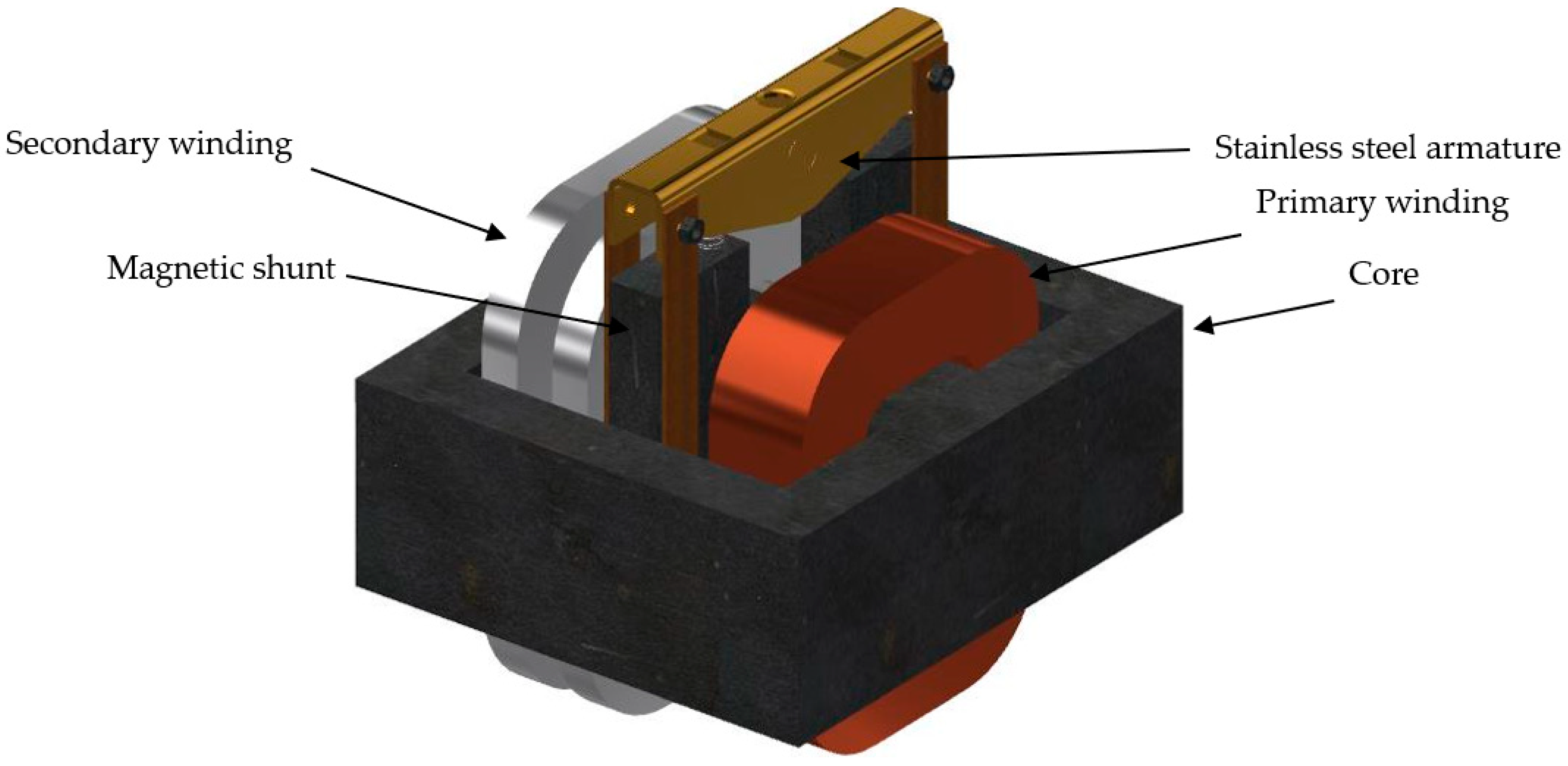
2.1. The Object under Consideration

In the present work, the authors describe three-dimensional magnetic field modeling in an HLR transformer with radial leakage field dissipation (Figure 1) and beveled edges in its magnetic shunt. The movable shunt packages are fastened with an armature made of stainless steel structural elements (Figure 1). Due to this, within our field analysis, we considered the magnetic system of the shell-type core and only shunt packages without non-magnetic structural components as well as the two windings made of different materials. The primary winding is made from a copper profile wire of rectangular cross-section (1.6 mm × 5 mm) and the secondary one is a two-section made of aluminum strip of cross-section (2.5 mm × 17 mm).

The transformer’s primary and secondary windings turn numbers equal 180 and 34, respectively. The transformer magnetic circuit with dimensions of 213 mm × 240 mm × 100 mm is a shell-type core structure [23].

Table 1. Parameters of the analyzed transformer.

Parameter	Value
Rated voltage	400 [V]
Maximum primary winding current	41 [A]
Maximum secondary winding current	225 [A]
Power	16 [kVA]

presents the rated parameters of the studied object.

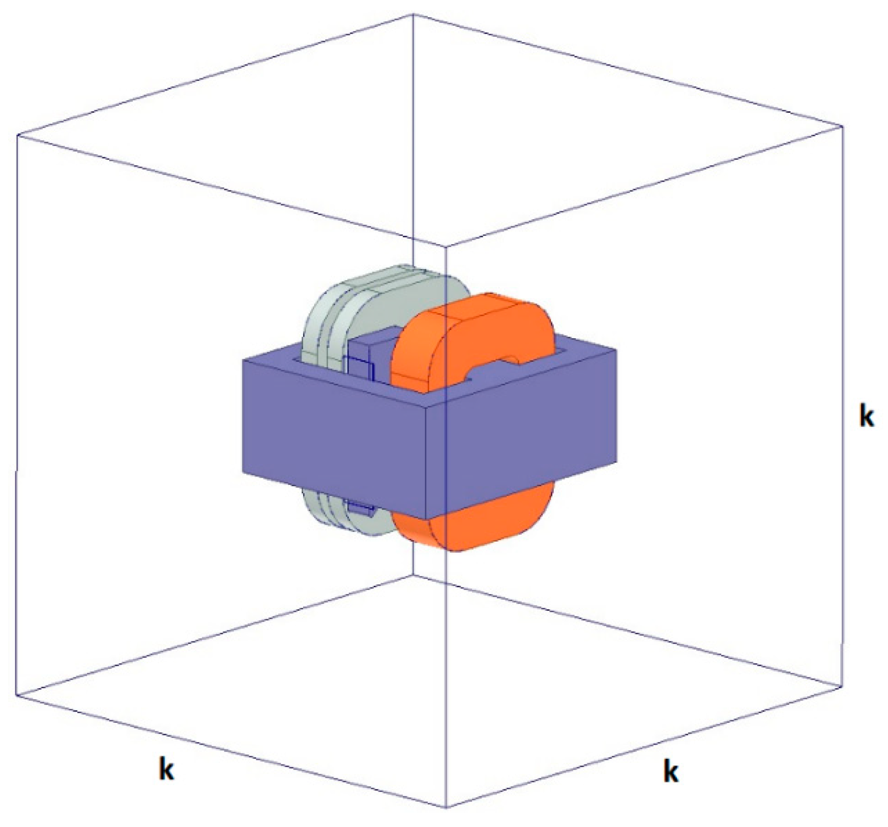
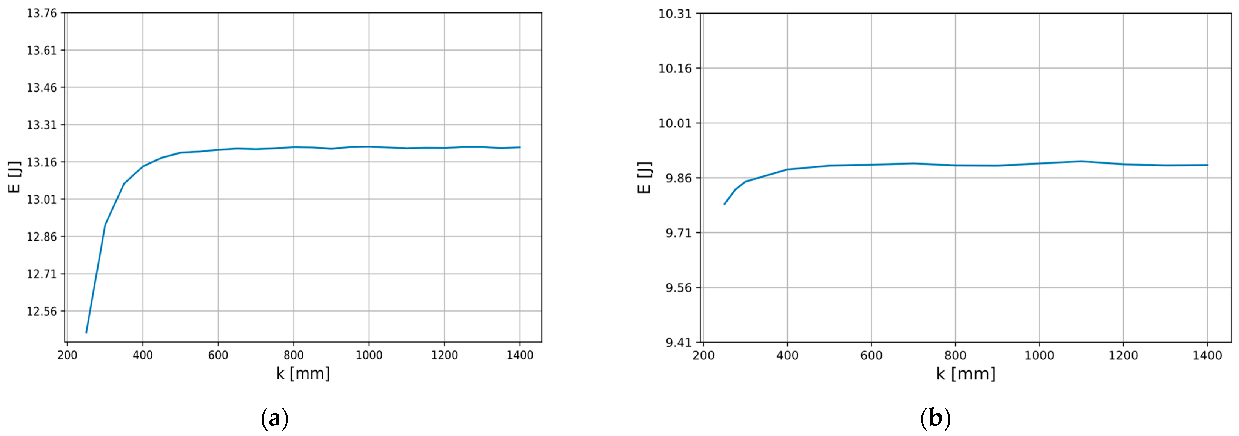
2.2. The Analysed Magnetic Field Area and Its Boundary Conditions

Due to the variable nature of the magnetic field distribution depending on the extraction of the shunt in relation to the transformer core, the mathematical model considers the appropriate adjustment of the analyzed area (Figure 2). The movable shunt providing a variable magnetic coupling between the primary and secondary windings in the object above allows for step-less regulation of the secondary voltage to maintain a secondary current.

For systems with a highly spatial distribution of the leakage fluxes, it is necessary to conduct a three-dimensional (3D) analysis of the unbounded magnetic field, which is the principal goal of this work. One of the most frequently used and well-programmed numerical methods is finite element one (FEM). Thus, this method has been used in this work. The magnetic potentials and flux distribution calculations were performed using FEM, applied in the commercial ANSYS Maxwell 2022 R1 software [24].

Our numerical calculations of the magnetic field distribution take place in a finite and defined by the boundary conditions space. The limitation of the computational region Ω is implemented by the Dirichlet and Neuman conditions. In the Dirichlet condition, the solution function takes known values on the edges of its domain, as in Equation (1) [25,26].

$$\mathrm{u}\left(\mathrm{P}\right)=\mathrm{g}\left(\mathrm{P}\right)\mathrm{for}\mathrm{P}\in \mathrm{S}$$

(1)

where:

• u(P)—the function sought at points inside the region Ω;
• g(P)—specified function for points P belonging to the S edge of the Ω area.

In the case of the Neumann boundary condition, the normal derivative on the S edge of the region takes known values, Equation (2) [25,26].

$$\frac{\partial \mathrm{u}}{\partial \mathrm{n}}\left(\mathrm{P}\right)=\mathrm{g}\left(\mathrm{P}\right)\mathrm{for}\mathrm{P}\in \mathrm{S}$$

(2)

The HLR transformers with increased leakage reactance, depending on the magnetic system structure and position of the movable shunt, can be characterized by an extensive magnetic field. The analysis of the computational area can be limited to the two extreme magnetic shunt positions, fully retracted and extended. In the case of a fully retracted shunt, the magnetic flux closes through the core-shunt gaps, so the magnetic flux density values outside the transformer window will be relatively small compared to those contained in the transformer window.

For the field analysis, we assumed a cubic computing space in which the transformer is located. Figure 2 shows the object under consideration, placed in the center of the cube area space of the “k” edge length. Therefore, before performing the proper field calculations, the influence of the cube’s edge length on the total energy accumulated in the leakage zone was analyzed (Figure 3). Although the transformer shell-type structure analyzed in this article characterizes relatively small leakage flux density values outside the transformer window, their influence on the leakage reactance must be considered.

Figure 3a shows that the increase in the calculation cube edge length above 0.6 m does not translate into a significant increase in the energy values of the outer air zone while causing a rise in the magnetic field analysis time. Based on Figure 3b, one can see that for the fully inserted magnetic shunt, the leakage energy outside the core has stabilized for the computational cube of a smaller edge value of 0.45 m. In conclusion, for the transformer without the magnetic shunt, a part of the magnetic field lines goes outside the transformer window, which requires consideration of a higher expanse. To increase the certainty of the correctness of the simulations, in further calculations described in this paper, the length of the edge of the computational area cube was assumed to be 1 m, regardless of the location of the magnetic shunt.

Symmetry and antisymmetry planes make it possible to reduce the computational area and thus reduce the number of discretization grid elements, which significantly reduces the size of the equations necessary to solve and the calculation time while maintaining the solution’s accuracy. Due to the movable magnetic shunt position and the object’s unsymmetrical winding execution, it is possible to include only one symmetry plane in the analysis, as in Figure 4. The conditions of symmetry and antisymmetry can be described by vector potential identities on both sides of these planes using Equations (3) and (4), respectively [25,26].

$${\mathrm{A}}_{1\left(\mathrm{x}2,\mathrm{y}2,\mathrm{z}2\right)}={{\mathrm{A}}^{\prime }}_{1\left(\mathrm{x}2,\mathrm{y}2,-\mathrm{z}2\right)}$$

(3)

$${\mathrm{A}}_{2\left(\mathrm{x}2,\mathrm{y}2,\mathrm{z}2\right)}={{\mathrm{A}}^{\prime }}_{2\left(\mathrm{x}2,\mathrm{y}2,-\mathrm{z}2\right)}$$

(4)

In transformers with adjustable magnetic shunt position, the area requiring special attention during discretization is the core-shunt gap, which is characterized by a high magnetic field variation; therefore, at least two mesh layers were forced in this area, and the maximum tetrahedron edge length did not exceed 2 mm. During the analysis, current excitation was used, and the non-linear magnetization characteristics of the transformer core sheets were considered, as in Figure 5.

The magnetic shunts used to regulate the current can be in cuboidal or tetrahedral shapes. For the shell-type transformer structure, the chamfering (beveling) magnetic shunt (Figure 6a) allows smooth current regulation in the secondary winding. The advantage of this shape is to increase the current regulation linearity by pulling out the magnetic shunt relative to the transformer window at the expense of hotspots in the corners of the core and shunt, which causes construction heating. Significantly increasing the beveling affects the maximum adjustment of the leakage reactance range. The paper examines the influence of the shunt chamfering on the transformer leakage reactance for different positions, with a constant of both primary and secondary ampere-turns windings, equal to θ = 1800 A. The simulation was performed by considering the transformer symmetry. Angle α was changed in the range of 0–50°, and the shunt extraction was in the range of 5 to 180 mm.

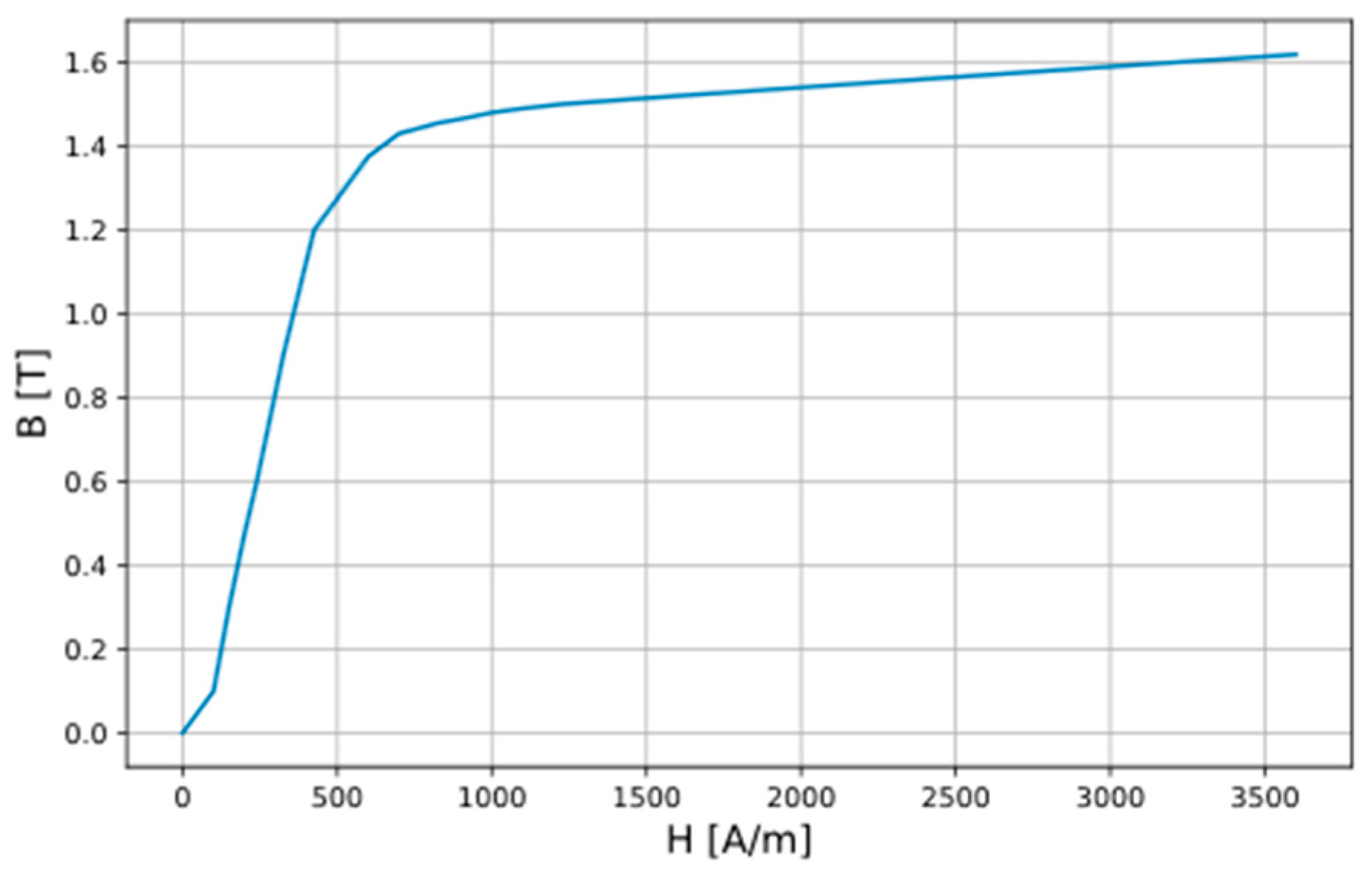
2.3. Partial Differential Equations of the Field and Its Integral Parameters

Performed magnetic field analysis assumed its quasi-stationarity, where time-varying phenomena and the eddy currents effects were omitted. This allows for the calculation time reduction, which is of great importance due to the multi-variant calculation’s nature, and simultaneously allows for compliance satisfactory for technical purposes. This limits the equations given in the second half of the 19th century by J.C. Maxwell and describes the electromagnetic field with Equations (5) and (6) given below [27].

$$\nabla \times \overrightarrow{\mathrm{H}}=\overrightarrow{\mathrm{j}}$$

(5)

$$\nabla \times \overrightarrow{\mathrm{E}}=0$$

(6)

The electromagnetic field equations can be solved using the $\overrightarrow{\mathrm{T}}-\mathsf{\Omega }$ potential method, where $\overrightarrow{\mathrm{T}}$ describes the electric potential vector and Ω the scalar magnetic potential. In the magnetostatic analysis, the potential $\overrightarrow{\mathrm{T}}$ is omitted, which simplifies the equation describing the intensity of the electromagnetic field to the form of Equation (7) [28].

$$\overrightarrow{\mathrm{H}}={\overrightarrow{\mathrm{H}}}_{\mathrm{S}}-\nabla \mathsf{\Omega }$$

(7)

$${\oint }_{\mathrm{l}}{\overrightarrow{\mathrm{H}}}_{\mathrm{S}}·\mathrm{d}\overrightarrow{\mathrm{l}}=\mathrm{ϴ}$$

(8)

The vector ${\overrightarrow{\mathrm{H}}}_{\mathrm{S}}$ (Equation (8)) describes the field intensity coming from the current density $\overrightarrow{\mathrm{J}}$ of the external source’s excitation and can be determined from the circuital law. The −∇Ω component is related to the ferromagnetic core material’s magnetization. Given the zero rotation value of this term, it can be expressed by the reduced scalar potential in the form −∇ϕ. Considering the above dependencies and substituting them to Equation (7), Expression (9) is obtained, which is solved in the sub-areas of air and the transformer windings [29,30].

$$-\nabla ·\left(\mathsf{\mu }\nabla \mathsf{\varphi }\right)+\nabla ·\left(\mathsf{\mu }{\overrightarrow{\mathrm{H}}}_{\mathrm{S}}\right)=0$$

(9)

In the transformer ferromagnetic area, due to the zero value of the current density external sources, Equation (10) is solved.

$$\nabla ·\left(\mathsf{\mu }\nabla \mathsf{\Omega }\right)=0$$

(10)

Knowledge of the distribution of magnetic potentials allows the calculation of their spatial derivatives in order to determine the components of the cartesian magnetic flux density vectors. However, the most relevant parameters are those calculated from the flux density vectors’ field integration. These are fluxes in the magnetic core and the leakage ones, stored energy, as well as windings inductances linked with the fluxes and magnetic forces. Assuming the flux density vector $\overrightarrow{\mathrm{B}}$ distribution in a surface $\mathrm{S}$, flux linkage with this surface can be determined via Equation (11).

$$\mathsf{\Psi }={\int }_{\mathrm{S}}\overrightarrow{\mathrm{B}}·\overrightarrow{\mathrm{d}\mathrm{S}}$$

(11)

Using the leakage energy stored in non-magnetic areas (Equation (12)), the transformer static leakage inductance can be determined from Expression (13). The dynamic leakage inductance in a linear environment can be determined using Equation (14) [31].

$$\mathrm{W}=\frac{1}{2\mathsf{\mu }}\left(\underset{\mathrm{V}}{\int }{\mathrm{B}}^2\mathrm{d}\mathrm{V}\right)$$

(12)

$${\mathrm{L}}_{\mathrm{r}\mathrm{s}}=\mathsf{\omega }\frac{2\mathrm{W}}{{\mathrm{I}}^2}$$

(13)

$${\mathrm{L}}_{\mathrm{r}\mathrm{d}}={\mathrm{L}}_{\mathrm{r}\mathrm{s}}+\mathrm{I}\frac{\partial {\mathrm{L}}_{\mathrm{r}\mathrm{s}}}{\partial \mathrm{I}}$$

(14)

The magnetic shunt inserted into the transformer window causes the division of the flux generated by the primary winding into two parts, in both the short-circuit and the no-load state. One of them closes through the magnetic shunt and is unrelated to the secondary winding, and the other part passes through this winding. Considering the above, the static (Equation (15)) and dynamic (Equation (16)) mutual inductance were calculated by forcing the current excitation only within the primary winding, simultaneously determining the value of the magnetic flux $\mathsf{\Psi }\left(\mathrm{I}\right)$ linked with the secondary winding.

$${\mathrm{L}}_{\mathsf{\mu }\mathrm{s}}=\frac{\mathsf{\Psi }\left(\mathrm{I}\right)}{\mathrm{I}}$$

(15)

$${\mathrm{L}}_{\mathsf{\mu }\mathrm{d}}=\frac{\partial \mathsf{\Psi }}{\partial \mathrm{i}}$$

(16)

3. Results of Field Analysis for Various Constructions and Partial Protrusion of the Magnetic Shunt

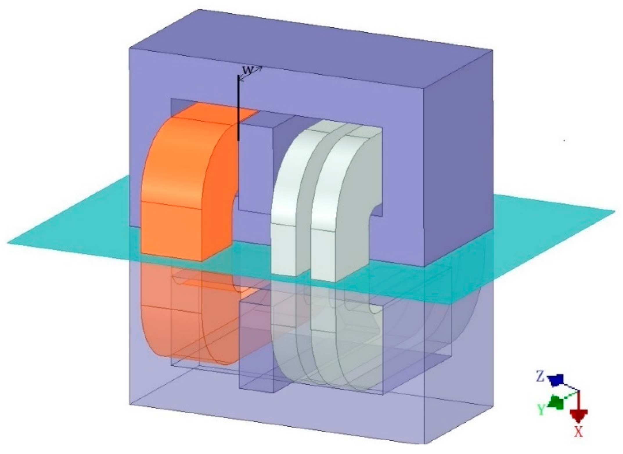
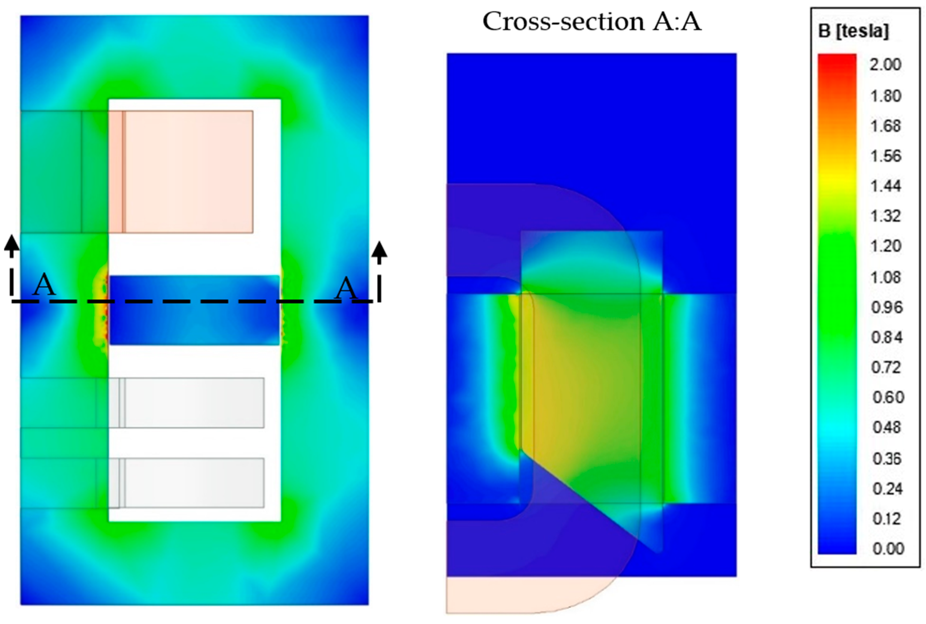
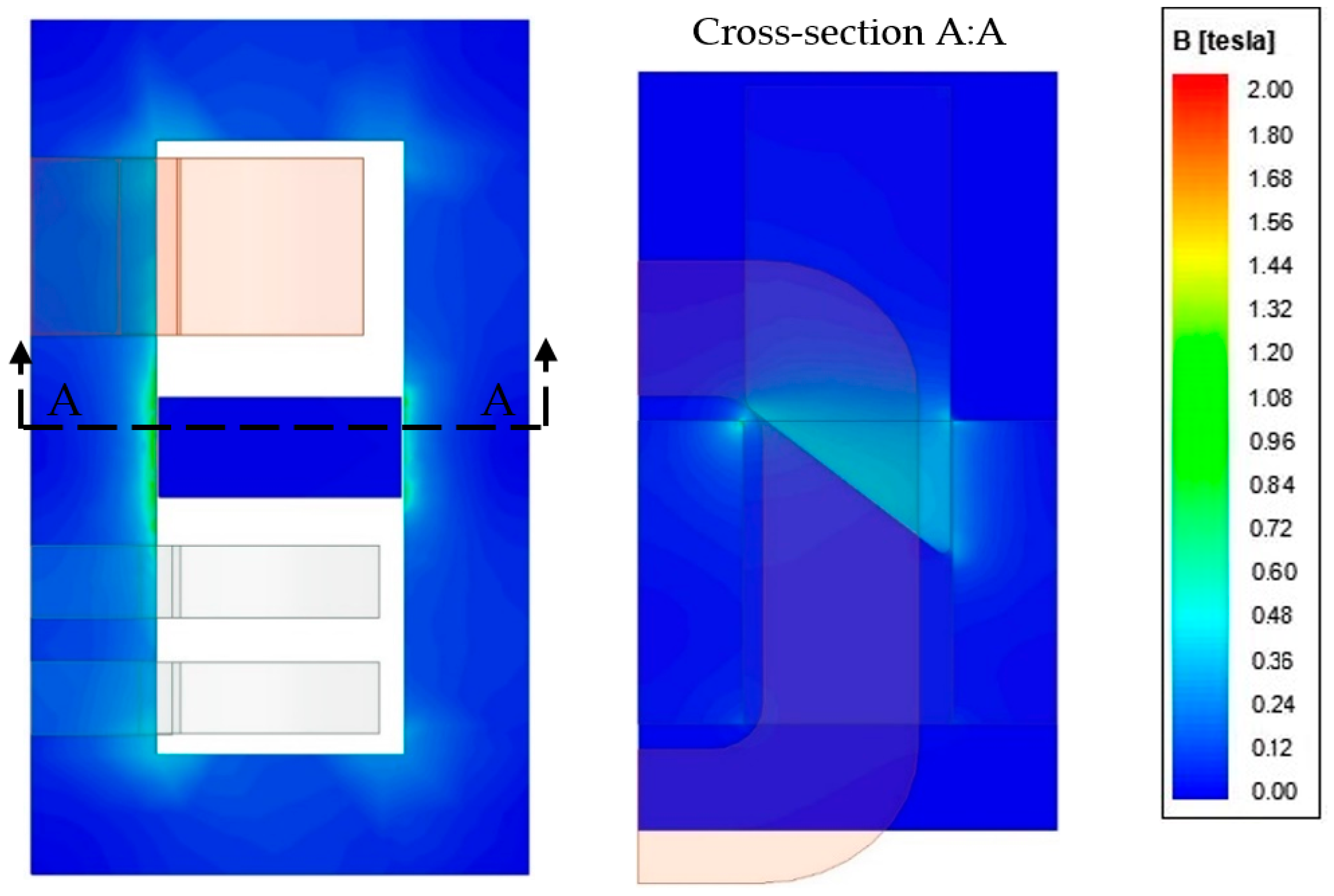
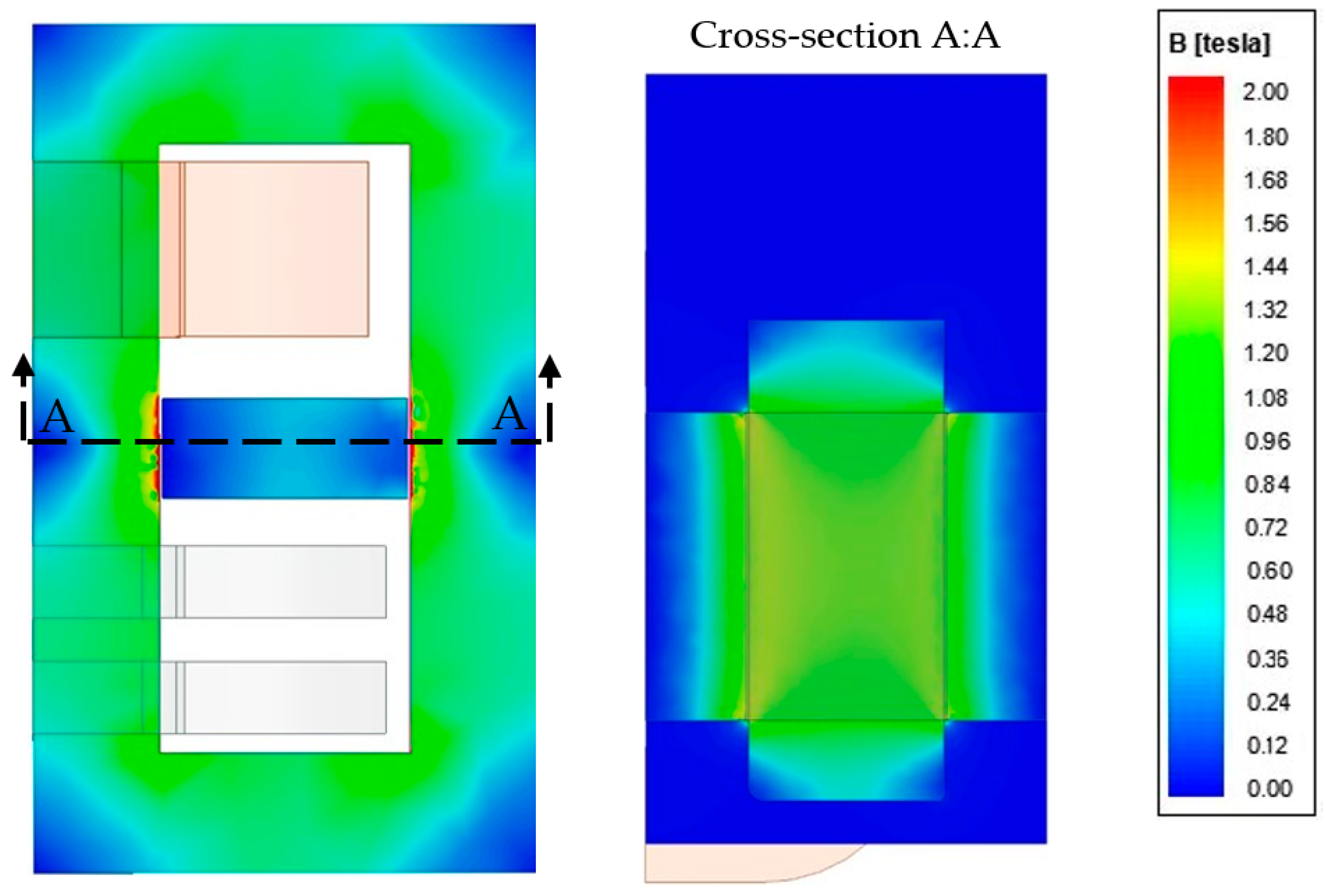
3.1. Magnetic Field in the Transformer with the Same Shunt Construction, but Its Different Protrusion from the Window

The performed magnetic field distribution analysis considered the primary winding current intensity in the range of 1–41 A and various positions of the beveled shunt fixes in the range of w = (20–180) mm. Figure 7 and Figure 8 show the magnetic flux density distribution for the two exemplary positions of the same shunt under the same ampere-turns for both the primary and secondary sides of the transformer windings. Due to the object symmetry, the distributions have been presented only for half of the transformer core, i.e., for one part of the shunt system. The current intensity value in the primary winding was equal to 9 A.

For the transformer short-circuit state, with no magnetic shunt presence or its complete pulling out, the flux generated by the primary winding is almost entirely compensated in the core by the secondary winding flux. Inserting the magnetic shunt into the transformer window allows some of the magnetic flux to flow through it. In Figure 7 and Figure 8, one can see the flux division into two parts: one closed by a magnetic shunt and the other one related to the secondary winding. The amount of flux flowing through the shunt depends on the ratio of the equivalent reluctance for the magnetic shunt with its two air gaps and the reluctance of the core part with the secondary winding. At a small shunt extraction, the flux divides into almost equal parts. With its pulling out the so-called hot spots, i.e., areas of shunt saturation, are visible. This is due to a relatively small cross-section of the shunt’s active parts.

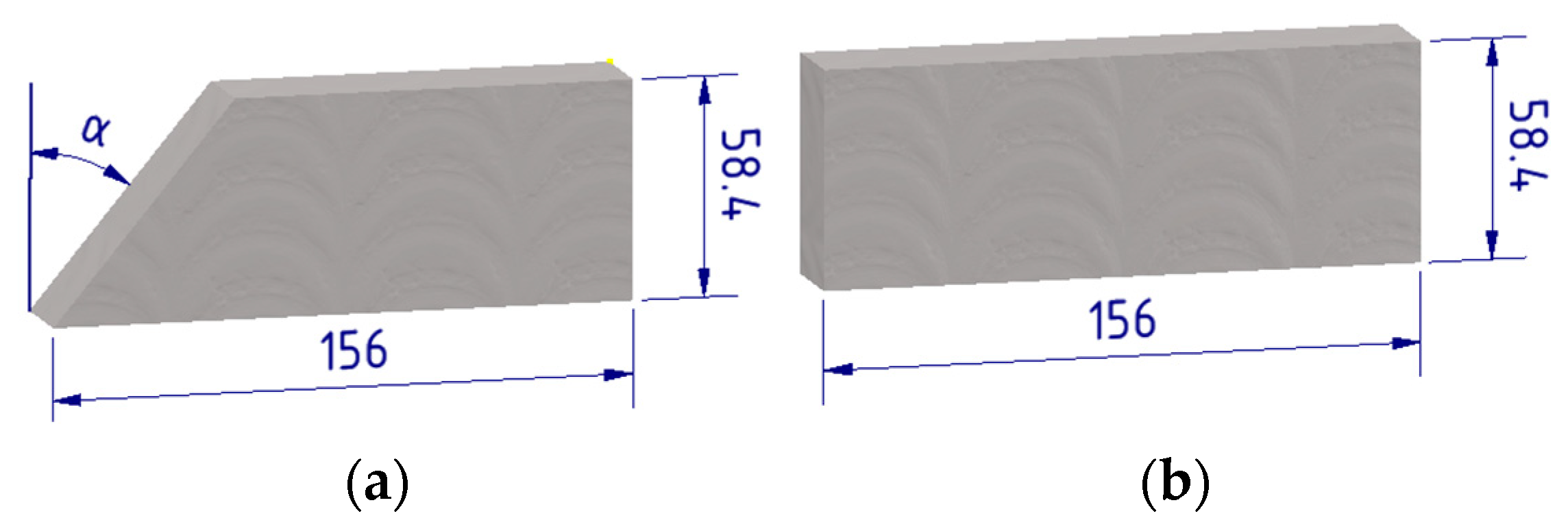
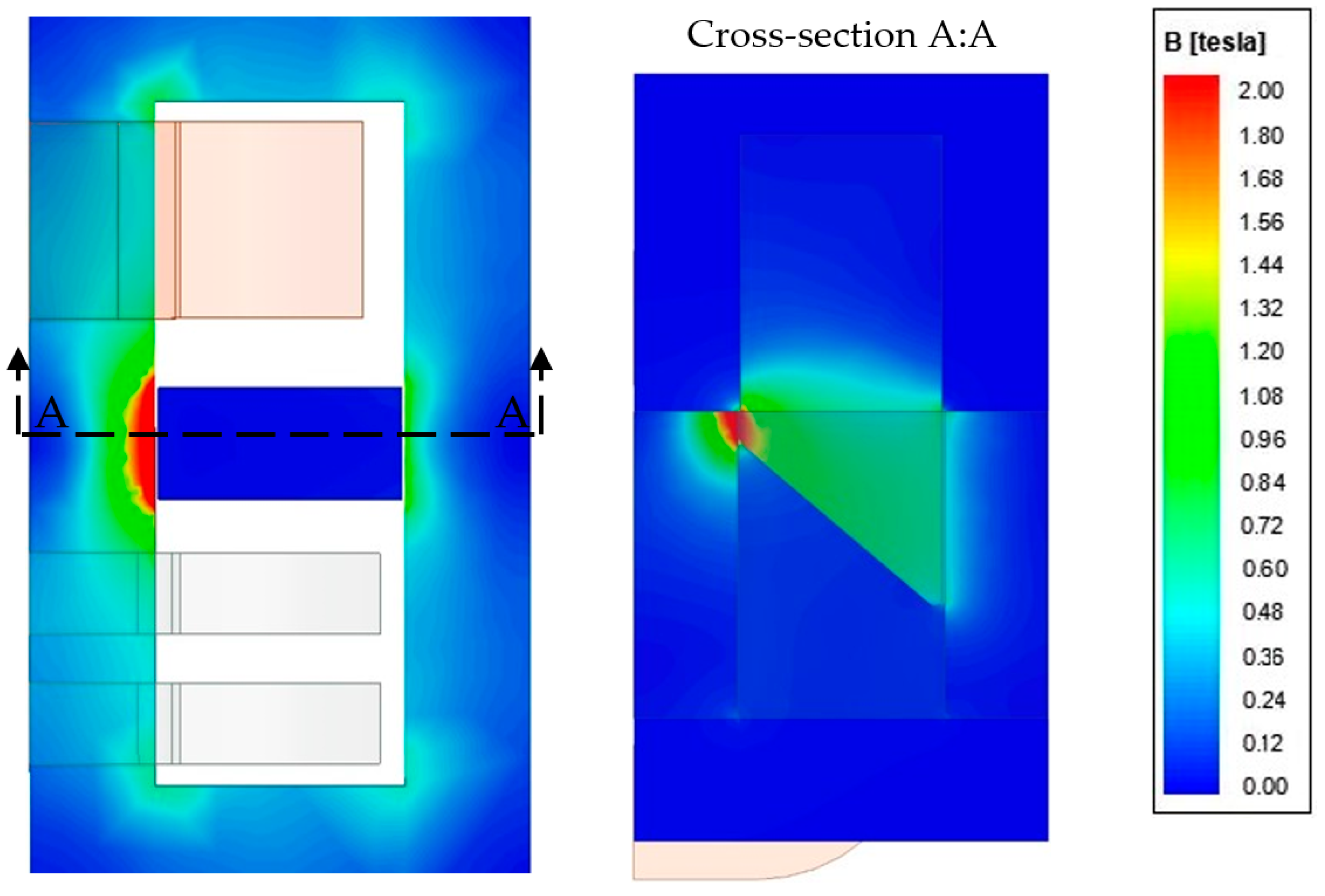
3.2. Field Simulation for Different Chamfering (Beveling) of the Magnetic Shunt

Figure 9, Figure 10, Figure 11 and Figure 12 show the magnetic flux density distribution in the half of the transformer core, magnetic shunt, and air gaps for beveled shunt exemplary positions. The first one presents the flux density histogram for the simple cuboidal shunt, which is the shunt geometry special case (α = 0°) mentioned above. The shunt extraction from the transformer window was equal to w = 30 mm. Figure 10 shows the flux density histogram for the same shunt extraction but beveled with the angle α = 45°.

Pulling the magnetic shunt out causes a part inside the transformer window and the core edges slightly saturation. For the cuboidal shunt (α = 0°) only, its slight saturation is visible on both sides; see Figure 11. For the beveled shunt, at this value of its protrusion, the magnetic “hot spot” (saturation) occurs only in the place of the shunt’s shorter surface inserted into the transformer window (Figure 12). This has a direct impact on the local construction overheating, so the temperature field analysis could be undertaken in further research.

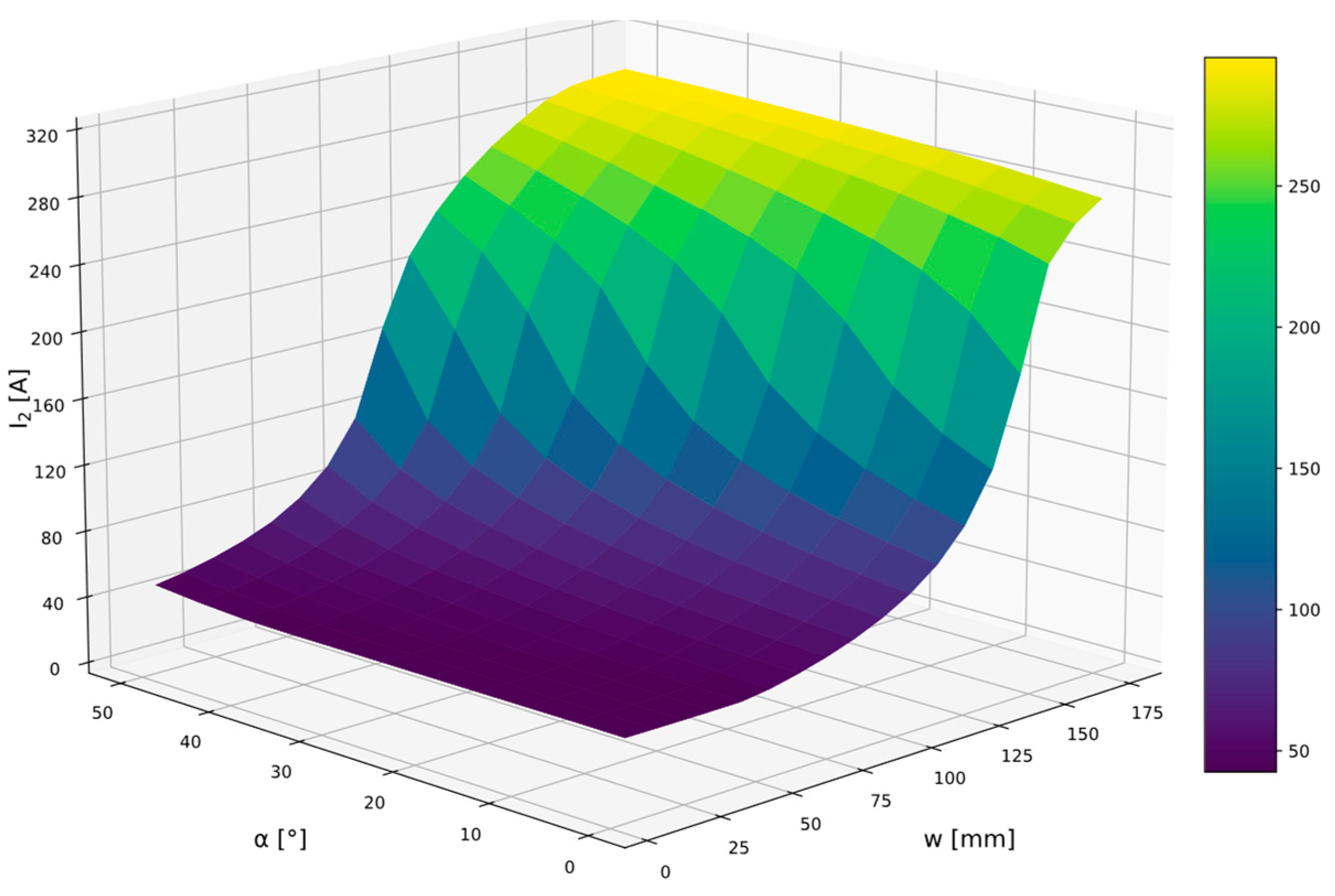
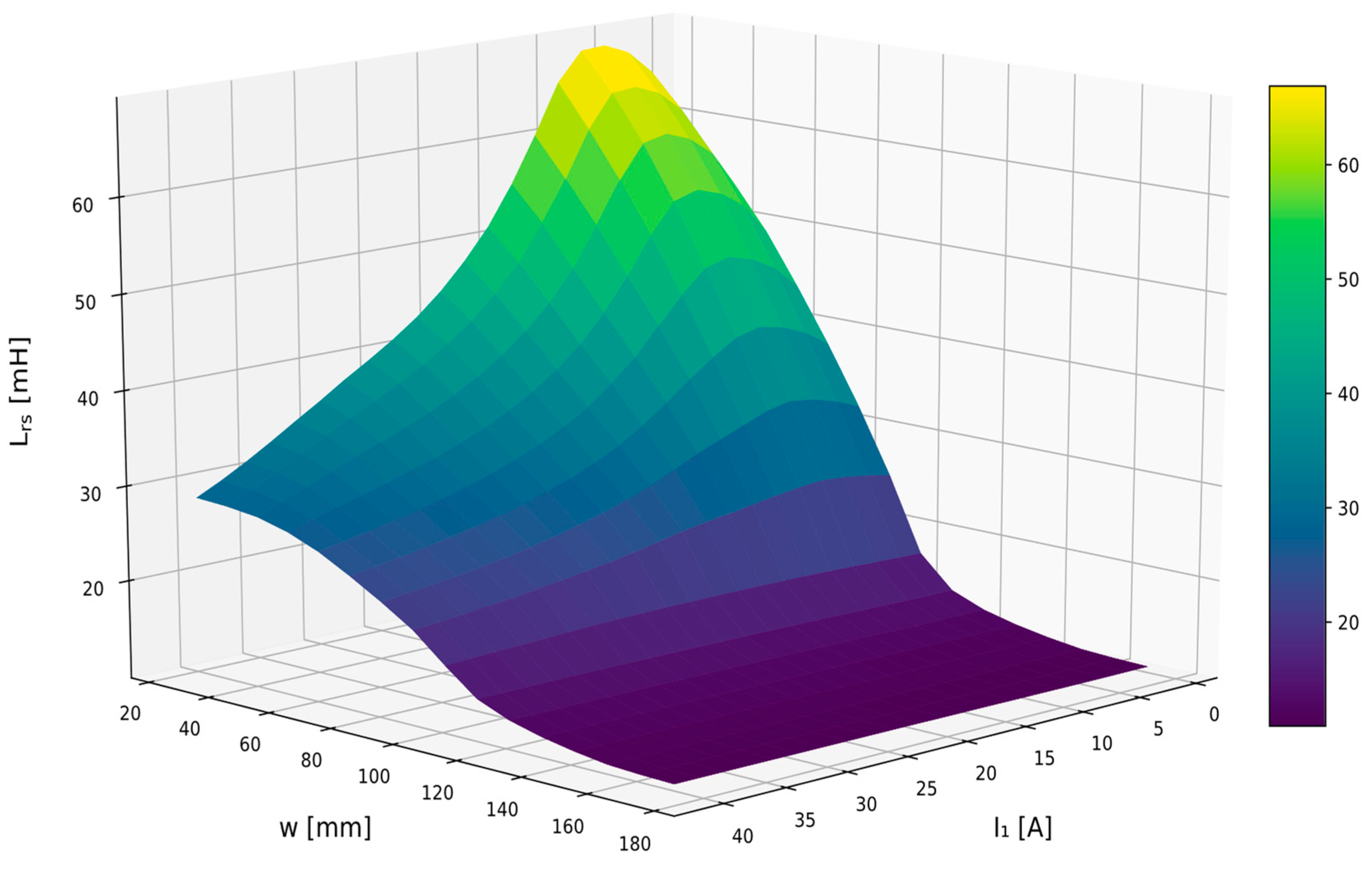
3.3. Short-Circuit Current and Leakage Reactance for Various Positions and Shunt Chamfering (Beveling)

Based on the magnetic field distribution, the transformer leakage reactance was determined for each beveling and shunt position. Based on this, the current I₂ related to the secondary winding was calculated, with the primary side powered with a voltage equal to 380 V. When the shunt is fully inserted into the transformer window, its beveling in the range of 0–20° does not affect transformer leakage reactance. Further angle α increasing shortens the active length of the shunt width located in the transformer window, which translates into a decrease in maximum leakage reactance value. This situation could be interpreted as an intermediate shunt position in the transformer window. On the opposite, for the extreme case when the magnetic shunt is fully extracted, the shunt beveling will have no significant effect on the leakage reactance, which is almost constant. Considering the above, at small bevel angles, the short-circuit reactance characteristic in the initial stage of shunt extraction is somewhat flattened. However, in the final phase of shunt extension, the reactance values change significantly. Beveling the shunt below 20 degrees does not affect the leakage reactance adjustment range. For bevel values above 20 degrees, the maximum leakage reactance value decreases, reducing the adjustment range while increasing the smoothness of the secondary winding short-circuit current regulation. The reactance changes impact strongly the short-circuit current intensity I₂, which is visible in Figure 13.

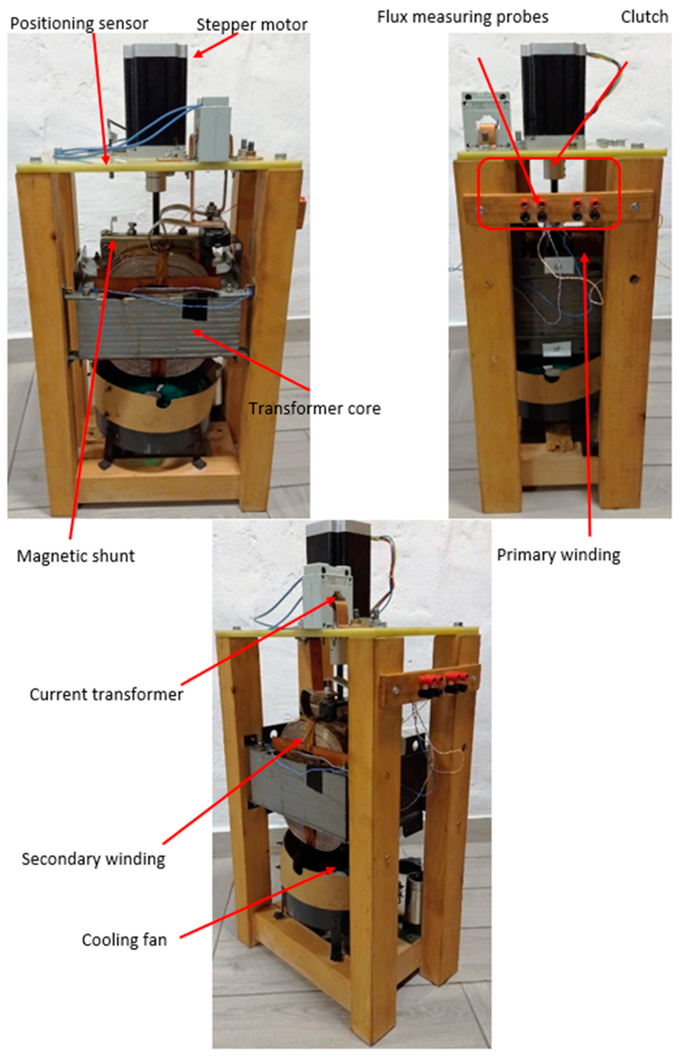
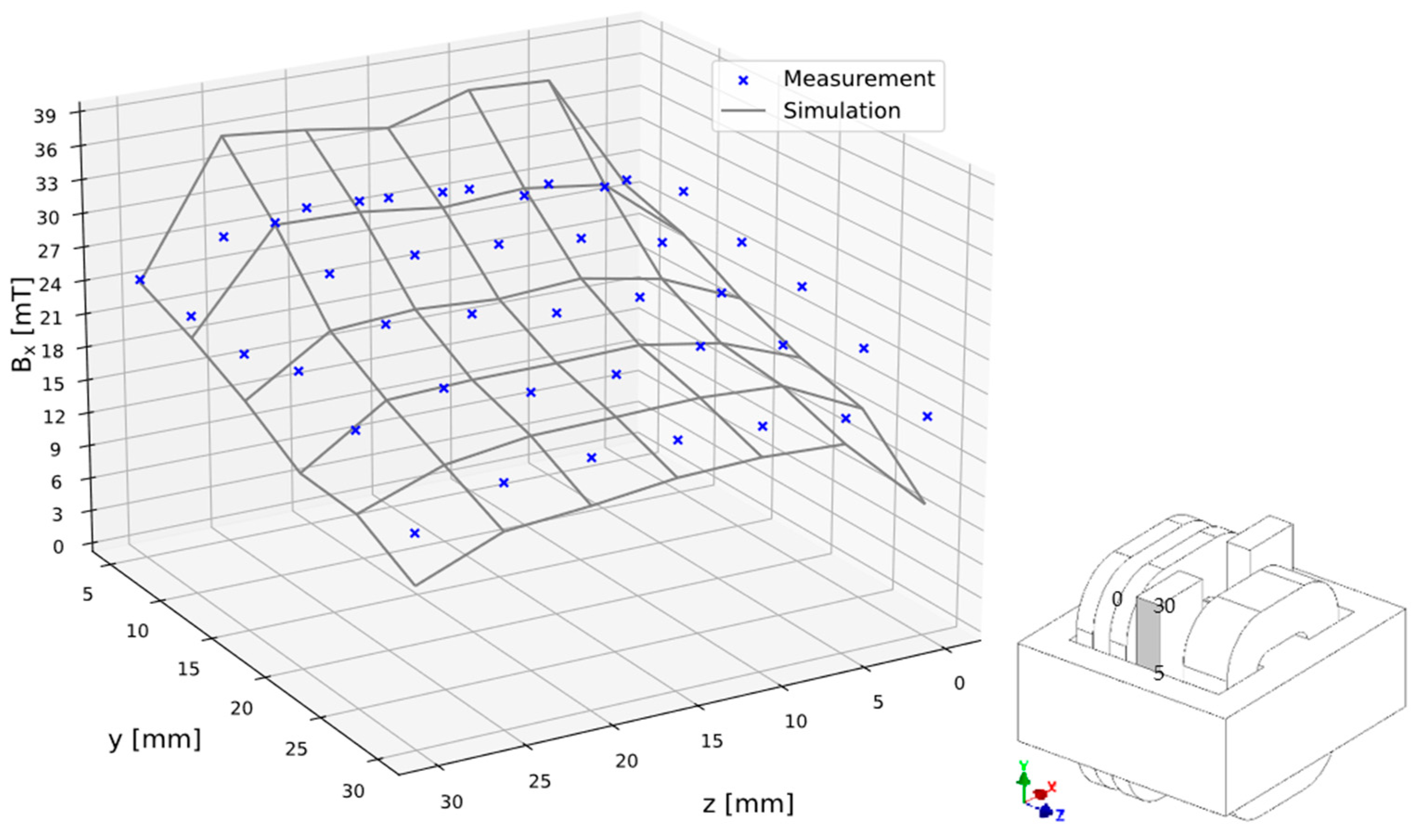
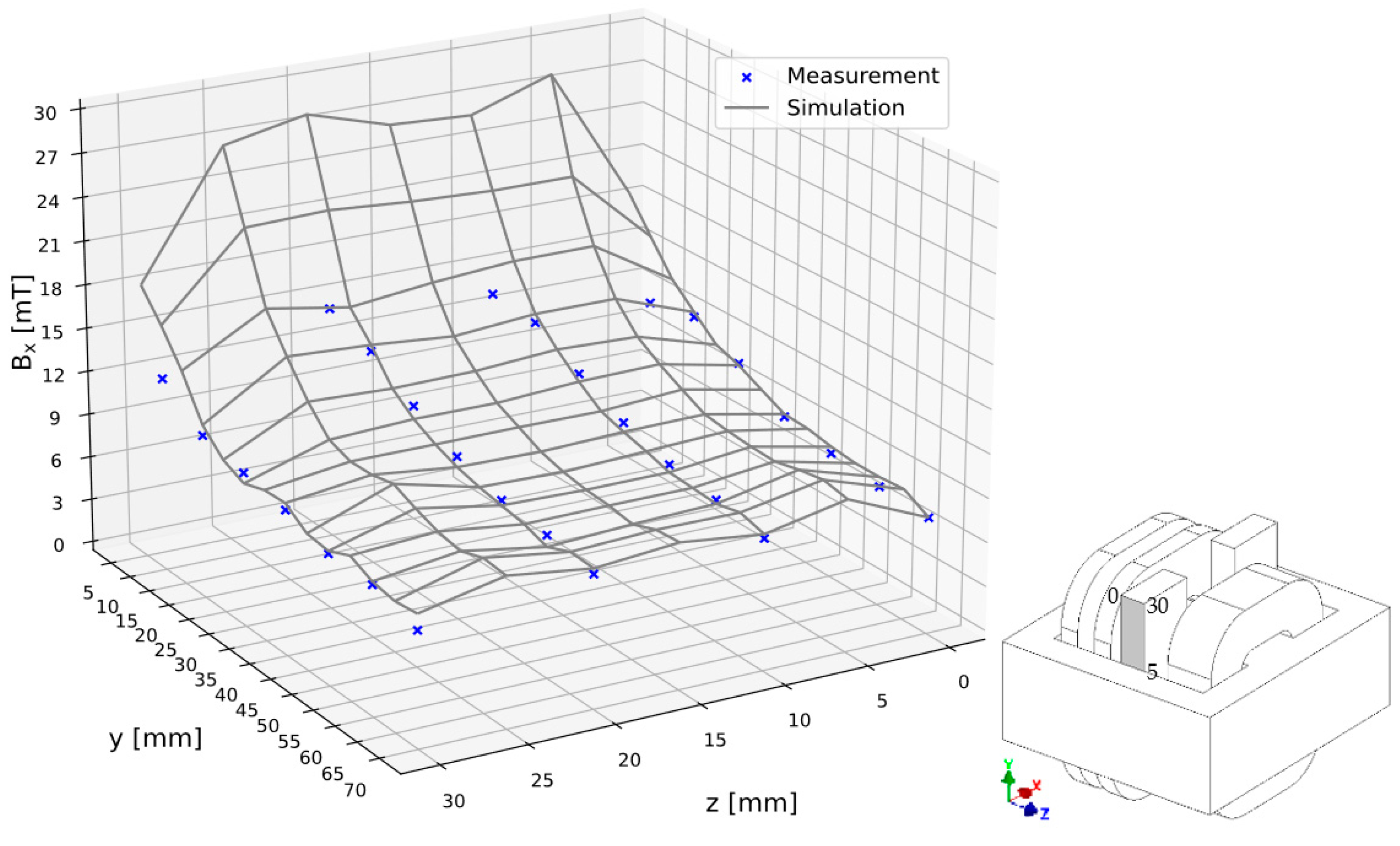
4. Measurement Verification of the Simulations

The proposed simulation model of the described transformer was verified by comparing the flux density distributions at the chosen leakage zone points and by comparing the most important integral parameter of the electromagnetic field—transformer leakage reactance. The first verification allows for a detailed assessment of the quality of the mathematical model and works very well in finding the so-called magnetic hot spots. However, a comprehensive local errors assessment would require measurements of all magnetic flux density vector components for the entire transformer leakage zone. Therefore, due to the multitude of variants of shunt positions, and current excitation, the comparison of the calculated and measured leakage reactance values was chosen as the main criteria for evaluating the model quality. Figure 14 shows the tested object with instruments that enable performing precise tests related to the magnetic shunt positioning in the transformer window.

4.1. Comparison of Three-Dimensional Magnetic Flux Density Distribution

The magnetic flux density vector components distribution comparison was limited to the magnetic shunt outer plane; see Figure 15 and Figure 16. Their values in this area reflect the field’s asymmetric nature concerning the XZ plane. The flux density values comparison was made in the short-circuit state at 4.5 mm from the shunt ferromagnetic surface, under the constant ampere-turns of the windings current flow equal ϴ = 1020 A. The current value was selected considering the possibility of forcing the same flux density for a transformer with a fully inserted shunt, as well as for a transformer without a magnetic shunt. The comparison was limited to the normal component since it has a major impact on the field’s nature. The principal differences between the measured values and those obtained during simulation were at the outer edges of the magnetic shunt and close to the transformer core edges. These differences are due to the higher contribution of the remaining components of the magnetic flux density vector due to the inaccuracy of the probe mounting. This problem is highlighted at a small magnetic shunt extraction, where there is a large variability in the direction of the magnetic field force lines and the flux density values on a small core segment area.

Figure 15 and Figure 16 show the distribution of the normal to the magnetic shunt, Bx components on the outer shunt surface, obtained on the simulation basis along with the marked values at the measure points, with the pulling shunt out from the transformer window equal to 30 mm and 70 mm, respectively.

4.2. Comparison of the Leakage Reactances

One of the transformer’s magnetic field integral parameters is its leakage inductance associated with each winding. By calculating the leakage energy stored in nonmagnetic objects, it is impossible to directly determine the part of the energy associated with a specific winding. So, these inductances could be calculated by assuming that the leakage reactance of the primary and secondary transformer windings are equal. Based on the magnetic field distribution, the static leakage inductance related to the primary winding was determined from the Expression (13), Figure 17. The static inductance associated with the secondary winding was calculated with the square of the turn’s ratio ${{(N}_2/N_1)}^2$ and is considerably smaller, see Figure 18.

The leakage reactance values comparison allows for a comprehensive evaluation of the field model. Figure 19a,b show the calculated and measured values of the windings’ leakage reactance transferred to the primary side.

Table 2 shows the relative error calculated from Expression (17), depending on magnetic shunt extraction w in relation to the transformer window and the primary winding current I₁.

$${\mathsf{\delta }}_{{\mathrm{X}}_{\mathrm{r}}}=\left|\frac{{{\mathrm{X}}_{\mathrm{r}}}_{\mathrm{s}\mathrm{y}\mathrm{m}}-{{\mathrm{X}}_{\mathrm{r}}}_{\mathrm{m}\mathrm{e}\mathrm{s}}}{{{\mathrm{X}}_{\mathrm{r}}}_{\mathrm{m}\mathrm{e}\mathrm{s}}}\right|·100\mathrm{\%}$$

(17)

where:

• ${{\mathrm{X}}_{\mathrm{r}}}_{\mathrm{s}\mathrm{y}\mathrm{m}}$—calculated leakage reactance;
• ${{\mathrm{X}}_{\mathrm{r}}}_{\mathrm{m}\mathrm{e}\mathrm{s}}$—measured leakage reactance.

Table 2. Percentage relative error value δ_Xr calculated at each measurement point.

Extraction w [mm]	Primary Winding Current Intensity in Amps
	1	3	5	7	9	11	13	15	17	19
25	7.4%	2.2%	1.3%	5.7%	11.1%	-	-	-	-	-
35	8.6%	3.5%	0.5%	4.9%	9.7%	-	-	-	-	-
45	5.6%	2.9%	0.7%	4.7%	9.1%	10.6%	-	-	-	-
55	5.6%	3.1%	0.7%	4.5%	8.3%	9.5%	-	-	-	-
65	3.5%	3.7%	0.2%	3.3%	6.7%	8.5%	9%	8.7%	-	-
75	4.3%	3.5%	0.8%	2.2%	5.3%	7.1%	8.4%	8.6%	8.5%	8.4%
85	5.1%	4.5%	2%	0%	2.8%	4.7%	6.6%	7.8%	8.1%	8.4%

Table 2. Percentage relative error value δ_Xr calculated at each measurement point.

Extraction w [mm]	Primary Winding Current Intensity in Amps
	1	3	5	7	9	11	13	15	17	19
25	7.4%	2.2%	1.3%	5.7%	11.1%	-	-	-	-	-
35	8.6%	3.5%	0.5%	4.9%	9.7%	-	-	-	-	-
45	5.6%	2.9%	0.7%	4.7%	9.1%	10.6%	-	-	-	-
55	5.6%	3.1%	0.7%	4.5%	8.3%	9.5%	-	-	-	-
65	3.5%	3.7%	0.2%	3.3%	6.7%	8.5%	9%	8.7%	-	-
75	4.3%	3.5%	0.8%	2.2%	5.3%	7.1%	8.4%	8.6%	8.5%	8.4%
85	5.1%	4.5%	2%	0%	2.8%	4.7%	6.6%	7.8%	8.1%	8.4%

5. Discussion

The field distribution analysis was started by determining (based on the simulations) the smallest size of three-dimensional computational space that one should consider during transformer field distribution calculation, as in Figure 3. Then, to increase the field analysis accuracy and reduce the computational costs, the symmetry plane was applied, which reduced the field analysis to half the area of the leakage region.

A comparison of the magnetic flux density components distribution confirmed the asymmetric nature of the magnetic field for intermediate magnetic shunt positions. Pulling the shunt out of the transformer window pulls the magnetic field behind it, causing its asymmetric distribution, which makes it impossible to use the symmetry with respect to the XZ plane; see Figure 15 and Figure 16. The above is confirmed by both the simulation and measurement results.

In the leakage field sub-areas characterized by relatively lower magnetic flux density values, good agreement between simulation and performed measurements was obtained, mainly due to smaller measurement errors related to the influence of other magnetic flux density vector components, which are presented in Figure 15 and Figure 16. Magnetic flux density components values comparison allows for assessing the object’s mathematical model quality. However, a comprehensive assessment would require measurements of all magnetic flux density vector components for the entire transformer leakage area. Therefore, due to variants multitude, shunt positions, and current excitation, the determined and measured leakage reactance value comparison was chosen as the principal criterion for evaluating field model quality, performed as part of measurement verification.

The average percentage relative error between calculated and measured transformer leakage reactance values equals 5.4%. Considering performed simplifications, which included physical model dimensions averaging, assumption of air gap equality in the entire magnetic shunt positions range, as well as computational area limitation, a good agreement with the measured values was obtained, which confirms the correctness of the used method and the assumed symmetry conditions for the leakage zone.

In the HLR transformers with increased leakage reactance and the movable magnetic shunt, the main factor limiting the short-circuit current is its leakage reactance, which mainly depends on the magnetic shunt position in the transformer window, Figure 19. It reaches a maximum value for a fully inserted into the transformer window magnetic shunt and the minimum value when the transformer is without the shunt. The maximum value of the leakage reactance for the considered transformer equals 43.3 Ω and the minimal value 6.8 Ω, which gives a six-fold change in the short-circuit current in the entire adjustment range.

Increasing the shunt bevel angle α improves secondary winding current regulation linearity. Changes in this angle from 0° to 20° have almost no effect on the maximum leakage reactance value, but at the same time, they only slightly improve the above-mentioned regulation linearity. Due to the constant magnetic shunt length, further angle α increases, causing the maximum reactance value to decrease, while transformer short-circuits current control linearity is improved, Figure 13.

6. Conclusions

Three-dimensional field analysis enables the magnetic field distribution simulation of an HLR transformer with a movable magnetic shunt. This makes it possible to determine its static and dynamic characteristics over the entire range of magnetic shunt positions. The numerical calculations results give good (for technical purposes) compliance with the measurements, which confirms the developed model’s correctness. This allows for determining the mentioned key parameters without the need to build expensive prototypes or perform time-consuming analytical calculations. Although the magnetic flux flowing through the magnetic shunt, inserted in the transformer window, forces the non-linear characteristic of the leakage inductance, the short circuit current control is effective. The magnetic shunt enables smooth regulation of the secondary winding current in a wide range.

Analysis of the magnetic field distribution showed that pulling the magnetic shunt out from the transformer window results in saturation of its core and shunt corner. This leads to the appearance of so-called “hot spots”. A thermal analysis covering the above phenomenon will allow the design of an appropriate cooling system and maybe a conducted research continuation.

References

1. Alves, B.S.; Kuo-Peng, P.; Dular, P. Contribution to power transformers leakage reactance calculation using analytical approach. Int. J. Electr. Power Energy Syst. 2019, 105, 470–477. [Google Scholar] [CrossRef]
2. Dawood, K.; Cinar, M.A.; Alboyaci, B.; Sonmez, O. A new method for the calculation of leakage reactance in power transformers. J. Electr. Eng. Technol. 2017, 12, 1883–1890. [Google Scholar] [CrossRef]
3. Jamali, S.; Nasir, K.; Abbaszadeh, K.; Arand, S.J. The Study of Magnetic Flux Shunts Effects on the Leakage Reactance of Transformers via FEM. Majlesi J. Electr. Eng. 2010, 4, 47–52. [Google Scholar] [CrossRef]
4. Hayes, J.G.; O’Donovan, N.; Egan, M.G.; O’Donnell, T. Inductance characterization of high-leakage transformers. In Proceedings of the Conference Proceedings—IEEE Applied Power Electronics Conference and Exposition—APEC, Miami Beach, FL, USA, 9–13 February 2003; Volume 2, pp. 1150–1156. [Google Scholar]
5. Grossner, N.R. The Geometry of Regulating Transformers. IEEE Trans. Magn. 1978, 14, 87–94. [Google Scholar] [CrossRef]
6. Koteras, D.; Tomczuk, B.; Waindok, A. Implicit iteration calculations using 3D field analyses, to predict the power loss in powder ferromagnets, with their measurement tests. Measurements 2023, 207, 112311. [Google Scholar] [CrossRef]
7. Tomczuk, B.; Koteras, D. Magnetic flux distribution in the amorphous modular transformers. J. Magn. Magn. Mater. 2011, 323, 1611–1615. [Google Scholar] [CrossRef]
8. O’Connor, P. Test Engineering: A Concise Guide to Cost-Effective Design, Development and Manufacture; John Wiley & Sons: Hoboken, NJ, USA, 2001. [Google Scholar]
9. Güemes-Alonso, J.A. A new method for calculating of leakage reactances and iron losses in transformers. In Proceedings of the ICEMS’2001, Fifth International Conference on Electrical Machines and Systems, Shenyang, China, 18–20 August 2001; Volume 1, pp. 178–181. [Google Scholar]
10. Kashtiban, A.M.; Hagh, M.T.; Milani, A.R.; Haque, M.T. Finite Element Calculation of Winding Type Effect on Leakage Flux in SinglePhase Shell Type Transformers. In Proceedings of the 5th WSEAS International Conference on Applications of Electrical Engineering, Prague, Czech Republic, 12–14 March 2006; pp. 39–43. [Google Scholar]
11. Jahromi, A.N.; Faiz, J.; Mohseni, H. A fast method for calculation of transformers leakage reactance using energy technique. IJE Trans. B Appl. 2003, 16, 41–48. [Google Scholar]
12. Mechkov, E.; Tzeneva, R.; Mateev, V.; Yatchev, I. Thermal analysis using 3D FEM model of oil-immersed distribution transformer. In Proceedings of the 19th International Symposium on Electrical Apparatus and Technologies (SIELA), Bourgas, Bulgaria, 29 May–1 June 2016. [Google Scholar]
13. Ahmad, A.; Javed, I.; Nazar, W.; Mukhtar, M.A. Short Circuit Stress Analysis Using FEM in Power Transformer on H-V Winding Displaced Vertically & Horizontally. Alex. Eng. J. 2018, 57, 147–157. [Google Scholar]
14. Naranpanawe, L.; Saha, T.; Ekanayake, C. Finite element analysis to understand the mechanical defects in power transformer winding clamping structure. In Proceedings of the IEEE Power & Energy Society General Meeting, Chicago, IL, USA, 16–20 July 2017; pp. 1–5. [Google Scholar]
15. Gowri, N.V.; Akthar, Z. Finite Element Analysis of Power Transformer. Int. J. Mech. Eng. Technol. (IJMET) 2019, 10, 1384–1391. [Google Scholar]
16. Sieradzki, S.; Rygal, R.; Soiński, M. Apparent Core Losses and Core Losses in Five-Limb Amorphous Transformer of 160 kVA. IEEE Trans. Magn. 1998, 3, 1189–1191. [Google Scholar] [CrossRef]
17. Mousavi, S.; Shamei, M.; Siadatan, A.; Nabizadeh, F.; Mirimani, S.H. Calculation of Power Transformer Losses by Finite Element Method. In Proceedings of the IEEE Electrical Power and Energy Conference (EPEC), Toronto, ON, Canada, 10–11 October 2018; pp. 1–5. [Google Scholar] [CrossRef]
18. Zaitsev, I.; Bereznychenko, V.; Bajaj, M.; Taha, I.B.M.; Belkhier, Y.; Titko, V.; Kamel, S. Calculation of Capacitive-Based Sensors of Rotating Shaft Vibration for Fault Diagnostic Systems of Powerful Generators. Sensors 2022, 22, 1634. [Google Scholar] [CrossRef] [PubMed]
19. Tomczuk, B. Calculation of the Magnetic Field and Short-Circuit Reactance of Dissipation Transformers. Ph.D. Thesis, Lodz University of Technology, Lodz, Poland, 1985. [Google Scholar]
20. Zakrzewski, K.; Tomczuk, B. Application of the finite difference method for the windings reactance calculations of the stray transformers. Arch. Elektrotechniki PWN 1990, 37, 43–50. (In Polish) [Google Scholar]
21. Tomczuk, B. Three-Dimensional Leakage Reactance Calculation and Magnetic Field Analysis for Unbounded Problems. IEEE Trans. Magn. 1992, 28, 1935–1940. [Google Scholar] [CrossRef]
22. Tomczuk, B. Analysis of 3-D Magnetic Fields in High Leakage Reactance Transformers. IEEE Trans. Magn. 1994, 30, 2734–2738. [Google Scholar] [CrossRef]
23. Kulkarni, S.V.; Khaparde, S.A. Transformer Engineering: Design, Technology, and Diagnostics, 2nd ed.; CRC Press: Boca Raton, FL, USA, 2012. [Google Scholar]
24. Ansys Maxwell 3D User’s Guide. Available online: https.www.ansys.com/ (accessed on 13 June 2023).
25. Binns, K.J.; Lawrenson, P.J.; Trowbridge, C.W. The Analytical and Numerical Solution of Electric and Magnetic Fields; John Wiley and Sons: New York, NY, USA, 1993. [Google Scholar]
26. Sykulski, J.K. Computational Magnetics; Chapman & Hall: London, UK, 1995. [Google Scholar]
27. Bandelier, B.; Rioux-Damidau, F. Mixed finite element method for magnetostatics in ℝ3. IEEE Trans. Magn. 1998, 34, 2473–2476. [Google Scholar] [CrossRef]
28. Li, Y.; Berthiau, G.; Feliachi, M.; Cheriet, A. 3D finite volume modeling of ENDE using electromagnetic T-formulation. J. Sens. 2012, 2012, 785271. [Google Scholar] [CrossRef]
29. Specogna, R.; Suuriniemi, S.; Trevisan, F. Geometric T-Ω approach to solve eddy currents coupled to electric circuits. Int. J. Numer. Methods Eng. 2008, 74, 101–115. [Google Scholar] [CrossRef]
30. Codecasa, L.; Dular, P.; Specogna, R.; Trevisan, F. A perturbation method for the T- ω geometric eddy-current formulation. IEEE Trans. Magn. 2010, 46, 3045–3048. [Google Scholar] [CrossRef]
31. Farahani, H.F.; Zare, M.; Mohammad, S.; Razi, P.; Khodakarami, A. Finite Element Analysis of Leakage Inductance of 3-Phase Shell-Type and Core Type Transformers. Res. J. Appl. Sci. Eng. Technol. 2012, 4, 1721–1728. [Google Scholar]
Figure 1. The HLR transformer with radial magnetic leakage.
Energies 16 06814 g001
Figure 2. Transformer in the computing area.
Energies 16 06814 g002
Figure 3. Dependence of the calculated energy stored in the outer leakage field area on the calculation cube edge length “k”, for the extracted shunt (a), and the fully inserted shunt (b).
Energies 16 06814 g003
Figure 4. The HLR transformer with symmetry boundary.
Energies 16 06814 g004
Figure 5. B-H Curve of the M530—50A steel.
Energies 16 06814 g005
Figure 6. Magnetic shunt with chamfering angle (a), and without chamfering angle (b).
Energies 16 06814 g006
Figure 7. Magnetic flux density distribution in the transformer core and the leakage zone, for the beveled edges of magnetic shunt, pulled out by w = 20 mm and the current intensity in the primary winding of 9 A.
Energies 16 06814 g007
Figure 8. Flux density for pulled the beveled shunt out of the transformer window by 110 mm, and the current intensity in the primary winding of 9 A.
Energies 16 06814 g008
Figure 9. Flux density in the transformer and leakage zone for 30 mm extraction of the cuboidal magnetic shunt ( α = 0°).
Energies 16 06814 g009
Figure 10. Flux density in the transformer core and leakage zone for 30 mm magnetic shunt extraction and α = 45°.
Energies 16 06814 g010
Figure 11. Flux density in transformer and leakage zone for w = 90 mm magnetic shunt extraction without beveling ( α = 0°).
Energies 16 06814 g011
Figure 12. Leakage flux density for w = 90 mm magnetic shunt extraction and the shunt ( α = 45°).
Energies 16 06814 g012
Figure 13. Short second current intensity in function of beveling and shunt extraction.
Energies 16 06814 g013
Figure 14. Object test setup with measurement instruments.
Energies 16 06814 g014
Figure 15. Comparison of the simulated and measured Bx values, of the flux density vector at the points for 4.5 mm from the shunt surface for w = 30 mm of the magnetic shunt extraction.
Energies 16 06814 g015
Figure 16. Comparison of the simulated and measured Bx values, of the flux density vector at the points for 4.5 mm from the shunt surface for w = 70 mm of the magnetic shunt extraction.
Energies 16 06814 g016
Figure 17. Calculated transformer primary winding static leakage inductance.
Energies 16 06814 g017
Figure 18. Calculated transformer secondary winding static leakage inductance.
Energies 16 06814 g018
Figure 19. Leakage reactance transferred to the transformer primary winding, calculated values (a), measured ones (b).
Energies 16 06814 g019