
Gust Modeling with State-of-the-Art Computational Fluid Dynamics (CFD) Software and Its Influence on the Aerodynamic Characteristics of an Unmanned Aerial Vehicle


Abstract
:1. Introduction
- First, the steady-state aerodynamic characteristics were determined experimentally using a wind tunnel and numerically using ANSYS Fluent Release 16.2 software. The experimental results allowed the numerical model to be validated;
- After obtaining a satisfactory convergence in the results, numerical calculations analyzing the impact of gusts on the aerodynamic characteristics of a UAV were performed. Time-dependent boundary conditions determined with the so-called user-defined functions (UDFs) were proposed to simulate the gust.
2. Materials and Methods
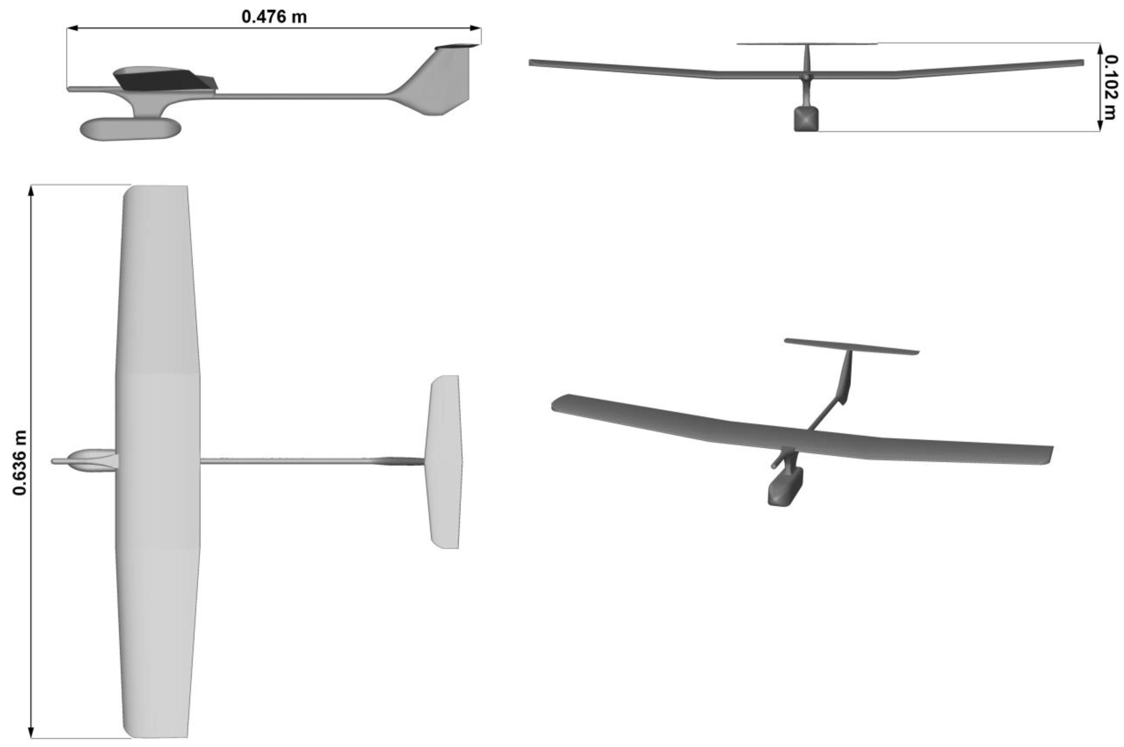
2.1. Model under Examination
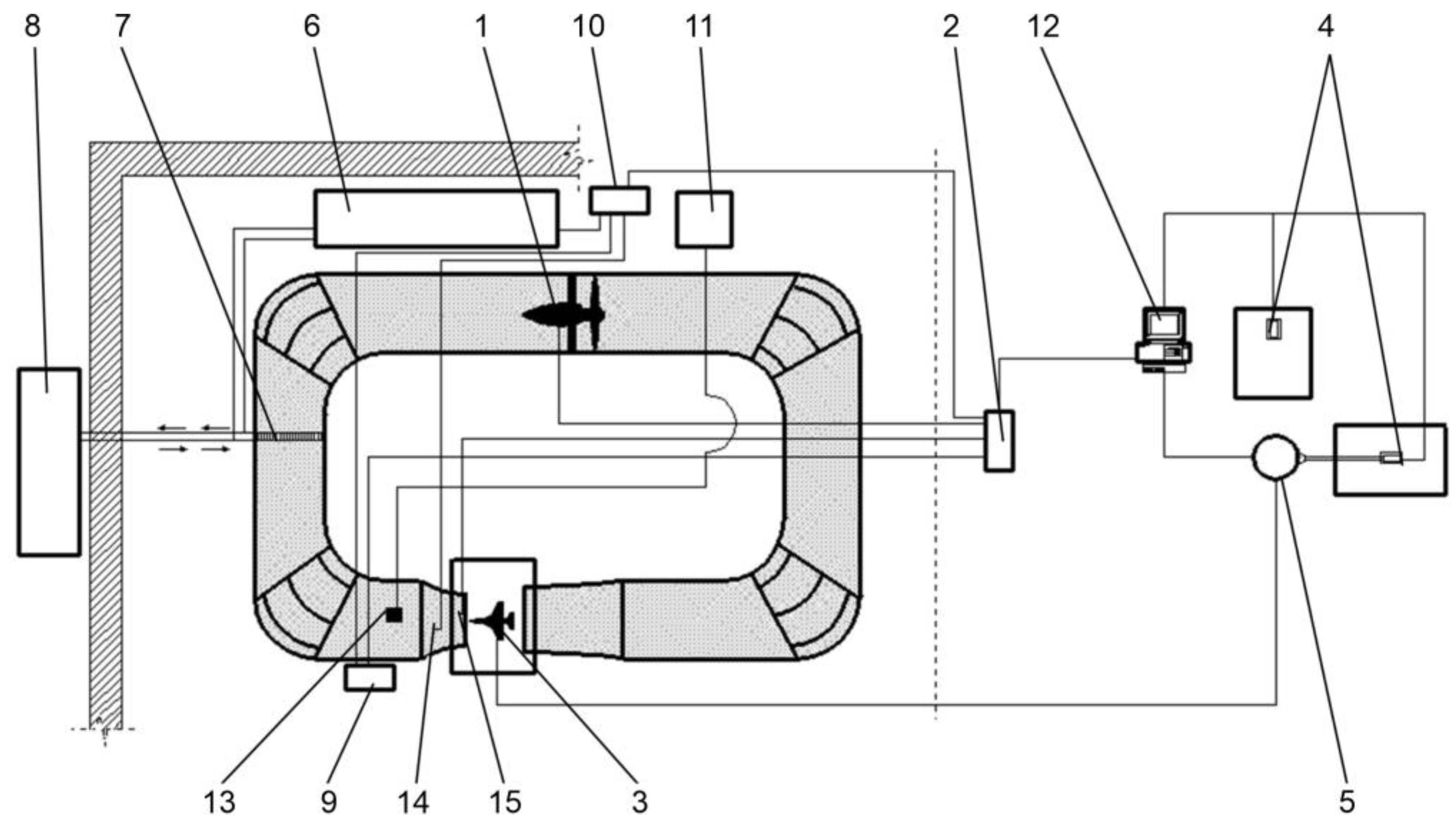
2.2. Measurement System for Experimental Investigation
2.3. CFD Calculations
2.3.1. Governing Equations
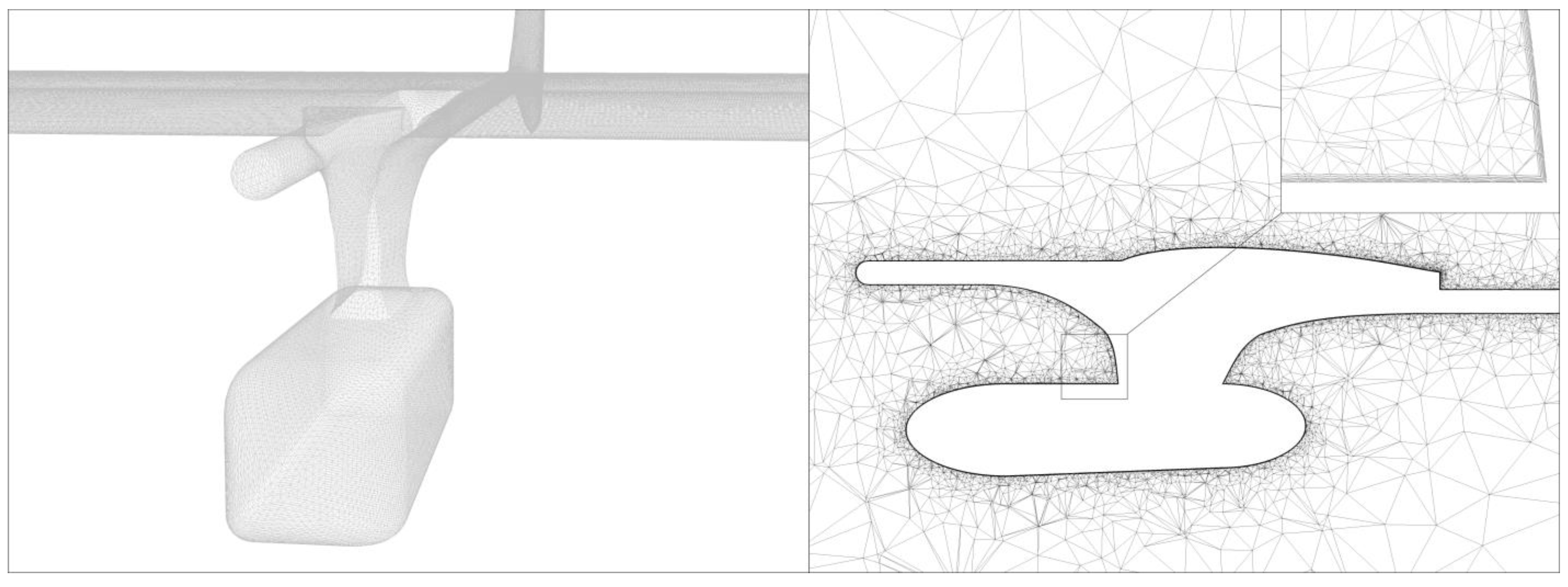
2.3.2. Numerical Model
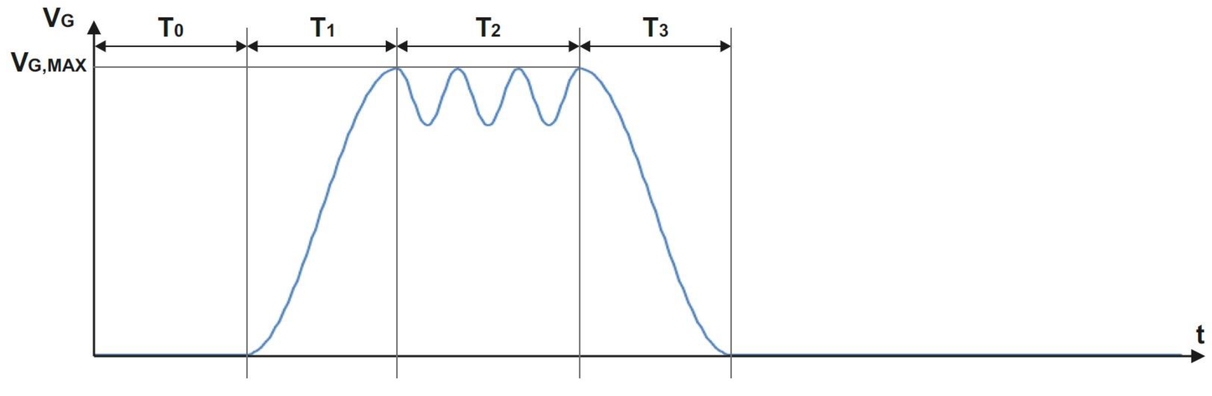
2.3.3. Gust Modeling Method
- Mach number;
- X-component of the flow direction;
- Y-component of flow direction;
- Z-component of flow direction.
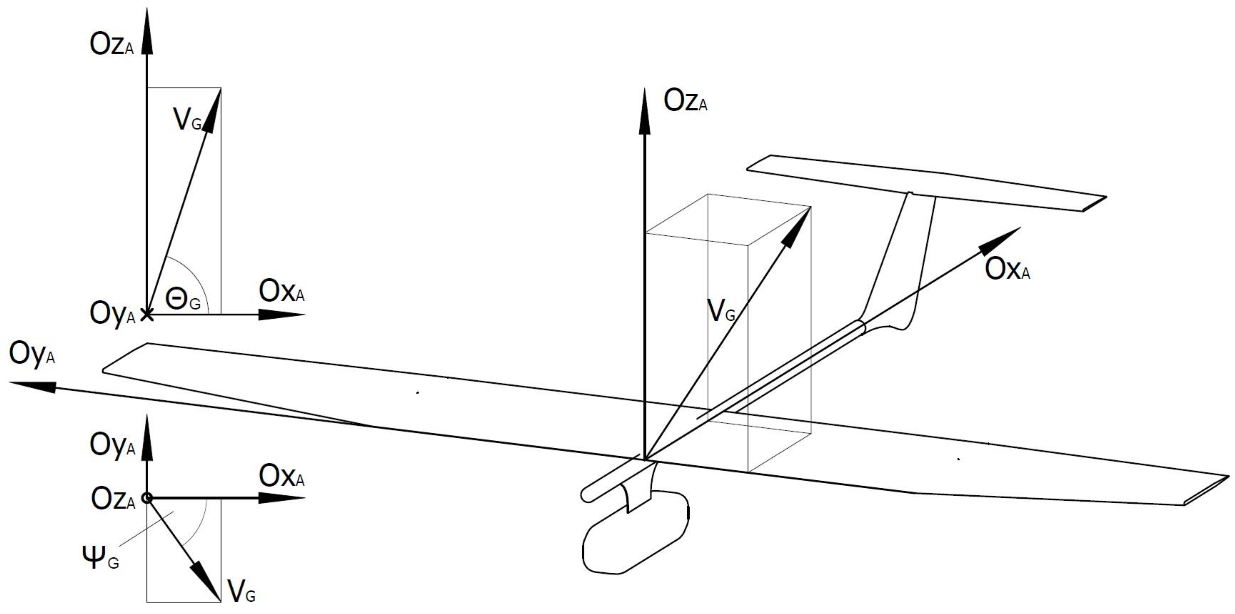
- The OX axis coincides with the longitudinal axis of the studied object and is directed towards its rear;
- The OY axis coincides with the transverse axis and is directed towards the right wing;
- The OZ axis is perpendicular to the OXY plane and directed upwards;
- In the case under analysis, the coordinate system origin was assumed to be at the UAV’s center of gravity.
- The OxA axis was directed correspondingly in the direction of the air streams and parallel to them;
- The OzA axis was directed upwards, perpendicular to the axis OxA and lay in the symmetry plane of the model;
- The OyA axis was directed to the right and perpendicular to the OxA andOzA axes.
3. Results and Discussion
3.1. Numerical Models Validation
3.2. Influence of Gusts on Aerodynamic Characteristics of UAV
- Forces in the OXYZ coordinate system;
- Rolling, pitching and yawing moments (aerodynamic moments were determined relative to the point lying on the leading edge of the wing, in the UAV’s symmetry plane);
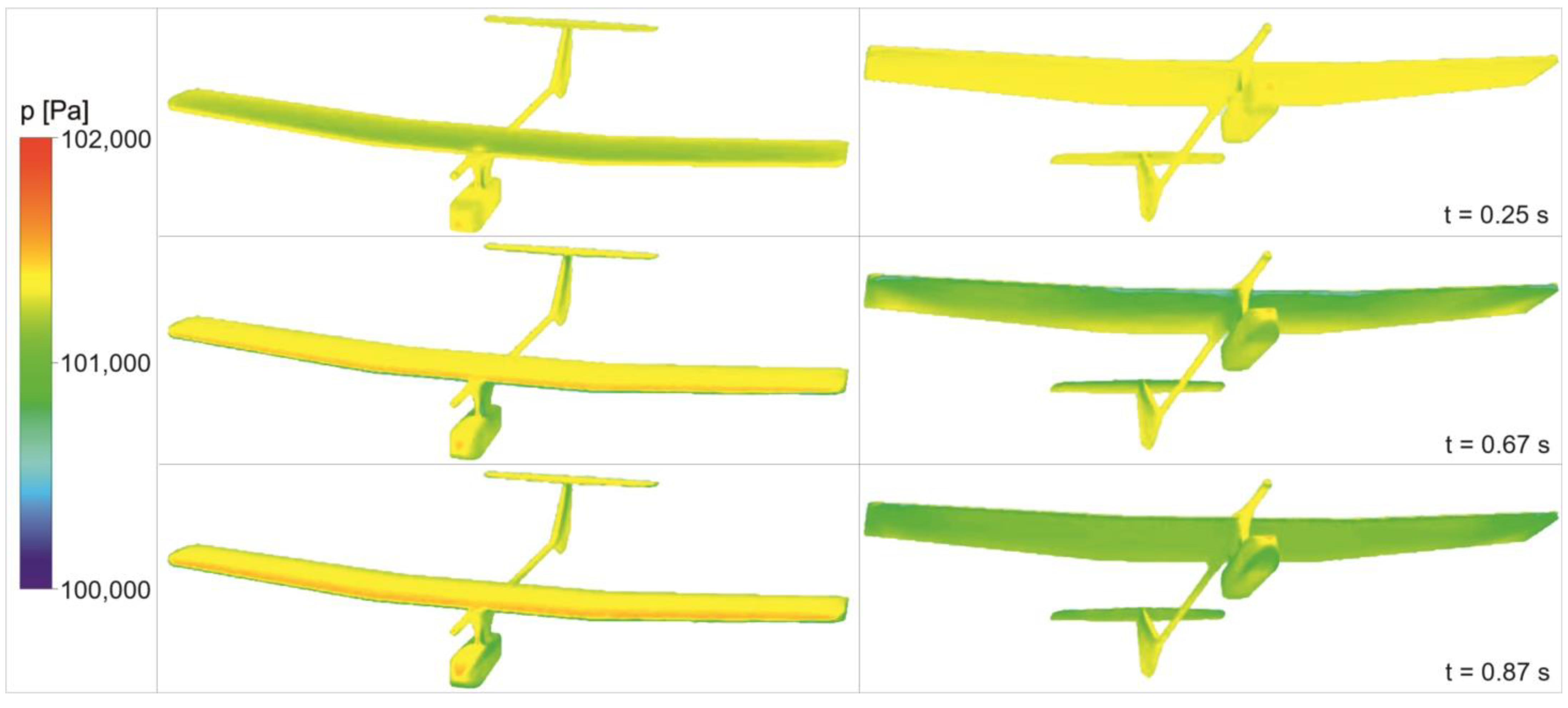
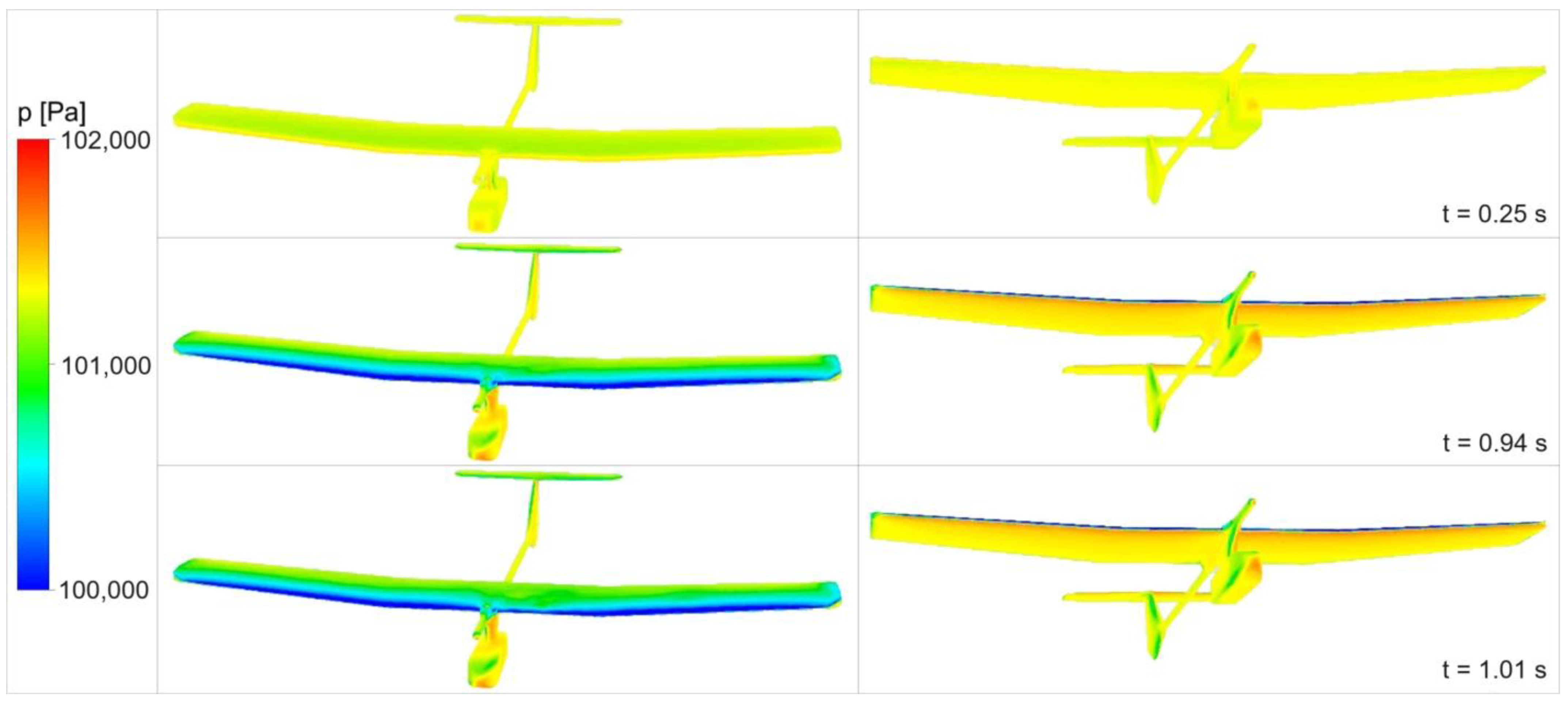
- Contours of static pressure on the UAV’s surfaces.
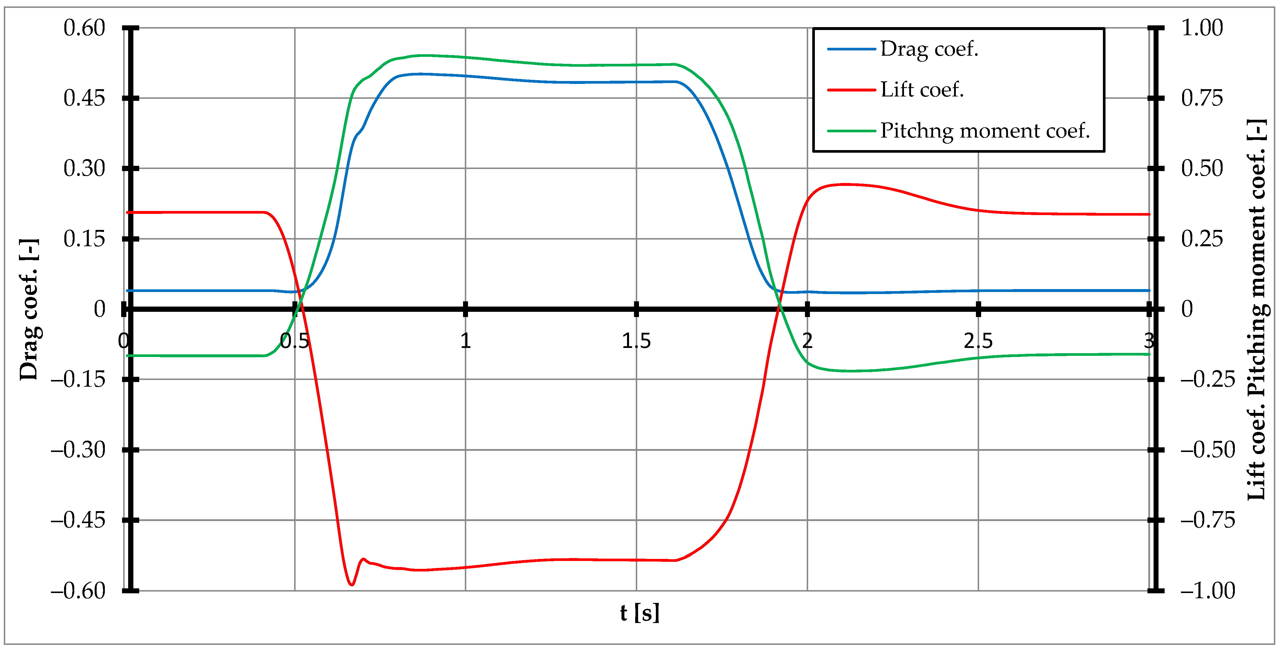
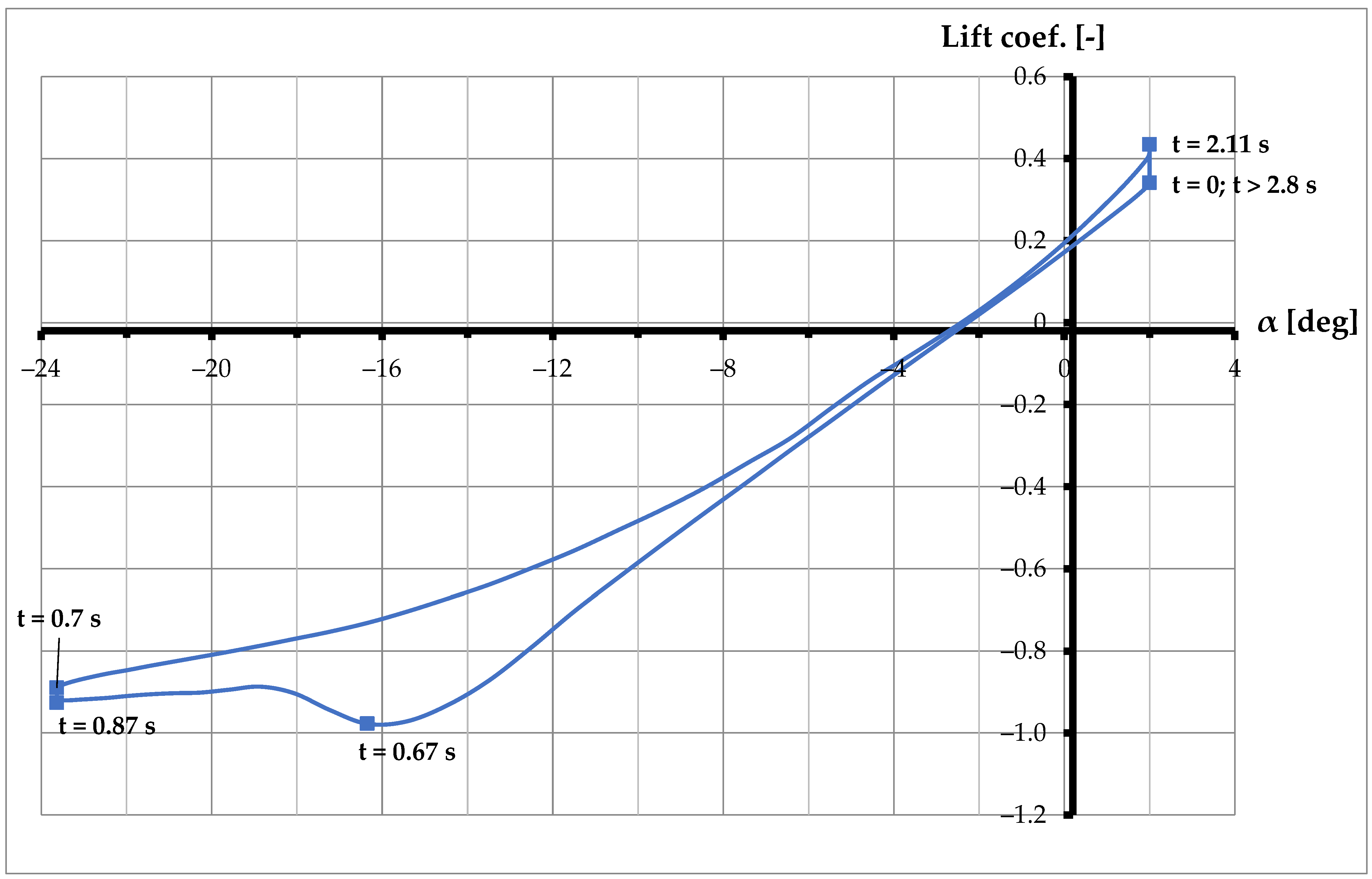
3.2.1. Down Draft
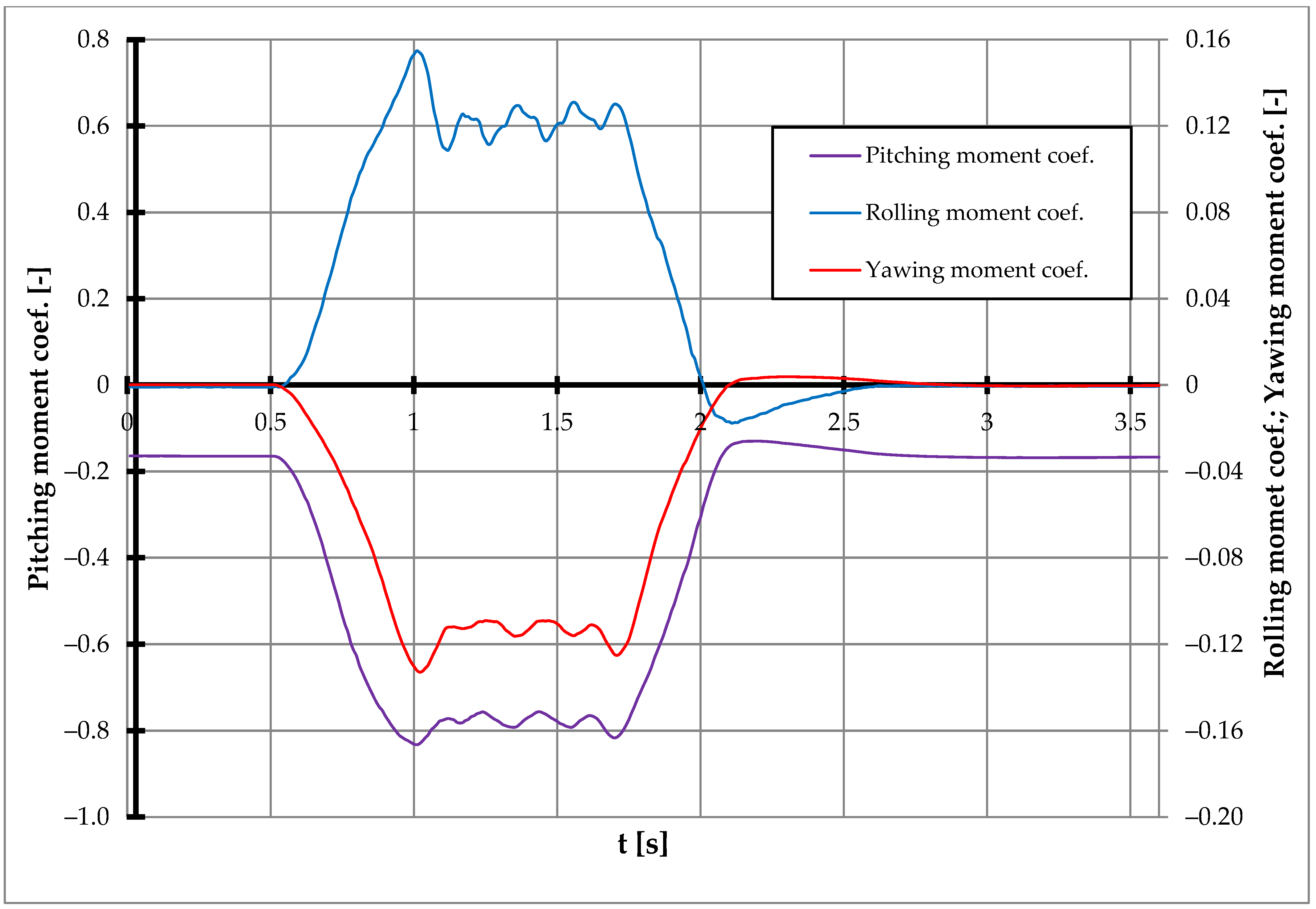
3.2.2. Oblique Gust
4. Conclusions
Author Contributions
Funding
Data Availability Statement
Conflicts of Interest
References
- Bowen, Y.; Pakwai, C.; Qiusheng, L.; Yuncheng, H.; Ying, C.; Zhenru, S.; Yao, C. Characterization of Wind Gusts: A Study Based on Meteorological Tower Observations. Appl. Sci. 2022, 12, 2105. [Google Scholar] [CrossRef]
- Szwed, P.; Rzucidło, P.; Rogalski, T. Estimation of Atmospheric Gusts Using Integrated On-Board Systems of a Jet Transport Airplane—Flight Simulations. Appl. Sci. 2022, 12, 6349. [Google Scholar] [CrossRef]
- Shelekhov, A.; Afanasiev, A.; Shelekhova, E.; Kobzev, A.; Tel’minov, A.; Molchunov, A.; Poplevina, O. High-Resolution Profiling of Atmospheric Turbulence Using UAV Autopilot Data. Drones 2023, 7, 412. [Google Scholar] [CrossRef]
- Li, C.; Tan, H.; Wang, G.; Chan, P.; Luo, Y. Application of a Three-Dimensional Wind Field from a Phased-Array Weather Radar Network in Severe Convection Weather. Atmosphere 2023, 14, 781. [Google Scholar] [CrossRef]
- Zhang, A.; Zhang, S.; Xu, X.; Zhong, H.; Li, B. Variation Characteristics of the Wind Field in a Typical Thunderstorm Event in Beijing. Appl. Sci. 2022, 12, 12036. [Google Scholar] [CrossRef]
- Mohamed, A.; Marino, M.; Watkins, S.; Jaworski, J.; Jones, A. Gusts Encountered by Flying Vehicles in Proximity to Buildings. Drones 2023, 7, 22. [Google Scholar] [CrossRef]
- Aircraft Accident Report NTSB/AAR-86/05; NTSB: Washington, DC, USA, 1986. Available online: https://www.ntsb.gov/investigations/AccidentReports/Reports/AAR8605.pdf (accessed on 25 August 2023).
- Weather-Related Aviation Accident Study 2003–2007; FAA: Washington, DC, USA, 2010. Available online: https://www.asias.faa.gov/i/studies/2003-2007weatherrelatedaviationaccidentstudy.pdf (accessed on 25 August 2023).
- Maślanka, P.; Szafrańska, H.; Aleksieiev, A.; Korycki, R.; Kaziur, P.; Dąbrowska, A. Influence of Material Degradation on Deformation of Paraglider during Flight. Materials 2023, 16, 5396. [Google Scholar] [CrossRef]
- Chodnicki, M.; Siemiatkowska, B.; Stecz, W.; Stępień, S. Energy Efficient UAV Flight Control Method in an Environment with Obstacles and Gusts of Wind. Energies 2022, 15, 3730. [Google Scholar] [CrossRef]
- Jung, C.; Schindler, D.; Buchholz, A.; Liable, J. Global Gust Climate Evaluation and Its Influence on Wind Turbines. Energies 2017, 10, 1474. [Google Scholar] [CrossRef]
- Chiodo, E.; Diban, B.; Mazzanti, G.; De Angelis, F. A Review on Wind Speed Extreme Values Modeling and Bayes Estimation for Wind Power Plant Design and Construction. Energies 2023, 16, 5456. [Google Scholar] [CrossRef]
- Herisanu, N.; Marinca, V.; Madescu, G.; Dragan, F. Dynamic Response of a Permanent Magnet Synchronous Generator to a Wind Gust. Energies 2019, 12, 915. [Google Scholar] [CrossRef]
- Yitao, Z.; Zhigang, W.; Chao, Y. Study of Gust Calculation and Gust Alleviation: Simulations and Wind Tunnel Tests. Aerospace 2023, 10, 139. [Google Scholar] [CrossRef]
- Reiswich, A.; Finster, M.; Heinrich, M.; Schwarze, R. Effect of Flexible Flaps on Lift and Drag of Laminar Profile Flow. Energies 2020, 13, 1077. [Google Scholar] [CrossRef]
- Kotsiopoulou, M.; Bouris, D. Numerical Simulation of the Effect of a Single Gust on the Flow Past a Square Cylinder. Fluids 2022, 7, 303. [Google Scholar] [CrossRef]
- Lakshmi, S.; Nishanth, R.; Sudharshan, B.R.; Unnikrishnan, D.; Akram, M.; Ratna, K.V. Effect of Macroscopic Turbulent Gust on the Aerodynamic Performance of Vertical Axis Wind Turbine. Energies 2023, 16, 2250. [Google Scholar] [CrossRef]
- Santo, G.; Peeters, M.; Van Paepegem, W.; Degroote, J. Fluid–Structure Interaction Simulations of a Wind Gust Impacting on the Blades of a Large Horizontal Axis Wind Turbine. Energies 2020, 13, 509. [Google Scholar] [CrossRef]
- Cai, X.; Pan, P.; Zhu, J.; Gu, R. The Analysis of the Aerodynamic Character and Structural Response of Large-Scale Wind Turbine Blades. Energies 2013, 6, 3134–3148. [Google Scholar] [CrossRef]
- Benaouali, A.; Kachel, S. Multidisciplinary Design Optimization of Aircraft Wing Using Commercial Software Integration. Aerosp. Sci. Technol. 2019, 92, 766–776. [Google Scholar] [CrossRef]
- Kozakiewicz, A.; Frant, M.; Majcher, M. Impact of the Intake Vortex on the Stability of the Turbine Jet Engine Intake System. Int. Rev. Aerosp. Eng. 2021, 14, 173. [Google Scholar] [CrossRef]
- Wu, C.-H.; Chen, J.-Z.; Lo, Y.-L.; Fu, C.-L. Numerical and Experimental Studies on the Aerodynamics of NACA64 and DU40 Airfoils at Low Reynolds Numbers. Appl. Sci. 2023, 13, 1478. [Google Scholar] [CrossRef]
- Frant, M. Numerical Analysis of Complex Objects Aerodynamics Using Finite Volume Methods. Ph.D. Thesis, Military University of Technology, Warsaw, Poland, 2010. [Google Scholar]
- Cravero, C.; De Domenico, D.; Marsano, D. The Use of Uncertainty Quantification and Numerical Optimization to Support the Design and Operation Management of Air-Staging Gas Recirculation Strategies in Glass Furnaces. Fluids 2023, 8, 76. [Google Scholar] [CrossRef]
- Xia, L.; Zou, Z.J.; Wang, Z.H.; Zou, L.; Gao, H. Surrogate model based uncertainty quantification of CFD simulations of the viscous flow around a ship advancing in shallow water. Ocean Eng. 2021, 234, 109206. [Google Scholar] [CrossRef]
- Cravero, C.; De Domenico, D.; Marsano, D. Uncertainty Quantification Analysis of Exhaust Gas Plume in a Crosswind. Energies 2023, 16, 3549. [Google Scholar] [CrossRef]
- Huang, Y.; Guo, X.; Cao, D. Aerodynamic Characteristics of a Z-Shaped Folding Wing. Aerospace 2023, 10, 749. [Google Scholar] [CrossRef]
- Tofan-Negru, A.; Ștefan, A.; Grigore, L.S.; Oncioiu, I. Experimental and Numerical Considerations for the Motor-Propeller Assembly’s Air Flow Field over a Quadcopter’s Arm. Drones 2023, 7, 199. [Google Scholar] [CrossRef]
- Zhang, Z.; Xie, C.; Wang, W.; An, C. An Experimental and Numerical Evaluation of the Aerodynamic Performance of a UAV Propeller Considering Pitch Motion. Drones 2023, 7, 447. [Google Scholar] [CrossRef]
- Ghirardelli, M.; Kral, S.; Müller, N.; Hann, R.; Cheynet, E.; Reuder, J. Flow Structure around a Multicopter Drone: A Computational Fluid Dynamics Analysis for Sensor Placement Considerations. Drones 2023, 7, 467. [Google Scholar] [CrossRef]
- Pérez Gordillo, A.M.; Escobar, J.A.; Lopez Mejia, O.D. Influence of the Reynolds Number on the Aerodynamic Performance of a Small Rotor. Aerospace 2023, 10, 130. [Google Scholar] [CrossRef]
- Lei, Y.; Li, Y.; Wang, J. Aerodynamic Analysis of an Orthogonal Octorotor UAV Considering Horizontal Wind Disturbance. Aerospace 2023, 10, 525. [Google Scholar] [CrossRef]
- ANSYS FLUENT Theory Guide; ANSYS, Inc.: Canonsburg, PA, USA, 2015.
- Krzyżanowski, A. Mechanika Lotu; Wydział Wydawniczy WAT: Warsaw, Poland, 2009. [Google Scholar]
- ANSYS FLUENT UDF Manual; ANSYS, Inc.: Canonsburg, PA, USA, 2015.
- Yousefi, K.; Razeghi, A. Determination of the Critical Reynolds Number for Flow over Symmetric NACA Airfoils. In Proceedings of the 2018 AIAA Aerospace Sciences Meeting, Kissimmee, FL, USA, 8–12 January 2018. [Google Scholar] [CrossRef]
- Skrzypinski, W.; Zahle, F.; Bak, C. Parametric approximation of airfoil aerodynamic coefficients at high angles of attack. In Proceedings of the European Wind Energy Conference & Exhibition 2014, Barcelona, Spain, 10–13 March 2014; Available online: https://backend.orbit.dtu.dk/ws/files/89913457/Parametric_approximation_of_airfoil.pdf (accessed on 25 August 2023).


| Location | Name | Type |
|---|---|---|
| outer surfaces | outer | pressure far-field |
| fuselage of UAV | fuselage | wall |
| wings of UAV | wing | wall |
| horizontal stabilizer of UAV | horizontal_stab | wall |
| vertical stabilizer of UAV | vert_stab | wall |
| Time [s] | α [deg] | Drag Coef. [-] | Lift Coef. [-] | Pitching Moment Coef. [-] |
|---|---|---|---|---|
| 0.4 | 2 | 0.039 | 0.344 | −0.165 |
| 0.49 | 0 | 0.037 (local minimum) | ||
| 0.67 | −16.4 | −0.978 (minimum) | ||
| 0.7 | −18.9 | −0.887 (local maximum) | ||
| 0.87 | −23.6 | 0.501 (maximum) | −0.927 (local minimum) | |
| 0.89 | −23.6 | 0.902 (maximum) | ||
| 1.25 ÷ 1.6 | 23.6 | 0.483 ÷ 0.485 | −0.892 ÷ 0.889 | 0.866 ÷ 0.87 |
| 2.11 | 2 | 0.433 (maximum) | ||
| 2.12 | 2 | 0.0035 (minimum) | ||
| 2.13 | 2 | −0.22 (minimum) |
| Time [s] | α [deg] | β [deg] | Drag Coef. [-] | Side Force Coef. [-] | Lift Coef. [-] | Rolling Moment Coef. [-] | Pitching Moment Coef. [-] | Yawing Moment Coef. [-] |
|---|---|---|---|---|---|---|---|---|
| 0 ÷ 0.5 | 2 | 0 | 0.039 | ca. 0 | 0.344 | ca. 0 | −0.165 | ca. 0 |
| 0.94 | 17.8 | 10.9 | 1.35 max | |||||
| 1.01 | 18.6 | 11.4 | 0.268 max | 0.155 max | −0.833 min | |||
| 1.02 | 18.6 | 11.4 | 0.119 max | −0.133 min | ||||
| 2.11 | 2.02 | 0.02 | −0.018 min | |||||
| 2.18 | 2 | 0 | 0.283 min | |||||
| 2.19 | 2 | 0 | −0.13 max | |||||
| 2.22 | 2 | 0 | −0.003 min | |||||
| 2.3 | 2 | 0 | 0.004 max | |||||
| 3.05 | 2 | 0 | 0.0388 min |
Disclaimer/Publisher’s Note: The statements, opinions and data contained in all publications are solely those of the individual author(s) and contributor(s) and not of MDPI and/or the editor(s). MDPI and/or the editor(s) disclaim responsibility for any injury to people or property resulting from any ideas, methods, instructions or products referred to in the content. |
© 2023 by the authors. Licensee MDPI, Basel, Switzerland. This article is an open access article distributed under the terms and conditions of the Creative Commons Attribution (CC BY) license (https://creativecommons.org/licenses/by/4.0/).
Share and Cite
Frant, M.; Kachel, S.; Maślanka, W. Gust Modeling with State-of-the-Art Computational Fluid Dynamics (CFD) Software and Its Influence on the Aerodynamic Characteristics of an Unmanned Aerial Vehicle. Energies 2023, 16, 6847. https://doi.org/10.3390/en16196847
Frant M, Kachel S, Maślanka W. Gust Modeling with State-of-the-Art Computational Fluid Dynamics (CFD) Software and Its Influence on the Aerodynamic Characteristics of an Unmanned Aerial Vehicle. Energies. 2023; 16(19):6847. https://doi.org/10.3390/en16196847
Chicago/Turabian StyleFrant, Michał, Stanisław Kachel, and Wojciech Maślanka. 2023. "Gust Modeling with State-of-the-Art Computational Fluid Dynamics (CFD) Software and Its Influence on the Aerodynamic Characteristics of an Unmanned Aerial Vehicle" Energies 16, no. 19: 6847. https://doi.org/10.3390/en16196847
APA StyleFrant, M., Kachel, S., & Maślanka, W. (2023). Gust Modeling with State-of-the-Art Computational Fluid Dynamics (CFD) Software and Its Influence on the Aerodynamic Characteristics of an Unmanned Aerial Vehicle. Energies, 16(19), 6847. https://doi.org/10.3390/en16196847