Numerical Simulation of the Effects of Blade–Arm Connection Gap on Vertical–Axis Wind Turbine Performance

Abstract

Many vertical-axis wind turbines (VAWTs) require arms, which generally provide aerodynamic resistance, to connect the main blades to the rotating shaft. Three–dimensional numerical simulations were conducted to clarify the effects of a gap placed at the blade–arm connection portion on VAWT performance. A VAWT with two straight blades (diameter: 0.75 m, height: 0.5 m) was used as the calculation model. Two horizontal arms were assumed to be connected to the blade of the model with or without a gap. A cylindrical rod with a diameter of 1 or 5 mm was installed in the gap, and its length varied from 10 to 30 mm. The arm cross section has the same airfoil shape (NACA 0018) as the main blade; however, the chord length is half (0.04 m) that of the blade. The simulation shows that the power of the VAWT with gaps is higher than that of the gapless VAWT. The longer gap length tends to decrease the power, and increasing the diameter of the connecting rod amplifies this decreasing tendency. Providing a short gap at the blade–arm connection and decreasing the cross–sectional area of the connecting member is effective in increasing VAWT power.

1. Introduction

Most of the wind turbines currently used for wind power generation are propeller–type horizontal–axis wind turbines (HAWTs) [1,2]. A different wind turbine rotor structure is the vertical–axis wind turbine (VAWT) [3,4,5], which has features such as having no wind direction dependence. Unlike HAWTs, many lift–driven VAWTs (Darrieus type) structurally require arms (or struts) to connect the main blades to the rotating shaft. If the cross section of the arm is airfoil–shaped, the slant–installed arm generates a rotational force using lift, which improves the starting performance. However, it becomes the main cause of aerodynamic resistance in a high–rotation–speed state, regardless of the cross section, when installed horizontally. Several previous studies have investigated the effects of arms on the performance of lift–type VAWTs.

Li and Calisal [6] investigated the three–dimensional (3D) effects of a vertical–axis tidal turbine, but not wind turbines, through numerical analysis using the vortex method. However, their numerical simulation did not include the effects of the arm, which were analytically modeled based on separate towing experiments. In their research, two types of arm structures (types A and B) were analyzed. In type B, the arm with the airfoil section was directly connected to the blade. Conversely, in type A, the arm had a bluff body–shaped cross section, which was attached to the blade via a clamping mechanism to adjust the angle of attack. As a result, type A caused larger arm loss than type B.

Qin et al. [7] conducted a computational fluid dynamics (CFD) analysis based on the Reynolds–averaged Navier–Stokes (RANS) equations of an H–type VAWT with a rooftop (diameter: 2.5 m, blade length: 2 m, chord length: c = 0.2 m) consisting of three blades. The 3D model was equipped with a flat cylindrical rotor hub (top disk) with a diameter of 0.5 m. Although the cross–sectional shape of the arm is unknown, the length of the arm connecting the top disk and a blade was set to 1 m. A comparison of the 2D and 3D calculation results showed that the average torque decreased by 40% because of the 3D effects. The authors considered that the observed negative torque, which is larger downstream than upstream, must be attributed to the interaction between the wake generated by the blade passing upwind half and the blade downstream. In Figure 14(a) of their paper, the vorticity generated from the arms was visualized to demonstrate its significant effects. However, the azimuth dependency of the arm effects and the importance of the connection part were not mentioned.

De Marco et al. [8] conducted a CFD analysis on the characteristics of a straight–bladed VAWT (diameter: 2.6 m, blade length: 2.5 m, blade chord length: 20 mm, blade cross section: NACA 0018) equipped with slant arms. The cross–sectional shape of the upper and lower slant arms mounted at 30 degrees on a horizontal arm placed on the equatorial plane was similar to the main blade. The torque generated by the horizontal arms was not considered in the CFD analysis. Three cases in which the number of blades changed from one to three were examined, and in each case, models of the main blade only, arm set only, and full element (both main blades and arms) were calculated. In each case, the full–element characteristics were shown to be inferior to the simple sum of the blade–only and arm set–only models, and the complex effects of wake and blockage with an increasing number of blades were discussed. Figure 14(b) of their paper showed the improvement in rotor power when the chord length of the slant blade was reduced. However, their slant arms were directly attached to the blades, and the effects of the connection portion on the turbine rotor were not mentioned.

Marsh et al. [9] performed an unsteady RANS (URANS) analysis on a vertical–axis tidal current turbine with three straight blades (radius: 0.457 m, blade length: 0.686 m, blade chord length: 65 mm, blade cross section: NACA 0012) using k–ω SST as the turbulence model. Three types of turbines were analyzed. Turbine A was equipped with horizontal struts (section NACA 0012) directly connected to the blade tips (upper and lower). The other two turbines (turbines B and C) were structured with a horizontal strut attached to the quarter position of the blade length from each upper and lower blade tip. The cross section of the strut of turbine B had a bluff body shape, and the strut was connected to a blade with a connection tab. In contrast, the strut section of turbine C was airfoil–shaped (NACA 0012), and the strut was directly connected to the blade (faired joint). Turbine A clearly showed a smaller power coefficient (C_p) than turbines B and C. Turbine B generated a smaller rotational torque than turbine C; however, it is not clear whether the shape of the strut or the connecting tab had a greater effect, with the authors stating that the distinction is difficult to determine.

Li et al. [10] conducted a wind tunnel experiment using an experimental rotor with a diameter, blade length, and chord length of 20 m, 1.2 m, and 0.265 m, respectively, to clarify the aerodynamic characteristics of a straight–blade VAWT. The cross section of the main blade was NACA 0021. The number of blades was changed from two to five to investigate the effects of solidity and Reynolds number. The shapes of the arms were not described in detail. In addition to pressure measurements using 32 pressure taps at the mid–span cross section of the blade, torque meter measurements and six–component force balance measurements were performed. The C_p obtained by the pressure measurement was larger than the C_p measured by the torque meter or force balance. This difference was attributed to the fact that the pressure measurement did not include the blade tip or arm effects. Their study also presented CFD results showing the azimuth dependence of the torque at different positions in the span direction of one blade. The results illustrated that at the upstream position (azimuth 90°), where the maximum torque was generated, the torque generated near the equatorial level was approximately 40% higher than that near the blade tip.

Aihara et al. [11] performed 3D–CFD (RANS, turbulence model: realizable k–ε) on a 12 kW three–bladed VAWT with a diameter and blade length of 6.5 m and 5 m, respectively. The azimuth dependency of the normal and tangential forces of one blade and one inclined strut (upper and lower) was calculated for three cases: blade only, with strut, and with tower. The C_p for the blade–only model was 0.277 and that with struts decreased by 43% to become 0.158. The influence of the tower was smaller than that of the struts. The tangential force was more strongly influenced by the strut than the normal force and decreased at the height of the connection between the strut and the blade. Furthermore, at 90° azimuth (upstream), the reduction in the tangential force owing to the struts was large. Note that there was no gap between the strut and the blade in their model.

In most vertical–axis turbines actually installed in the field, such as the aforementioned 12 kW VAWT, an arm and a blade are directly connected without creating any gap or changing the cross–sectional area of the arm (see Figure 1 of reference [12] and the conceptual video or images shown in the web page [13]).

Hara et al. [14] performed a CFD analysis to elucidate the effects of the arms on the performance of a VAWT. The analysis objects (diameter: 0.75 m, blade length: 0.5 m, blade chord length: 80 mm, blade cross section: NACA 0018) consisted of two straight blades without arms (armless rotor) or those with arms having three different cross sections (airfoil, rectangular, and circular). The study showed that the model with airfoil cross–sectional arms reduced the power by approximately 50% under the maximum power condition (tip speed ratio: λ = 3) compared to the model without arms. The drag caused by the surface pressure of the arm tended to increase near the connection between the arm and blade, regardless of the arm cross–sectional shape. Importantly, the rotational force caused by the pressure distribution on the main blade was significantly affected by the arm mounting portion, and the influence largely depended on the cross–sectional area of the arm, that is, the contacting area between the arm and the blade. In this study, the main blade and arm were connected without a gap.

The present study targeted a VAWT model of the same size as that used in a previous study [14]. However, a gap was placed between the main blade and arm to investigate the effects of the connection portion on the rotor performance. In addition, the effects of the gap length and the size of the connecting members installed in the gap were clarified.

2. Methods

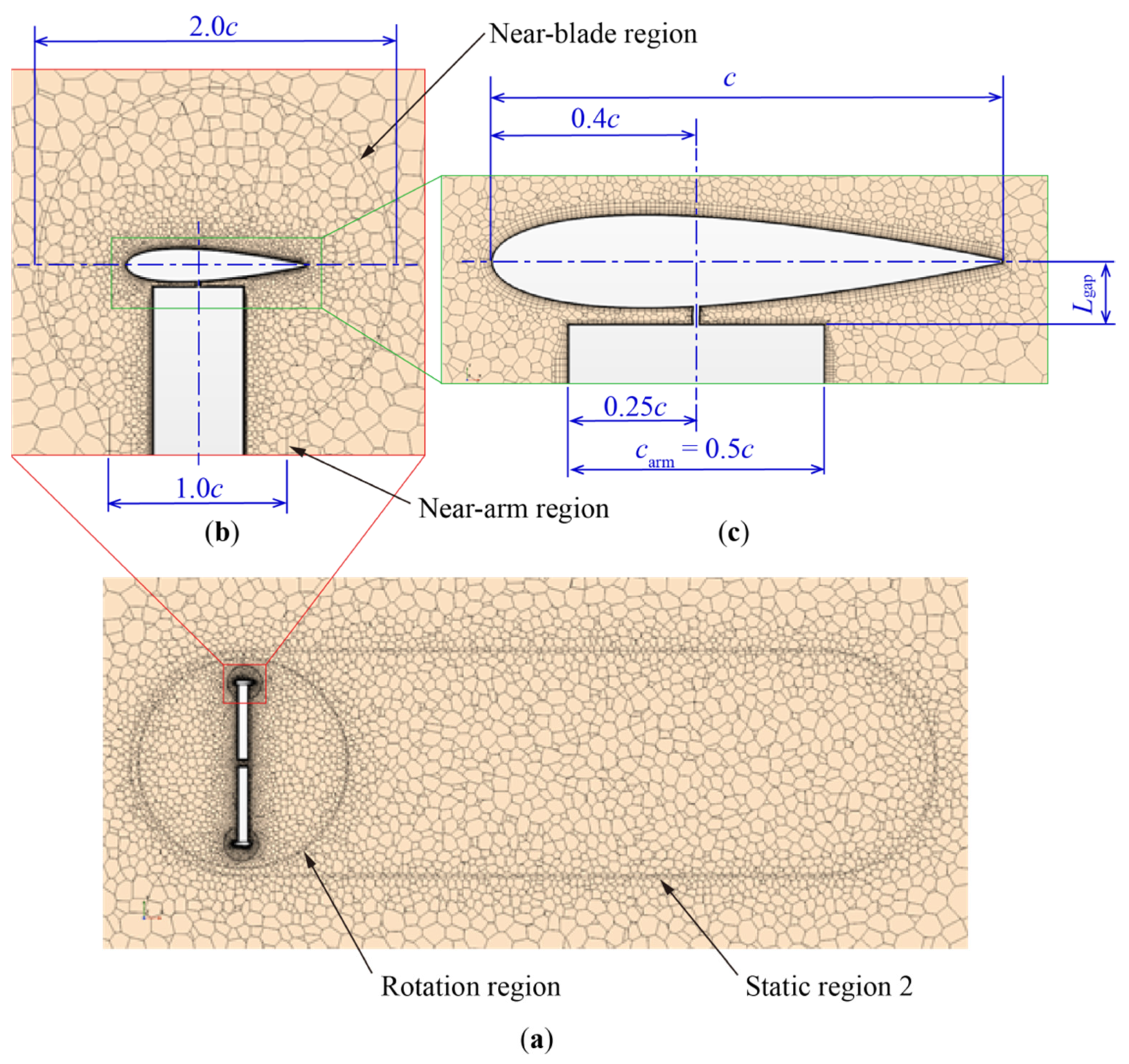
2.1. Object Model for Calculation

Similarly to a previous study [14], a two–bladed H–type Darrieus wind turbine was selected as the calculation object, which had the same size as the experimental VAWT (DU–H2–5075) [15] at the Delft University of Technology (TU Delft) (Figure 1). The cross section of the straight blade (main blade) is NACA 0018 (symmetrical airfoil), with chord length c = 0.08 m, rotor diameter D or 2R = 0.75 m, and blade span 2H = 0.5 m. The blade–mounting position is 40%c (0.032 m). The computational model did not consider the hub or the rotating shaft (or tower) of the wind turbine rotor. Two arms were attached horizontally to each of the main blades, and the arm–mounting position was at one–quarter of the blade span from the top and bottom tips of the main blade. The cross–sectional shape of the arm is NACA 0018, and the chord length of the arm cross section is c_arm = 0.04 m. However, in this research, a gap is put in between the arm and the main blade. Three gap lengths—L_gap = 10 mm, 20 mm, and 30 mm—were assumed for comparison. A model without the gap (gapless), corresponding to the case of L_gap = 0 mm, was analyzed in addition to the other opposite extreme–case model (i.e., armless rotor) that corresponds to L_gap = ∞. In this study, the gap length was defined as the distance between the neutral line of the blade cross section and the outer end of the arm, as shown in Figure 1b. The inner end of the arm is r_root = 20 mm away from the rotor center, and the arm length L_arm varies between 355 mm and 325 mm depending on the gap length. A cylindrical rod with a diameter of d = 1 mm or 5 mm was installed in the gap as a member connecting the main blade and the arm.

Table 1. Calculation cases (model number and specification).

Model No.	0	1	2	3	4	5	6	7
Lgap	0	10	20	30	10	20	30	∞
Larm	355	345	335	325	345	335	325	0
d	-	1	1	1	5	5	5	-

summarizes the calculation cases, that is, the specifications of each model. In the present CFD analysis, the upstream wind speed was set to U_∞ = 7 m/s, and the tip speed ratio was set to λ or Rω/U_∞ = 3.0, which almost matches the maximum C_p state of the object turbine. Therefore, the rotation speed of the wind turbine was set to 535 rpm. The Reynolds number based on the chord length c is Re = 1.1 × 10⁵. Figure 1 also shows an absolute coordinate system (x–y–z) with the origin at the center of the rotor. The wind turbine is assumed to begin the rotation from the azimuth origin (ψ = 0), defined as the positive y–axis direction, and rotate counterclockwise as viewed from above.

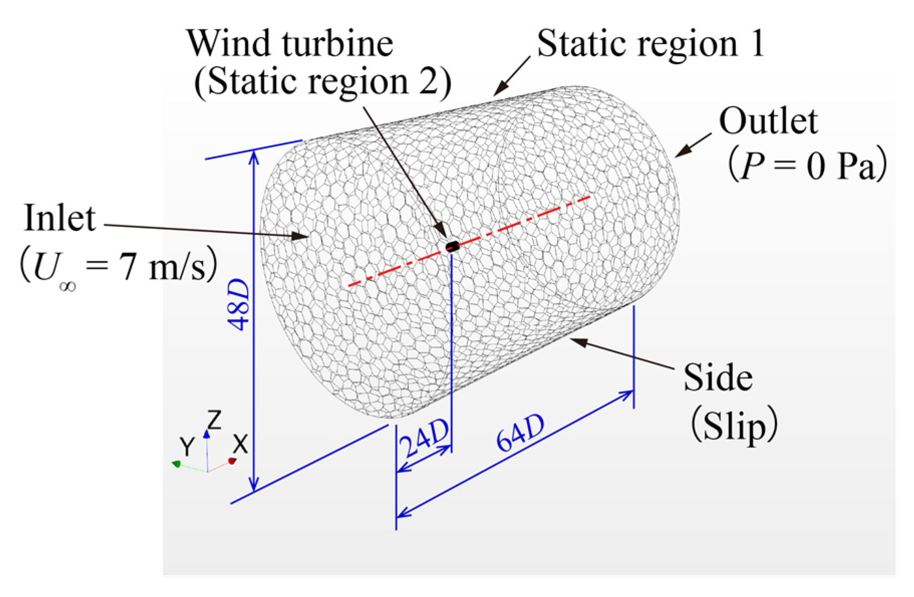
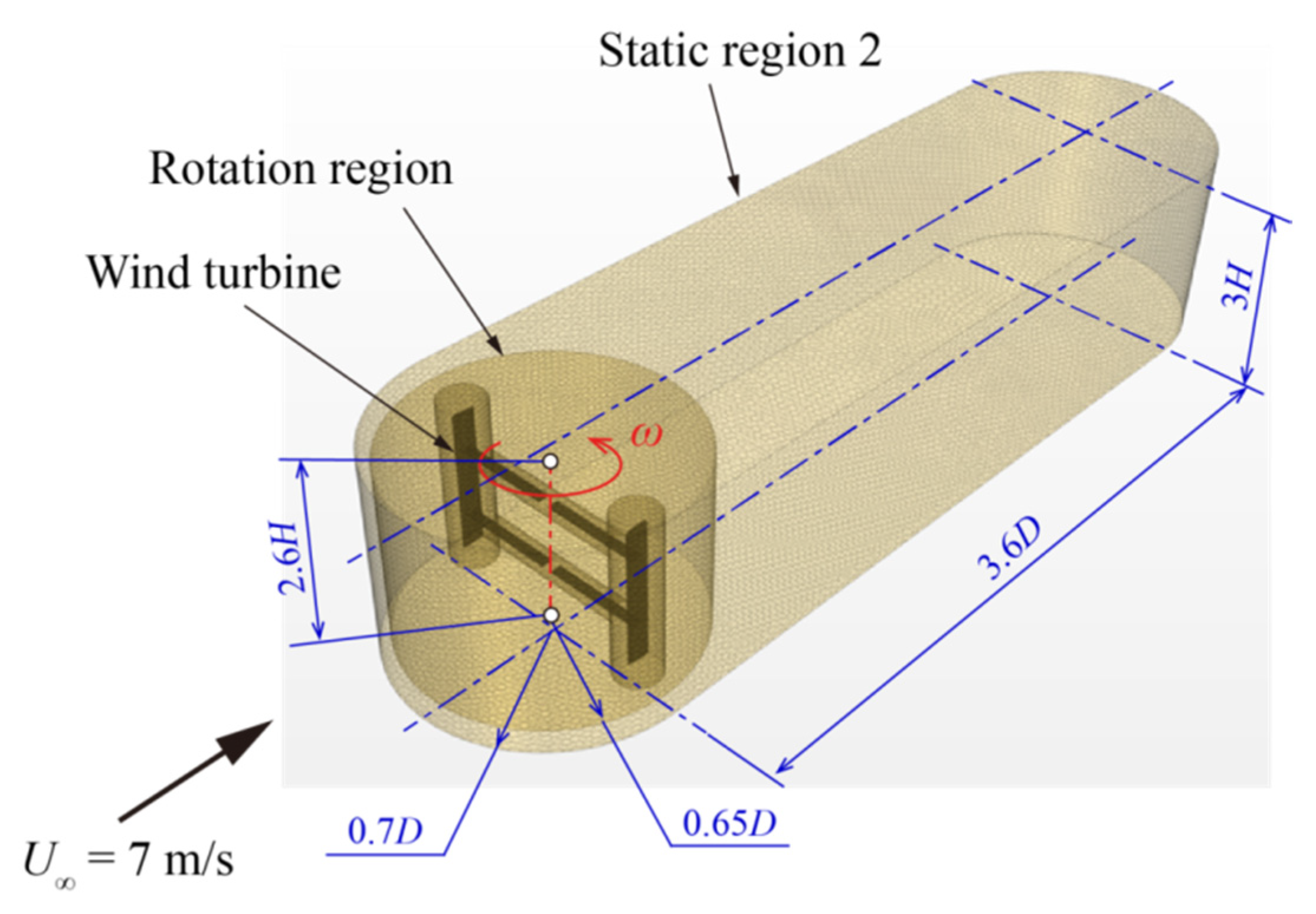
2.2. Settings of Numerical Analysis

STAR–CCM+ was used as the computational solver, and the 3D unsteady incompressible Reynolds–averaged Navier–Stokes (URANS) and continuity equations were used as the basic equations that were solved according to the SIMPLE algorithm. The space discretization procedure was the finite volume method, in which the second–order upwind difference scheme was used. The SST k–ω model [16] was adopted as the turbulence model. The entire computational domain was set as a cylinder with a diameter of 48D and a length of 64D (static region 1), and the center of the wind turbine model was placed at a position 24D from the inlet boundary (see Figure 2). The upstream and downstream boundaries of static region 1 were defined as constant wind speed (U_∞ = 7 m/s) and constant pressure (P = 0 Pa), respectively. A slip condition was applied to the side surface. Figure 3 illustrates the mesh around the wind turbine rotor. The entire rotor was placed in a cylindrical region (rotation region) with a diameter of 1.3D, and this region was moved using the sliding mesh method to provide rotational motion. To adjust the mesh size of the wake region to a nearly constant size, static region 2 was set, which consisted of two semi–cylinders with a radius of 0.7D and a rectangular with a length of 3.6D and a height of 3H. To gradually reduce the mesh size in the region approaching the object surface, a blade was surrounded by a cylindrical region (near–blade region) with a diameter of 2.0c, and an arm was surrounded by another cylindrical region (near–arm region) with a diameter of 1.0c (see Figure 4). An unstructured polyhedral mesh was adopted in most of the computational domain, and a 15–layer prism layer mesh was applied to the region where the boundary layer developed near the object. The minimum grid width was 2.3 × 10⁻⁶ m (blade surface), and the maximum y⁺ was approximately 0.5. The number of cells in the static region is approximately 160,000 (common for all cases), whereas that in the rotation region is approximately 6.34 million and 3.57 million in the case of the gapless and armless rotors, respectively (total number of cells: approximately 6.5 million with arm and 3.7 million without arm). When there was a gap, the number of cells in the rotation region decreased at a rate of approximately 50,000/10 mm–gap. The time interval was 1.56 × 10⁻⁴ s, and the rotor rotated 0.5° per unit time step. Calculations were performed for up to eight revolutions, during which the calculated results, such as the torque, almost converged. The power coefficient was calculated from the average of the seventh rotation, and images were extracted at the eighth rotation. Although the mesh condition is slightly different from that in previous research [14], the calculation region and conditions of the numerical analysis in this research are almost similar to those in the previous research. The azimuth dependence of the one–blade torque of the armless rotor agrees approximately with the results of previous studies. Figure A1 in the Appendix A shows a comparison of the azimuth dependence of the torque coefficient. There is a slight difference at approximately 180°; however, at the other azimuth angles, the present and previous results [14] are almost the same. In addition, the present power coefficient of the rotor with arms at λ = 3 was C_p = 0.0995, which is approximately 21% smaller than the experimental value of C_p = 0.126 at TU Delft [17]. However, the details of the arm shape of the experimental turbine at TU Delft are unknown. The authors claim that this discrepancy is not an essential issue.

3. Results and Discussion

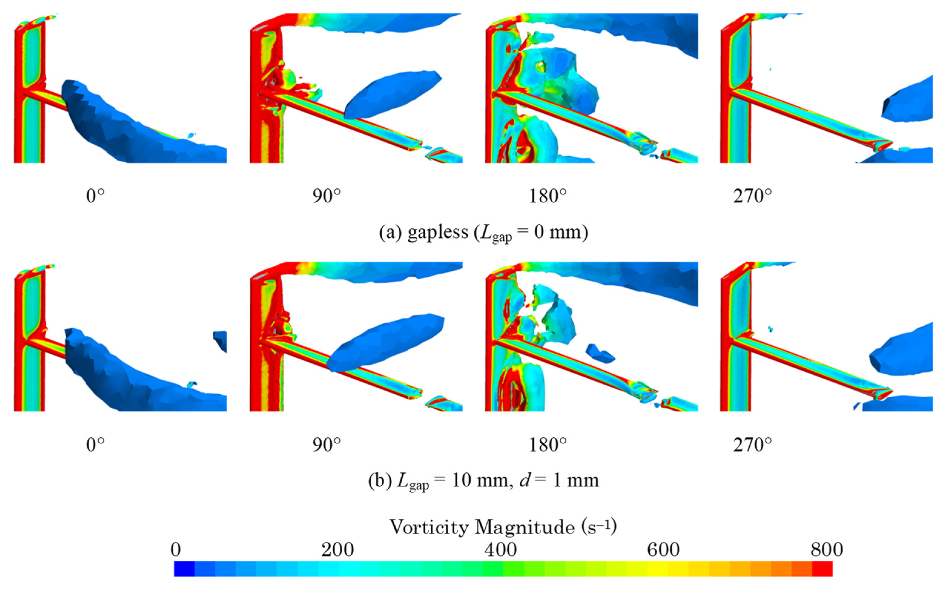
3.1. Vortex Shedding from the Connection Part

To investigate the flow–field state near the connection between the blade and the arm, the Q–criterion isosurfaces [18] (Q = 1000 s⁻²) of model 0 (gapless rotor) and model 1 (L_gap = 10 mm, d = 1 mm) are shown in Figure 5a,b, respectively. The colors represent the strength of the vorticity on the Q–criterion isosurfaces. Figure 5 shows the conditions under which blade 1 of each rotor model is at azimuth angles ψ = 0°, 90°, 180°, and 270° for the two models. For both models, vortex shedding from the connection portion is evident for azimuth angles ψ = 90° and 180°; in particular, the shed vortex is large at the 180° position, where the blade enters from the upwind half to the downwind half. Furthermore, compared with model 1 with a gap, the vortices generated from the connection part in model 0 (gapless), in which the blade and arm are directly connected, appear to affect a wider area of the main blade above and below the connection.

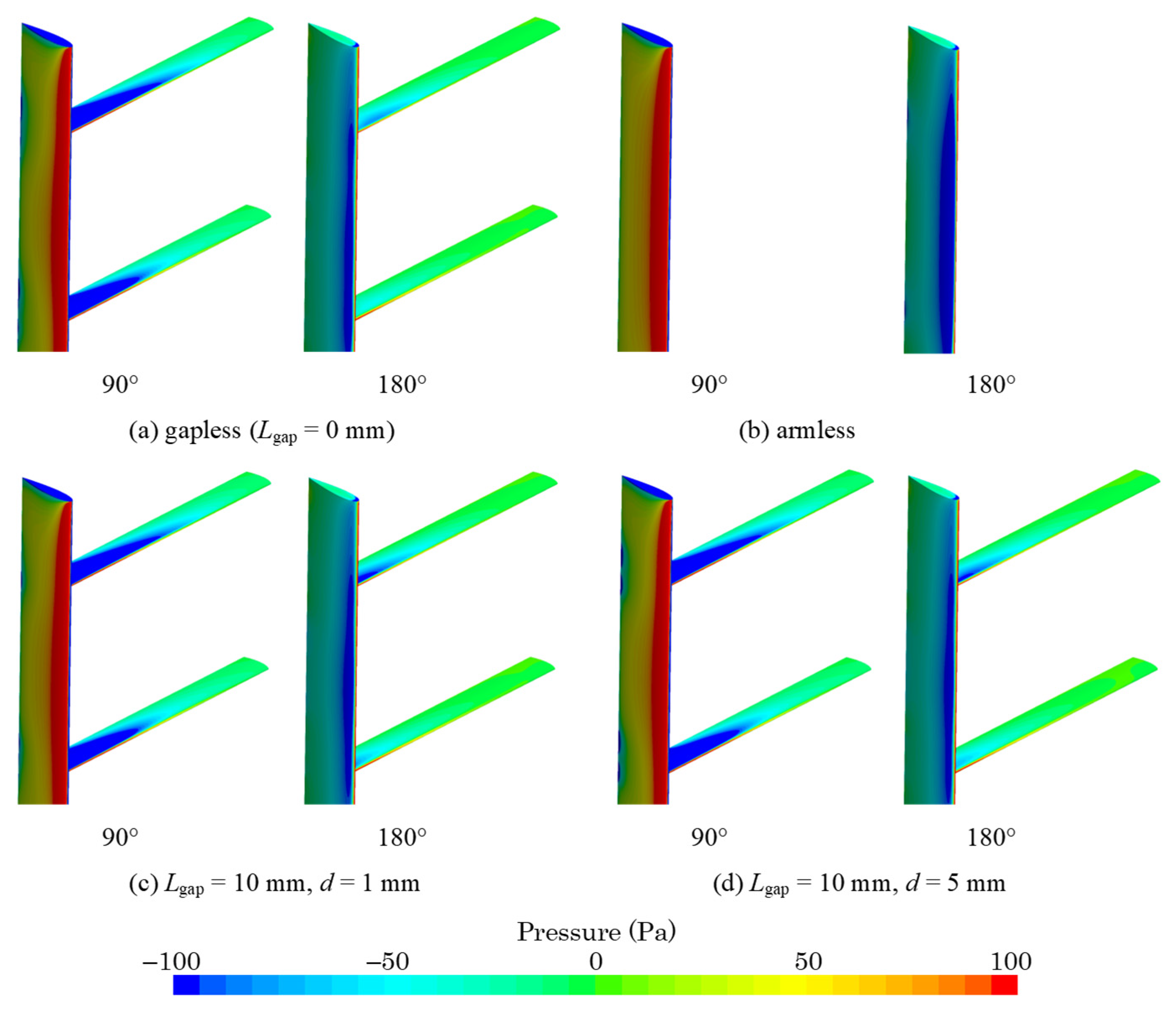
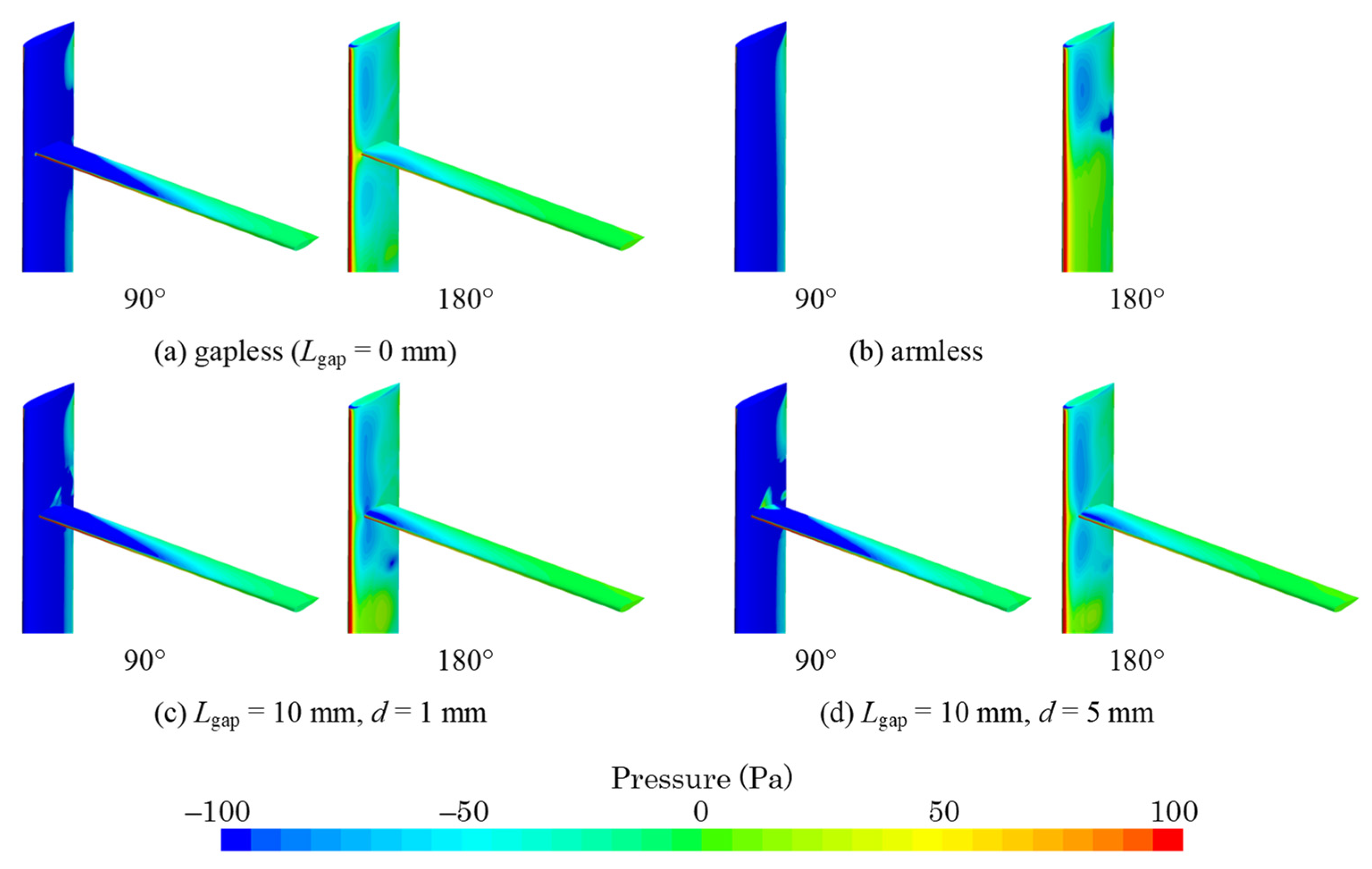
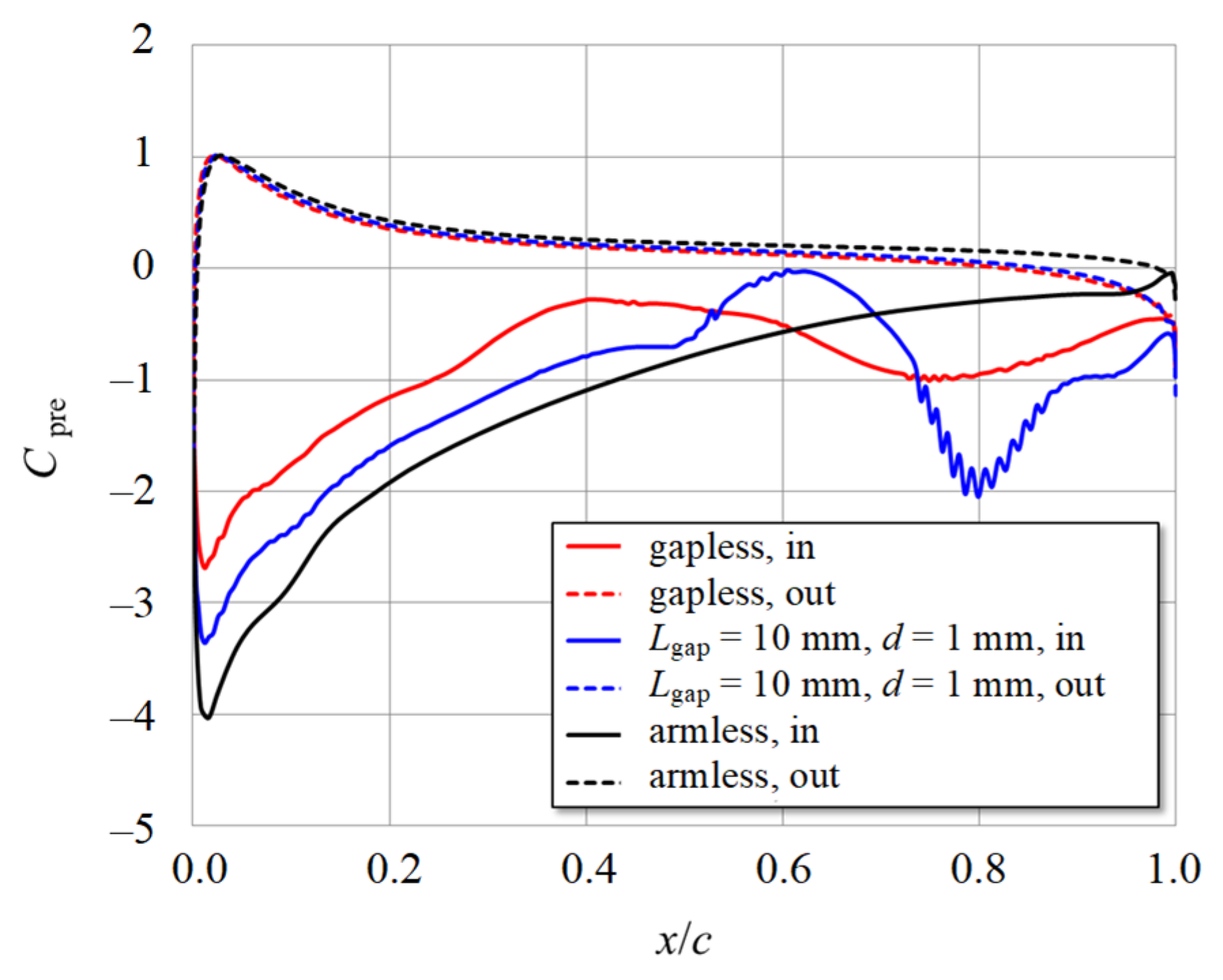
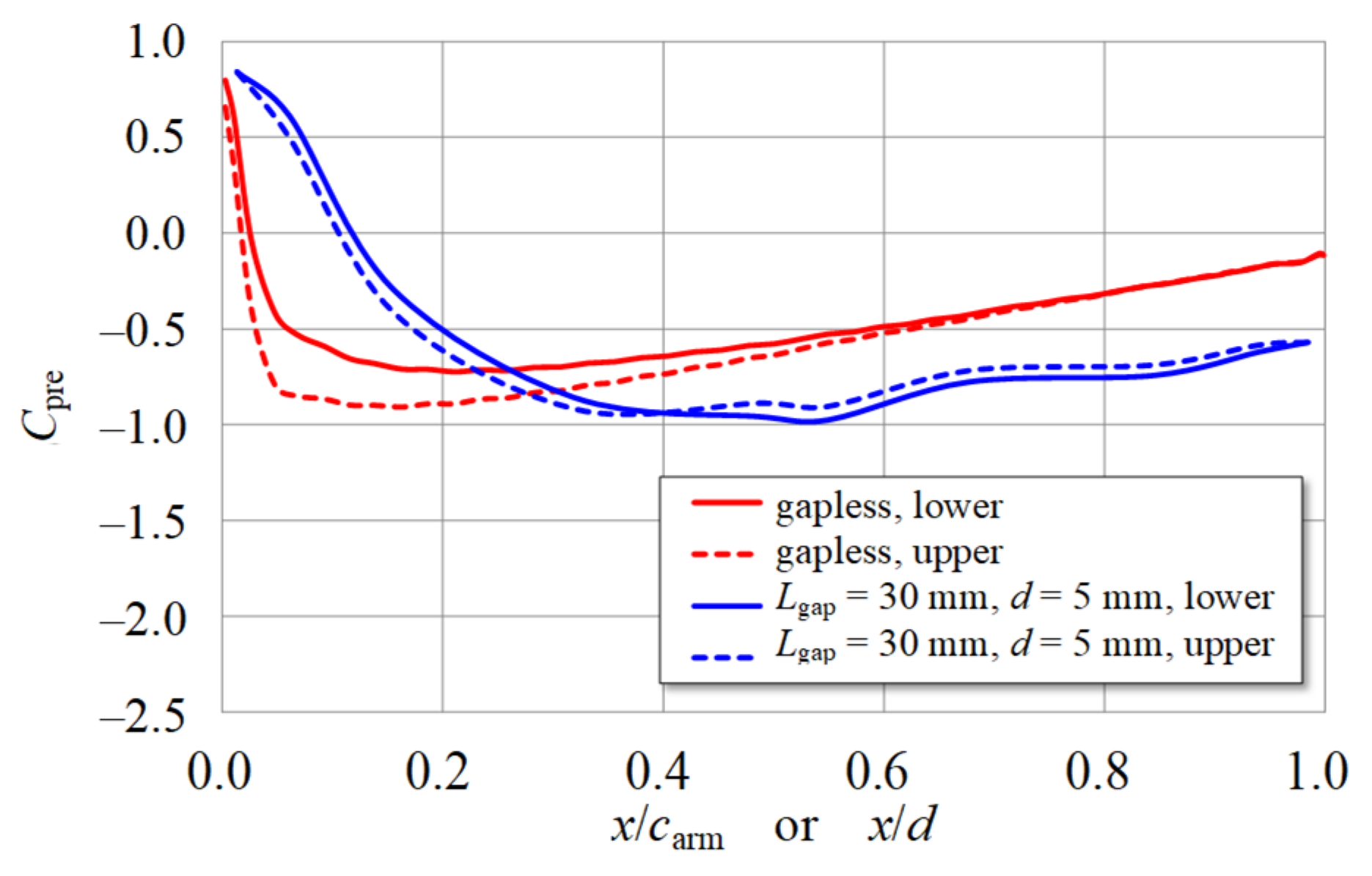
3.2. Surface Pressure Distribution around the Connection Part

Figure 6 shows the surface pressure distribution in the vicinity of the connection part of each blade 1 in the four–rotor models, i.e., model 0 (gapless), model 7 (armless), model 1 (L_gap = 10 mm, d = 1 mm), and model 4 (L_gap = 10 mm, d = 5 mm). The states of azimuth angles ψ = 90° and 180° are shown for each model in this figure. The surface pressure distribution of model 7 (armless) in Figure 6b is clearly different from that of the other rotors with arms. In the pressure distribution of azimuth ψ = 90° in model 7, the inner surface (rotating shaft side) of the blade is entirely negative pressure (blue) to demonstrate that this surface becomes the suction side in the upstream region. The pressure near the trailing edge of the main blade is slightly higher (light blue), except in the vicinity of the blade tip. By contrast, in the other three models with arms, the pressure increase near the trailing edge of the main blade at the azimuth ψ = 90° is suppressed around the arm–blade connection part. In particular, the suppressed area in model 0 (gapless) is wide. As shown in the pressure distribution at ψ = 180° of model 7 (armless), the pressure near the center (equator level) of the blade span is high to indicate that the inner surface of the blade has already switched from the suction side to the pressure side. However, a negative pressure area is observed near the tip of the blade, which is presumed to be due to the influence of the blade tip; however, the cause is not clear. The surface pressure distributions at azimuth ψ = 180° for the other three models with arms are roughly similar. However, unlike models 1 and 4 with gaps, a spot showing rather large positive pressure (yellow area) exists on the main blade in front of the connection portion for the pressure distribution at ψ = 180° of model 0 (gapless rotor).

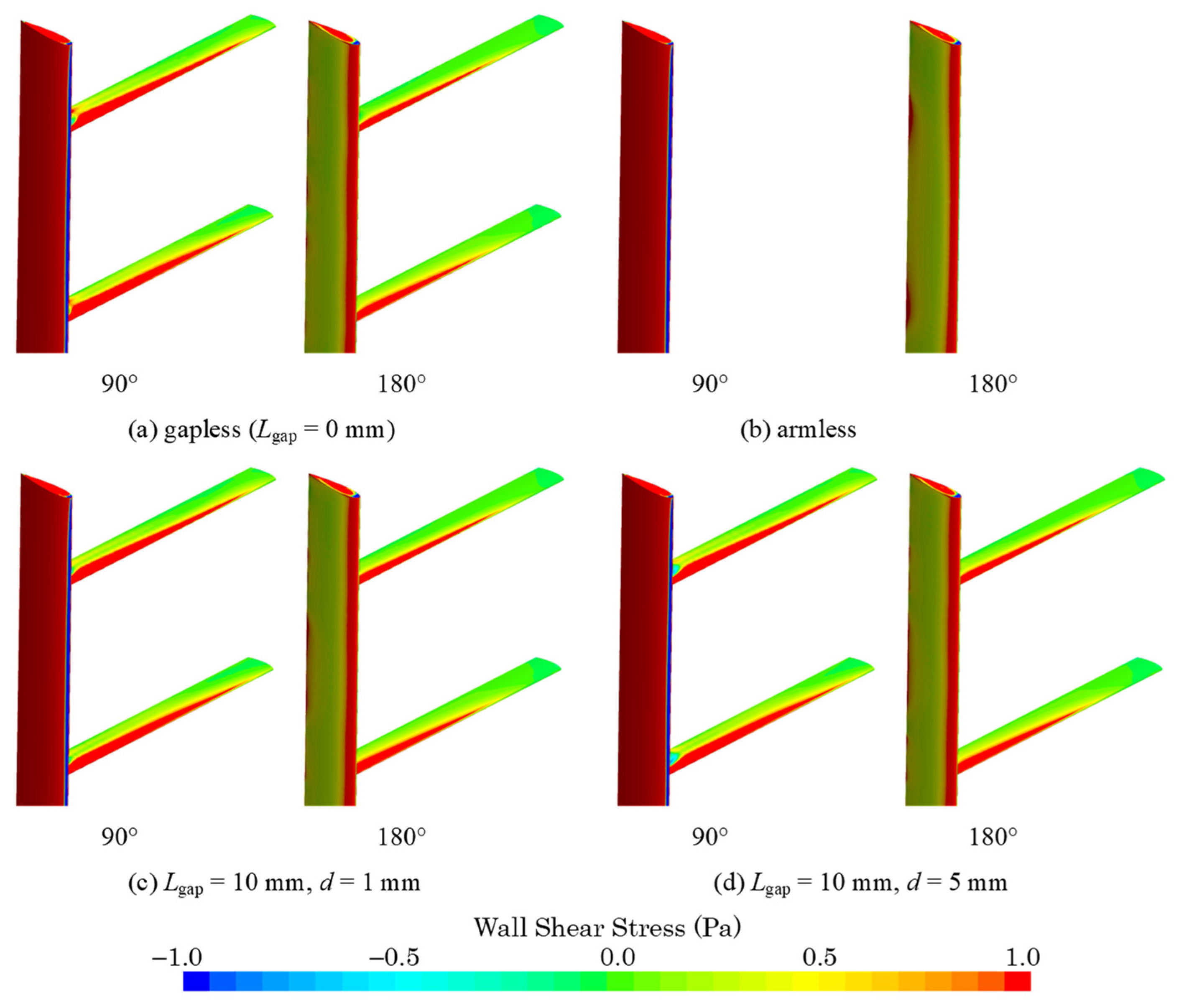
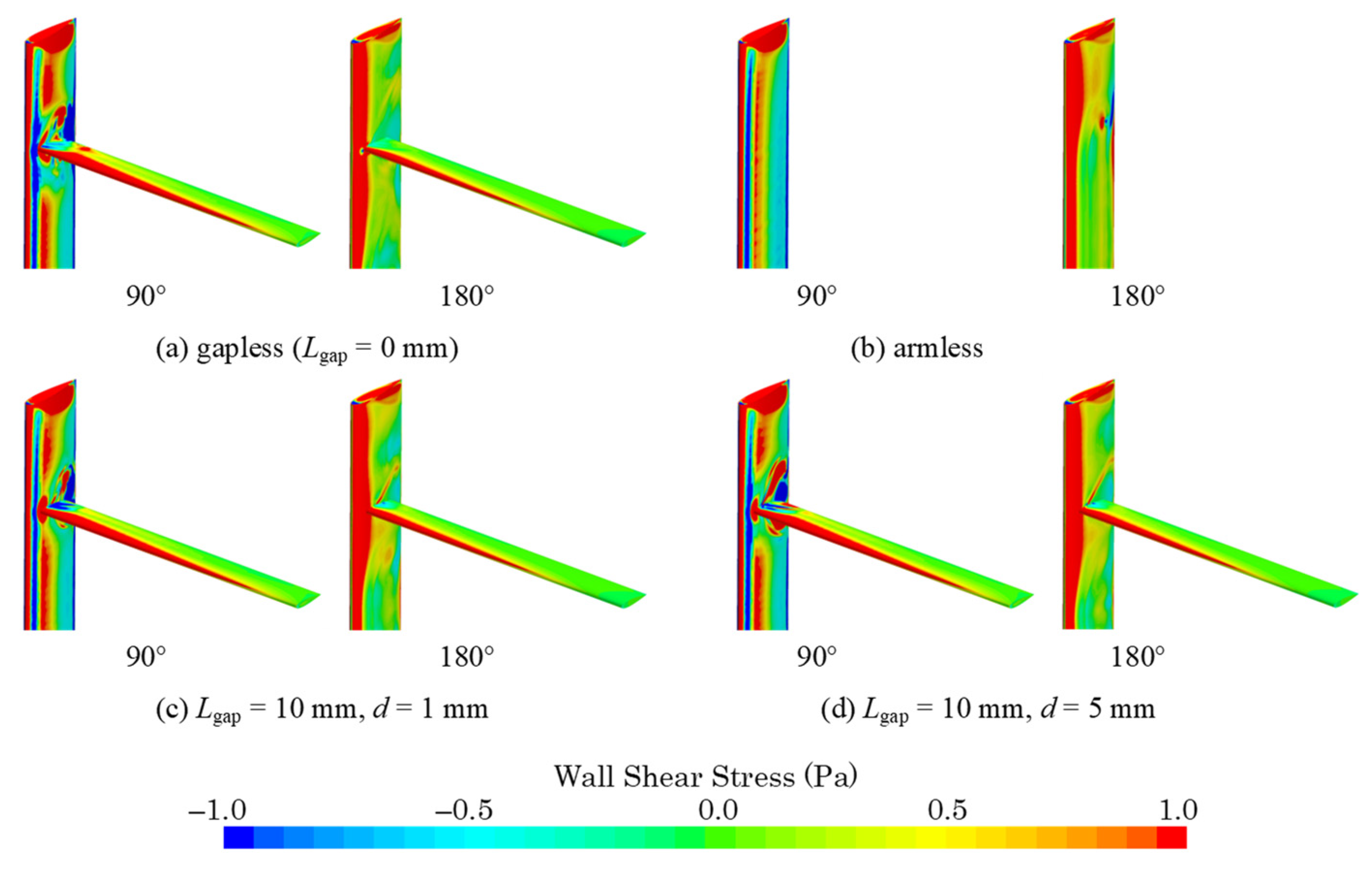
3.3. Wall Shear Stress Distribution around Connection Part

Figure 7 illustrates the wall shear stress distribution near the connection of the four–rotor models shown in Figure 6. In addition, the wall shear stress distribution of model 7 (armless) in Figure 7b is clearly different from those of the other rotors with arms. In particular, focusing on the distribution of azimuth ψ = 90°, the wall shear stress in model 7 (armless rotor) is linearly distributed along the leading edge of the main blade with positive and negative values. In the other models with arms, the linear distribution of wall shear stress along the leading edge of the blade is disturbed by the existence of the arms. In addition, in the vicinity of the arm connection portion, the area where the wall shear stress becomes negative spreads even near the trailing edge of the main blade. The degree of disturbance in the wall shear stress distribution around the connection part increases in the following order: models 1, 4, and 0.

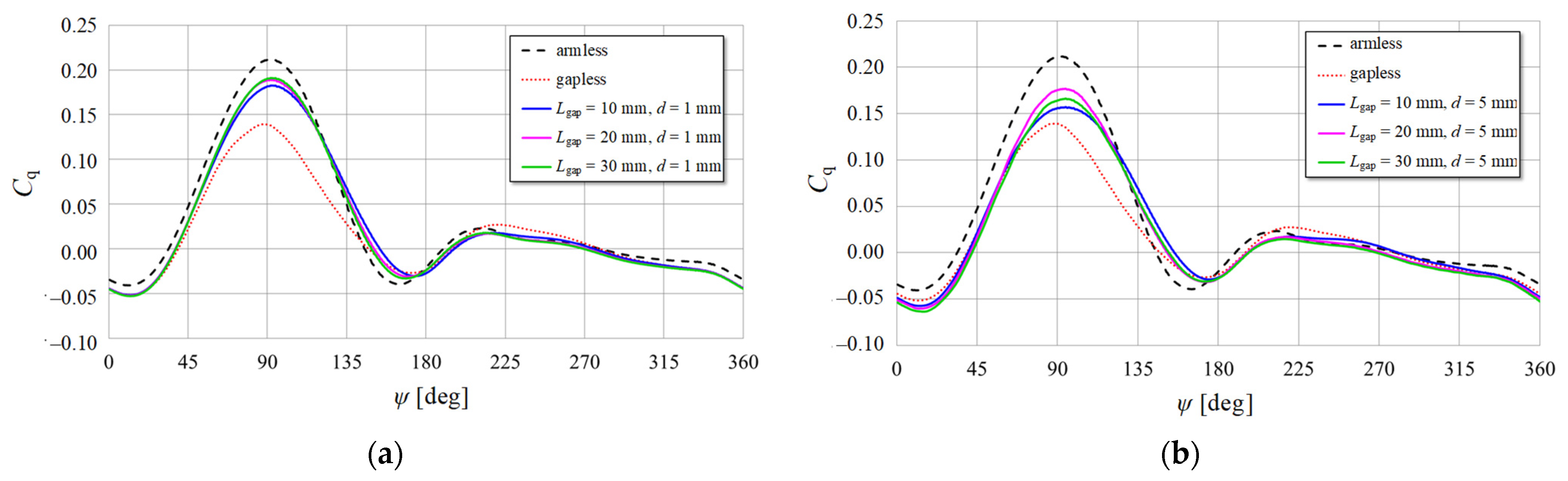
3.4. Gap Length Dependency of One-Blade Torque Variation in One Rotation

Figure 8a shows the gap–length dependence of the torque variation of one blade during one rotor rotation (seventh rotation) when the diameter of the cylindrical rod placed in the gap is d = 1 mm (models 1, 2, and 3). For comparison, the torque variations for the gapless rotor (model 0) and armless rotor (model 7) are also shown. The vertical axis in Figure 8a represents the torque coefficient C_q, which is defined by Equation (1).

$$C_{\mathrm{q}}=\frac{Q_{\mathrm{b}\mathrm{l}\mathrm{a}\mathrm{d}\mathrm{e}1}}{0.5\rho {U_{\infty }}^2\left(4H{R}^2\right)}$$

(1)

where Q_blade1 is the rotational torque of one blade, ρ is the air density (ρ = 1.225 kg/m³), and R is the rotor radius (R = D/2 = 0.375 m). Figure 8a shows that the effects of the gap length on the single–blade torque variation are small when the cylindrical rod diameter is d = 1 mm. In addition, a large difference among the models is observed around azimuth ψ = 90°. Comparing at ψ = 90°, the armless rotor (model 7) has the largest torque coefficient (C_q = 0.211), whereas the cases with d = 1 mm (models 1, 2, and 3) have approximately 10% less (C_q = 0.182, 0.189, 0.190). The gapless rotor (model 0) has the smallest value (C_q = 0.139). In the downwind half (180° < ψ < 360°), the difference in torque coefficients among the models is small.

Figure 8b depicts the variation in torque for one blade when the diameter of the cylinder is d = 5 mm (models 4, 5, and 6). The torque coefficients of the gapless and armless rotors are also shown in the figure. Similarly to Figure 8a, the difference in the torque coefficients among the models is small in the downwind half (180° < ψ < 360°). The difference among the models with d = 5 mm becomes large in the vicinity of ψ = 90°. Comparing at ψ = 90°, the C_q of models 4, 5, and 6 are 0.156, 0.175, and 0.164, respectively. There is no tendency to depend on the gap length, but all the torque coefficients at ψ = 90° of models 4, 5, and 6 decrease compared to the models of d = 1 mm. However, in the vicinity of azimuth ψ = 15°, the difference among models 4, 5, and 6 is large. In this region, the torque coefficient of model 6 (L_gap = 30 mm, d = 5 mm) is smaller than those of the other two models.

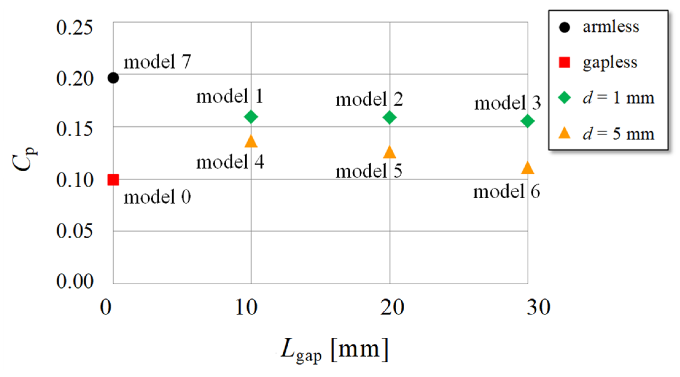
3.5. Effects of Connection Gap on Power Coefficient

Power coefficients at λ = 3 of all eight models analyzed by CFD in this study are compared in Figure 9. The horizontal axis represents the gap length L_gap, and the vertical axis represents the power coefficient C_p defined by Equation (2).

$$C_{\mathrm{p}}=\frac{P_{\mathrm{r}\mathrm{o}\mathrm{t}\mathrm{o}\mathrm{r}}}{0.5\rho {U_{\infty }}^3\left(4HR\right)}$$

(2)

In the above equation, P_rotor is the average power output obtained from the product of the angular velocity and rotational torque generated by all the blades (including the arm) during the seventh rotor revolution.

As shown in Figure 9, the C_p without arms (armless) is approximately twice that with arms (gapless), and the existence of arms significantly degrades the VAWT performance. However, the power coefficient can be improved by creating a gap between the arm and the main blade. In addition, when the diameter of the cylindrical rod placed in the gap is small (d = 1 mm), the power output is higher than that when the diameter is large (d = 5 mm). The power is improved by the gap at the connection part because the fluid passing through the gap decreases the surface pressure on the inner surface of the blade (suction side), resulting in an increase in the lift force when the blade moves near the upstream azimuth (ψ = 90°). To support this conjecture, Figure 10 shows the blade surface pressure distribution in the cross section at z = 140 mm (15 mm above the arm neutral line) when blade 1 is at ψ = 90°. Figure 10 separately compares the pressure coefficients of model 0 without a gap, model 1 with a gap, and model 7 without arms (as a reference) for the outer surface (pressure side: broken line) and the inner surface (suction side: solid line). The pressure coefficient C_pre in Figure 10 is defined by Equation (3):

$$C_{pre}=\frac{∆p}{0.5\rho {\left(R\omega \right)}^2}$$

(3)

where Δp is the surface pressure (gauge pressure) of the blade.

As shown in Figure 10, there is no significant difference in the pressure distributions of the outer blade surface among the models. As a reference, Figure A2 and Figure A3 in the Appendix A show the distribution of the surface pressure and wall shear stress on the outer surface of the blade; almost no difference is observed between the presence and absence of gaps. However, the pressure distributions on the inner surface of the blade differed considerably among the models, as shown in Figure 10. The area enclosed by the pressure coefficient curves on the outer and inner sides of the blade corresponds to the lift force. If the area of the armless model is assumed to be 100%, then those of models 1 and 2 are 87% and 43%, respectively. The figure shows that the provision of a gap improves the lift generated by the blade near the connection portion compared with the case without the gap.

As shown in Figure 9, the power coefficient decreases as the gap length increases, regardless of the diameter of the cylindrical rod installed in the gap. This can be explained by the replacement of the airfoil cross section with a small drag coefficient (2D–C_d = approximately 0.02 [19] at Re_arm = 5.5 × 10⁴) with the cylindrical cross section with a large drag coefficient (2D–C_d = approximately 1.2 [20]). To give a concrete example in the present numerical analysis, the surface pressure distribution in the cross section at the local radius r = 0.36 m (mid–gap) of the connecting rod (d = 5 mm) of model 6 is shown in Figure 11, compared with that of model 0 (airfoil arm) without gaps, when the arm 1 is at ψ = 0°. The pressure coefficient shown in Figure 11 is defined by Equation (4).

$$C_{pre}=\frac{∆p}{0.5\rho {\left(U_{\infty }+r\omega \right)}^2}$$

(4)

From the pressure distribution shown in Figure 11, the drag forces per unit length are calculated to be 0.55 N/m and 1.64 N/m for the airfoil arm (model 0) and cylindrical rod, respectively. The drag force of the connecting rod is approximately three times that of the arm. However, the effect of wall friction is neglected because it is relatively small (see [14]). In this case, the calculated drag coefficients of the airfoil arm and cylindrical rod are C_d = 0.17 and C_d = 0.73, respectively, which are somewhat different from the abovementioned two–dimensional values (2D–C_d) due to 3D effects.

The above results imply that it is desirable to create a short gap between the arm and the main blade of VAWT within the permissible range of structural strength to improve the power output. In addition, it is necessary to minimize the cross–sectional area of the connecting member in the gap. Figure 12 shows the schematic of the blade–arm connection part using a cylindrical rod of d = 5 mm when the L_gap is gradually shortened from 10 mm to 5 mm. Numerical analysis for cases with less than L_gap = 10 mm were not conducted in this study because the generation of reasonable mesh becomes difficult as the gap becomes shorter. As shown in Figure 12, when L_gap = 7.2 mm, the arm end surface touches the main blade surface, and as L_gap becomes even shorter, the cross–sectional area of the blade–arm connection increases. In this case, C_p shown in Figure 9 can be inferred to approach the value of C_p in model 0 from that in model 4. Ideally, when applied to an actual VAWT, connecting the arm and main blade with a member whose thickness does not exceed the arm thickness (7.2 mm in this model) within the range of L_gap = 7.5 to 10 mm (L_gap/R = 0.0200 to 0.0267) is recommended.

4. Conclusions

To investigate the effects of a gap that was placed between the blade and the arm of a vertical–axis wind turbine (VAWT), a computational fluid dynamics analysis was conducted for eight models of a two–bladed H–type VAWT (diameter: 0.75 m, height: 0.5 m) as the object, including the gap–length conditions of L_gap/R = 0.0267, 0.0533, and 0.0800. The visualization of vortex shedding using the Q–criterion isosurfaces showed that the size of the vortices generated from the connection portion was smaller with a gap than without. The surface pressure and wall shear stress distributions approached those of the armless rotor owing to the gap. Regarding the azimuth dependence of the single–blade torque, a significant difference in the effect of the gap was observed in the upstream range (near azimuth ψ = 90°). When assuming the power of the armless rotor at the tip speed ratio λ = 3 as 100%, those of the gapless rotor and the rotor, which had a connection rod (d = 10 mm, d/c = 0.125) in the shortest gap, became approximately 50% and 81%, respectively. However, the power coefficient decreased as the gap length increased. Moreover, the power coefficient decreased further as the diameter of the cylindrical rod placed in the gap increased. It is well known that applying an airfoil shape to the cross section of an arm effectively reduces the aerodynamic resistance of VAWTs when it is necessary to install the arm. Thus, providing a gap at the blade–arm connection part and reducing the cross–sectional area of the connecting member are effective in reducing the output loss caused by the connection portion.

References

1. Ahmed, N.A.; Cameron, M. The challenges and possible solutions of horizontal axis wind turbines as a clean energy solution for the future. Renew. Sustain. Energy Rev. 2014, 38, 439–460. [Google Scholar] [CrossRef]
2. Luo, L.; Zhang, X.; Song, D.; Tang, W.; Yang, J.; Li, L.; Tian, X.; Wen, W. Optimal design of rated wind speed and rotor radius to minimizing the cost of energy for offshore wind turbines. Energies 2018, 11, 2728. [Google Scholar] [CrossRef]
3. Islam, M.; Fartaj, A.; Carriveau, R. Analysis of the design parameters related to a fixed-pitch straight-bladed vertical axis wind turbine. Wind Eng. 2008, 32, 491–507. [Google Scholar] [CrossRef]
4. Islam, M.; Ting, D.S.K.; Fartaj, A. Aerodynamic models for Darrieus-type straight-bladed vertical axis wind turbines. Renew. Sustain. Energy Rev. 2008, 12, 1087–1109. [Google Scholar] [CrossRef]
5. Kumar, R.; Raahemifar, K.; Fung, A.S. A critical review of vertical axis wind turbines for urban applications. Renew. Sust. Energ. Rev. 2018, 89, 281–291. [Google Scholar] [CrossRef]
6. Li, Y.; Calisal, S.M. Three-dimensional effects and arm effects on modeling a vertical axis tidal current turbine. Renew. Sustain. Energy Rev. 2010, 35, 2325–2334. [Google Scholar] [CrossRef]
7. Qin, N.; Howell, R.; Durrani, N.; Hamada, K.; Smith, T. Unsteady flow simulation and dynamic stall behaviour of vertical axis wind turbine blades. Wind Eng. 2011, 35, 511–527. [Google Scholar] [CrossRef]
8. De Marco, A.; Coiro, D.P.; Cucco, D.; Nicolosi, F. A numerical study on a vertical-axis wind turbine with inclined arms. Int. J. Aerosp. Eng. 2014, 2014, 180498. [Google Scholar] [CrossRef]
9. Marsh, P.; Ranmuthugala, D.; Penesis, I.; Thomas, G. Three-dimensional numerical simulations of straight-bladed vertical axis tidal turbines investigating power output, torque ripple and mounting forces. Renew. Energy 2015, 83, 67–77. [Google Scholar] [CrossRef]
10. Li, Q.A.; Maeda, T.; Kamada, Y.; Murata, J.; Shimizu, K.; Ogasawara, T.; Nakai, A.; Kasuya, T. Effect of solidity on aerodynamic forces around straight-bladed vertical axis wind turbine by wind tunnel experiments (depending on number of blades). Renew. Energy 2016, 96, 928–939. [Google Scholar] [CrossRef]
11. Aihara, A.; Mendoza, V.; Goude, A.; Bernhoff, H. A numerical study of strut and tower influence on the performance of vertical axis wind turbines using computational fluid dynamics simulation. Wind Energy 2022, 25, 897–913. [Google Scholar] [CrossRef]
12. Kirke, B.K.; Lazauskas, L. Limitations of fixed pitch Darrieus hydrokinetic turbines and the challenge of variable pitch. Renew. Energy 2011, 36, 893–897. [Google Scholar] [CrossRef]
13. The SeaTwirl Concept. Web Page. Available online: https://seatwirl.com/products/ (accessed on 19 September 2023).
14. Hara, Y.; Horita, N.; Yoshida, S.; Akimoto, H.; Sumi, T. Numerical analysis of effects of arms with different cross-sections on straight-bladed vertical axis wind turbine. Energies 2019, 12, 2106. [Google Scholar] [CrossRef]
15. Mertens, S.; van Kuik, G.; van Bussel, G. Performance of an H-Darrieus in the skewed flow on a roof. J. Sol. Energy Eng. 2003, 125, 433–440. [Google Scholar] [CrossRef]
16. Menter, F.R. Two-equation eddy-viscosity turbulence models for engineering applications. AIAA J. 1994, 32, 1598–1605. [Google Scholar] [CrossRef]
17. Van Bussel, G.J.W.; Polinder, H.; Sidler, H.F.A. TURBY®: Concept and realisation of a small VAWT for the built environment. In Proceedings of the EAWE/EWEA Special Topic Conference “The Science of Making Torque from Wind”, Delft, The Netherlands, 19–21 April 2004; p. 8. [Google Scholar]
18. Fu, W.-S.; Lai, Y.-C.; Li, C.-G. Estimation of turbulent natural convection in horizontal parallel plates by the Q criterion. Int. Commun. Heat Mass Transf. 2013, 45, 41–46. [Google Scholar] [CrossRef]
19. Sheldahl, R.E.; Klimas, P.C. Aerodynamic Characteristics of Seven Symmetrical Airfoil Sections through 180-Degree Angle of Attack for Use in Aerodynamic Analysis of Vertical Axis Wind Turbines; SAND-80-2114; Sandia National Labs.: Albuquerque, NM, USA, 1981; pp. 43–44. [Google Scholar]
20. White, F.M. Fluid Mechanics, 4th ed.; McGraw-Hill: New York, NY, USA, 1999. [Google Scholar]
Figure 1. Rotor model: (a) perspective view; (b) top view.
Energies 16 06925 g001
Figure 2. Computational domain of the present CFD.
Energies 16 06925 g002
Figure 3. Computational mesh around the wind turbine rotor.
Energies 16 06925 g003
Figure 4. Details of the computational mesh around the wind turbine rotor and the definition of a gap at the connection portion: (a) rotation and wake regions (static region 2); (b) near–blade and near–arm regions; (c) mesh around a blade and a blade–arm connection gap.
Energies 16 06925 g004
Figure 5. Azimuth dependency of vortex shedding (Q–criterion isosurfaces: Q = 1000 s−2) and vorticity in the cases of (a) gapless and (b) 10 mm gap with d = 1 mm.
Energies 16 06925 g005
Figure 6. Surface pressure distribution in the cases of (a) gapless, (b) armless, (c) 10 mm gap with d = 1 mm, and (d) 10 mm gap with d = 5 mm.
Energies 16 06925 g006
Figure 7. Wall shear stress distribution in the cases of (a) gapless, (b) armless, (c) 10 mm gap with d = 1 mm, and (d) 10 mm gap with d = 5 mm.
Energies 16 06925 g007
Figure 8. Variation in the torque coefficient of a blade: (a) d = 1 mm; (b) d = 5 mm.
Energies 16 06925 g008
Figure 9. Dependence of power coefficient on gap length.
Energies 16 06925 g009
Figure 10. Pressure coefficient distribution on a blade at z = 140 mm when ψ = 90°.
Energies 16 06925 g010
Figure 11. Pressure coefficient distribution on an arm or a cylindrical rod at r = 360 mm when ψ = 0°.
Energies 16 06925 g011
Figure 12. Schematic of the blade–arm connection part when d = 5 mm: (a) Lgap = 10 mm; (b) Lgap = 7.5 mm; (c) Lgap = 7.2 mm; (d) Lgap = 7.0 mm; (e) Lgap = 6.8 mm; (f) Lgap = 6.5 mm; (g) Lgap = 6.0 mm; (h) Lgap = 5.0 mm.
Energies 16 06925 g012